The final version of this paper has been published in Biological Conservation, 2009, 142, 779-788, doi:10.1016/j.biocon.2008.12.014
Smart spatial incentives for market-based conservation

Abstract

Market-based instruments such as payments, auctions or tradable permits have been proposed as flexible and cost-effective instruments for biodiversity conservation on private lands. Trading the service of conservation requires one to define a metric that determines the extent to which a conserved site adds to the regional conservation objective. Yet, while markets for conservation are widely discussed and increasingly applied, little research has been conducted on explicitly accounting for spatial ecological processes in the trading. In this paper, we use a coupled ecological-economic simulation model to examine how spatial connectivity may be considered in the financial incentives created by a market-based conservation scheme. Land use decisions, driven by changing conservation costs and the conservation market, are simulated by an agent-based model of land users. On top of that, a metapopulation model evaluates the conservational success of the market. We find that optimal spatial incentives for agents correlate with species characteristics such as the dispersal distance, but they also depend on the spatio-temporal distribution of conservation costs. We conclude that a combined analysis of ecological and socio-economic conditions should be applied when designing market instruments to protect biodiversity.

1 Introduction

Market-based instruments such as payments (Wunder, 2007; Drechsler et al., 2007), auctions (Latacz-Lohmann and Van der Hamsvoort, 1998) or biodiversity offset trading (Panayotou, 1994; Chomitz, 2004) have been suggested as a means to complement existing reserves by inducing biodiversity protection on private lands. Market-based instruments are currently being used or tested in many countries around the world. Some examples are conservation and wetland mitigation banking in the US (Salzman and Ruhl, 2000; Wilcove and Lee, 2004; Fox and Nino-Murcia, 2005) or markets schemes in Australia (Coggan and Whitten, 2005; Latacz-Lohmann and Schilizzi, 2005). One of the reasons for the increasing popularity of these instruments is the realization that markets may achieve a more targeted and therefore more cost-efficient correction of a conservation problem, in particular because landowners have more information about their local costs and can choose the allocation of conservation measures accordingly (Jack et al., 2008). Another reason is that market-based instruments are well suited for targeting multiple ecosystem services (e.g. conservation and carbon sequestration (Nelson et al., 2008)), a point which has been highlighted in a recent statement of the European Union (EU-Commission, 2007).

At the same time, however, there has been considerable concern over whether current implementations of conservation markets target the right entities. At present, market-based policies for conservation tend to use simple and indirect incentives, such as payments for certain farming practices (Ferraro and Kiss, 2002). But are those incentives efficient in protecting threatened species, or are we paying "money for nothing" (Ferraro and Pattanayak, 2006)? Examining the structure of the given incentives for landowners is the key to answering these questions. What defines a unit of conservation? What are we paying landowners for?

The overall goal of global conservation efforts is to ensure the persistence of biodiversity in our landscapes (Margules and Pressey, 2000). Therefore, it would be ideal to assess the market value of a conservation measure directly by assessing its effect on species survival (Williams and Araujo, 2000; Bruggeman and Jones, 2008). Unfortunately, applying this method to real-world situations is often not feasible because direct monitoring or detailed population models are too expensive or not available (Jack et al., 2008). Moreover, the efficiency of markets crucially depends on the information available to landowners. If landowners do not understand the evaluation criteria for their land, they may choose suboptimal land configurations, or they may decide not to participate in the market at all. Therefore, practically all existing market schemes use a metric, given by a number of indices, that relates measurable quantities of a site (e.g. size) to the site’s market value.

Most of these existing schemes (e.g. habitat banking in the US) base their evaluation solely on the quality and size of the local site without considering its surroundings. This raises some concern because in many cases, the ecological value of a typical private property (e.g. arable field, forest lot) does in fact depend on neighboring properties. Populations or ecosystems may exhibit thresholds for the effectiveness of conservation measures, which implies that a local measure may be ineffective when it is not accompanied by other measures. (Hanski et al., 1996; Scheffer et al., 2001). Furthermore, for many endangered species, not only the absolute loss of habitat area, but also habitat fragmentation is a major cause of population decline (compare e.g. Saunders et al., 1991; Fahrig, 2002). Therefore, metrics that only evaluate sites locally may set the wrong incentives because they do not correspond to the real conservational value of a site.

Spatial metrics that consider the surrounding of a site are available and are widely used for systematic reserve site selection (e.g. Moilanen, 2005; van Teeffelen et al., 2006). Yet, simply transferring spatial metrics from conservation planning into connectivity dependent incentives for landowners (in the following we will call such incentives short "spatial incentives") would be short sighted. Conservation planning metrics have been developed for assessing and optimizing the ecological value of a habitat network from the viewpoint of a planner who considers the whole landscape. Landowners in conservation markets, on the other hand, react to the given incentives independently and with limited knowledge, striving for maximization of their individual utility rather than maximizing global welfare. The fact that the value of a site depends on neighboring sites implies that land use decisions may create costs or benefits for neighboring landowners. In economics, such costs or benefits are referred to as externalities. It is well known that markets may fail to deliver an optimal allocation of land use in the presence of such externalities (Mills, 1980). Another problem is that, unless we assume perfect information and unlimited intellectual capacities, we must take into account that landowners may fail to find the optimal adoption of their land use in the presence of complicated spatial evaluation rules (Hartig and Drechsler, submitted). Thus, the need to consider human behavior in metrics for market-based instruments is characterized by a trade-off: Ecological accuracy calls for a metric that is complex enough to capture all details of the relevant ecological processes, but socio-economic reality may suggest compromises towards more practical and robust metrics.

In this paper, we combine a spatially explicit population model with an agent-based simulation model to assess the effect of connectivity-dependent incentives in a virtual conservation market. One key assumption is that landowners do not react optimally to the given incentives, but base their decisions only on the present land configuration and their estimated costs and benefits for the next period. Thus, we seek to optimize for ecological parameters such as dispersal as well as for economic parameters such as behavior of landowners. To simulate the reactions of landowners towards a given spatial metric, we use the conservation market model introduced in (Hartig and Drechsler, submitted). A spatially explicit metapopulation model is placed on top of the emerging landscape structure to evaluate the conservation success for different species in terms of survival probability at a fixed time horizon.

2 Methods

2.1 Overview and purpose

The aim of this study is to design spatial incentives that result in cost-effective conservation when there are many landowners and the conservation outcome depends on the combination of decisions by landowners. Here, cost-effective means that we maximize the conservation effect at a given budget. The model used contains two submodels: An economic submodel that simulates the trading of conservation credits and an ecological submodel to assess the viability of several species in the dynamic landscape that emerges from the trading activity. The driver for trading and the subsequent change of the landscape configuration is economic change in the region, reflected by heterogeneously changing costs of maintaining a local site in a conserved state. We first describe the state variables of the model, followed by the economic and the ecological submodel and the coupling of the submodels. The coupled model is then used to find the cost-effective metric by comparing the forecasted species persistence across a range of different parameterizations of the metric. Fig. 1 shows a graphical representation of our model approach.

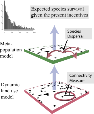
Figure 1: Modelling approach: Drivers are spatially heterogeneous, dynamic costs for each site. On the basis of these costs and the spatial incentives, conservation measures are allocated by the economic submodel. The resulting dynamic landscape is used as an input for the ecological model, which estimates species survival probabilities on this landscape.

2.2 State variables and scales

The simulation is conducted on a rectangular $30\times 30$ grid with periodic boundary conditions (i.e. the grid has the topology of a torus). The $n=30^{2}$ grid cells represent both the economic (property) units and the ecological (habitat) units. Although the model may be applied to any spatial and temporal scale, we think of grid cells as being of the size of an average agricultural field in Europe (around $10$ ha), and time steps being a year. Grid cells $x_{i}$ occur in two states: They can be conserved at a cost $c_{i}$ and thus provide habitat for the species, or they are used for other economic purposes, resulting in no costs. The conservation state of a grid cell is labelled with $\sigma_{i}$, $\sigma_{i}=1$ being a conserved cell and $\sigma_{i}=0$ being an unconserved cell. Conserved grid cells may be either occupied (populated) $p_{i}=1$ or unoccupied $p_{i}=0$ by the species under consideration. Unconserved grid cells can never be occupied. A list of the state variables and parameters of the two submodels is given in Table 1.

Symbol	Connotation	Range
State variables:
$x_{i}$	Position of the i-th cell on the grid
$\sigma_{i}(t)$	Conservation state of the i-th cell	$\{0,1\}$
$p_{i}(t)$	Population state of the i-th cell	$\{0,1\}$
$c_{i}(t)$	Opportunity costs of $\sigma_{i}$ = 1 at t	around $1$
Parameters economic model:
$\Delta$	Cost heterogeneity	$[0..1]$
$\omega$	Cost correlation	$[0..\infty]$
$m$	Connectivity weight	$[0..1]$
$l$	Connectivity length	$[0..\infty]$
$\lambda$	Budget constraint	$[0..\infty]$
Parameters ecological model:
$e$	Local extinction risk	$[0..1]$
$r$	Emigration rate	$[0..\infty]$
$r_{d}$	Emigration rate after destruction	$[0..\infty]$
$\alpha^{-1}$	Dispersal distance	$[0..\infty]$

Table 1: List of state variables (top), parameters of the economic model (middle) and parameters of the ecological model (bottom). Note that although we omit to denote the time dependence $(t)$ explicitly throughout the main text, all state variables and expressions derived from state variables are time dependent.

2.3 Economic model

The economic model describes the decisions of landowners to establish, maintain, or quit a conservation measure on their land (grid cell) in each period. Landowners decisions are based on whether conservation or alternative land use generates a higher return. The returns on the two land use types are influenced by dynamic, spatially heterogeneous costs for conserving a grid cell and by the metric of the conservation market, which decides on the amount of conservation credits to be earned with a particular site, and by the current market price for conservation credits. The model is designed as a spatially explicit, agent-based partial equilibrium model (compare Drechsler and Wätzold, in press; Hartig and Drechsler, submitted).

A conserved grid cell $x_{i}$ produces a certain amount of conservation credits $\xi_{i}$ depending on the number of conserved grid cells in its neighborhood. We use the following metric to determine $\xi_{i}$:

$$\xi_{i}=(1-m)+m\cdot\zeta_{i}(l)\;.$$ (1)

The first term $1-m$ is independent of the connectivity and may be seen as a base reward for the conserved area. The parameter $m$ is a weighting factor that determines the importance of connectivity compared to area. The second term $m\cdot\zeta(l)$ includes the connectivity of the site, measured by the proportion of conserved sites within a circle of radius $l$:

$$\zeta_{i}(l)=\left(\sum_{d_{ij}<l}\sigma_{j}\right)\cdot\left(\sum_{d_{ij}<l}1\right)^{-1}\;.$$ (2)

Here, $d_{ij}$ refers to the distance between the focal cell $x_{i}$ and another cell $x_{j}$. Fig. 2 shows a graphical illustration of this connectivity measure. The total amount of credits in the market is given by the sum of $\xi_{i}$ over all conserved grid cells:

$$U=\sum_{i=1}^{n}\sigma_{i}\xi_{i}\;.$$ (3)

The conservation of a site results in costs that differ among grid cells. Conservation costs may vary over space and time (Ando et al., 1998; Polasky et al., 2008). We use three different algorithms to generate pattern of random dynamic costs $c_{i}(t)$. All algorithms create average costs of 1, but they differ in the spatial and temporal distribution of costs. Algorithm 1 generates spatially and temporally uncorrelated random costs by drawing from a uniform distribution of width $2\Delta$ at each time step. Algorithm 2 creates spatially uncorrelated, but temporally correlated costs by applying on each grid cell a random walk of maximum step length $\Delta$ together with a small rebounding effect that pushes costs towards $1$ with strength $\omega$. Algorithm 3 creates spatio-temporally correlated costs, using a random walk of maximum step length $\Delta$ combined with a spatial correlation term that pushes costs with strength $\omega$ towards the average costs in the neighborhood. A mathematical description of the three algorithms is given in appendix A, together with figures of the created cost distributions (Fig. 7 and Fig. 8).

To simulate trading, we introduced a market price $P$ for credits. The benefits to be earned by a site are given by $P\cdot\xi$ where $\xi$ is the amount of credits to be earned by a site (eq. 1). Based on his costs and the potential benefits, each landowner decides whether to conserve his land or not. The model has two options for determining the equilibrium price of the market: Either the price is adjusted until a certain target level for the total amount of produced conservation credits $U$ (eq. 3) is met, or the price is adjusted until a certain level of aggregated costs for the conservation is reached. By aggregated costs, we mean the sum of the costs of all conserved sites:

$$C=\sum_{i=1}^{n}\sigma_{i}c_{i}\;.$$ (4)

Fixing the target reflects a situation where the quantity of conservation credits is fixed. This is, for example, the case in a tradable permit scheme. Fixing the costs, on the other hand, could correspond to a payment scheme where a conservation agency buys credits until a budget constraint is reached. The two options differ when global properties of the cost distribution, such as the mean, change over time. In our simulation, however, costs are in a steady state that is normalized to a mean of $1$. Thus, both options are approximately identical except for finite size effects, which would disappear in the limit of an infinitely large landscape. We chose the second option of fixing the budget for the analysis because it allows an easier comparison between different metrics. Appendix B.1 gives a detailed description of the scheduling of the economic model.

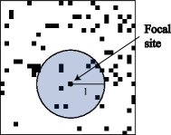
Figure 2: Illustration of the connectivity measure: The connectivity $\zeta_{i}(l)$ is the fraction of conserved sites within a circle of radius $l$ of the focal site

2.4 Ecological model

To evaluate conservation success in the emerging dynamic landscapes, we use a stochastic metapopulation model (Hanski, 1998, 1999). Each conserved grid cell is treated as a habitat patch, meaning that each grid cell may hold a local population of the species. Local populations produce emigrants which may disperse and establish a new local population on an unoccupied cell. At the same time, local populations are subject to local extinction, which may be caused e.g. by demographic or environmental stochasticity. The population as a whole can persist on the landscape if the average recolonization rate is higher than the average local extinction risk, yet, stochastic fluctuations of the number of occupied patches may eventually cause extinction of the whole metapopulation. The better the connectivity among patches, and the more patches in the network, the lower the probability of such a global extinction.

Local extinctions are modelled by a constant chance $e$ of each local population to go extinct per time step. The amount of dispersers arriving from a source patch $x_{j}$ at a target patch $x_{i}$ is given by the following dispersal kernel:

$$p_{ij}=r\cdot\frac{1}{\sum_{i}\sigma_{i}-1}\cdot e^{-\alpha\cdot d_{ij}}\;,$$ (5)

where $r$ is the emigration rate, the term $(\sum_{i}\sigma_{i}-1)^{-1}$ divides the number of dispersing individuals by the available habitat patches, and the exponential term describes mortality risk during dispersal as a function of distance between $x_{i}$ and $x_{j}$. If a patch has been destroyed at the current time step, we set the emigration rate to $r_{d}$, assuming that a proportion of $r_{d}$ of the population will be able to disperse before destruction. The sum of all arriving immigrants according to eq. 5 (truncated to 1) is taken as the probability that this patch is colonized at the current time step. Appendix B.2 gives a detailed description of the scheduling of the ecological model.

2.5 Parametrization and analysis of the model

Different species have different connectivity requirements depending on their dispersal abilities. Therefore, we expect an optimized spatial metric to reflect this by values of the connectivity weight $m$ and the connectivity length $l$ that are related to the species characteristics $r,r_{d}$ and $\alpha$. Additionally, optimal values for $m$ and $l$ may be affected by economic conditions, i.e. the distribution of conservation costs. To analyze the effect of species characteristics and the cost distribution on the optimal spatial incentive, we varied both the connectivity weight $m$ and the connectivity length $l$ of the metric eq. 1 for three different cost scenarios and for three different species types.

The three cost scenarios were generated by Algorithm 1 at $\Delta=0.2$, Algorithm 2 at $\Delta=5\cdot 10^{-5}$ and $\omega=0.0065$, and Algorithm 3 at $\Delta=0.015$ and $\omega=0.006$. Table 2 displays a summary of the three scenarios. Remember that the first scenario creates uncorrelated costs, the second creates temporally correlated costs and the third scenario creates spatio-temporally correlated costs. Figs. 7 and 8 in Appendix A show the spatial and temporal cost distribution generated by the chosen parameters.

Cost Scenario	Parameters	Characteristics
1 - Random	$\Delta=0.2$	uncorrelated
2 - Random walk	$\Delta=5\cdot 10^{-5}$	time correlated
	$\omega=0.0065$
3 - Correlated walk	$\Delta=0.015$	space and time
	$\omega=0.006$	correlated

Table 2: Overview of the cost scenarios created by the three algorithms.

For the species, we consider three functional types: Short-range, intermediate and global dispersers. The parametrization for the three species is displayed in Table 3. To assess the extinction risk for the species, we ran the simulation with different random economic starting conditions between 300 and 1000 times and calculated the probability of a metapopulation extinction after 1000 time steps.

Species type	$\mathbf{e}$	$\mathbf{r}$	$\mathbf{r_{d}}$	$\mathbf{\alpha^{-1}}$
I - short dispersal	0.29	3	1	5
II - intermediate dispersal	0.51	3	1	25
III - global dispersal	0.66	3	1	1000

Table 3: Parameter values for the three species types considered. $\mathbf{\alpha^{-1}}$ is the typical dispersal distance, measured in units of the grid cell length. With cell lengths of $100$ m, this translates to typical dispersal distances of 0.5 km, 2.5km and 100 km, respectively.

The budget constraint $\lambda$ for the aggregated costs (eq. 4) was fixed at 0.03 times the number of grid cells $n$ for scenarios with cost dynamics generated by the random walk algorithms (economic scenarios 2 and 3) and at 0.05 times the number of grid cells $n$ for the scenarios created with the random algorithm (economic scenario 1). Exceptions are the combination economic scenario 3 with species 3, where aggregated costs were set at 0.1 times $n$ and economic scenario 1 with species 3, where aggregated costs were set at 0.18 times $n$. The adjustment to different budgets was done to create similar survival probabilities across the nine scenarios formed by systematic combination of the three cost scenarios and the three species types.

Figure 3: Effect of the connectivity weight $m$ and the connectivity length $l$. The pictures show typical landscape structures emerging from trading with costs being sampled by Algorithm 2 at $\Delta=5\cdot 10^{-5},\omega=0.0065$. Conserved sites are colored black, other sites are colored white. The top row is created with a long connectivity length ($l=10$), the bottom row with a short connectivity length ($l=1.5$). The pictures in the left column are taken at $m=0$, which means that no weight is put on connectivity. Consequently, the landscape structure is dominated by the sites of lowest costs. Increasing connectivity weight ($m=0.5$ middle, $m=1$ right) results in increasing clustering of conserved sites, but in a smaller total area. At a connectivity weight of $m=1$, meaning that all weight is put on connectivity, $l=1.5$ results in a very dense cluster, while the larger connectivity length $l=10$ results in a more spread out configuration.

3 Results

3.1 Emerging landscapes

For all cost scenarios and all connectivity lengths, an increase in connectivity weight results in more aggregated landscape structures. The density of the clustering is controlled by the connectivity length $l$, which determines how close patches have to be to be counted as connected. Smaller connectivity lengths ($l\sim 1.5$, corresponding to the direct 8-cell neighborhood) result in very dense clusters at full connectivity weight, while larger connectivity lengths lead to more loose agglomerations of conserved sites. Due to the spatial cost heterogeneity, there is a trade-off between clustering and area: At a fixed budget, a higher connectivity weight results in lower total area, but with higher clustering. Typical landscapes are displayed in Fig. 3.

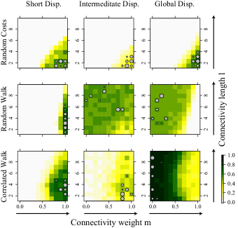
Figure 4: Survival probability as a function of connectivity weight (x-axis) and connectivity length (y-axis) for the three species types (columns 1-3) and for three cost scenarios (rows 1-3). Dark values represent high survival probabilities. The gray circles mark the seven combinations of $m,l$ that yielded the highest survival probabilities, with larger circle size indicating a better ranking within these seven combinations. For most of the scenarios, these optimal points cluster in one small area of the parameter range. The uncertainty of the survival probability can be estimated from a binomial error model. Typical values of the absolute standard error are in the order of $0.01$. This explains why there is some remaining spread of the best combinations of $m,l$ when $m\simeq 0$ is favored (meaning that $l$ has little influence on the model) or when survival probabilities are very similar within a larger area of ($m,l$).

3.2 Optimal incentive

To find the most effective spatial metric ($m,l$), we varied connectivity weight between 0 and 1 and connectivity length between 1.5 and 9.5 in 11 linear steps. Note that a conservation market with no spatial trading rules corresponds to a value of $m=0$. The resulting survival probabilities after 1000 years for the three cost scenarios and the three species types are shown in Fig. 4. The results show that a short disperser such as species I may gain substantially from a very high connectivity weight and short to medium connectivity lengths, while globally dispersing species such as species III benefit from a low connectivity weight and are relatively insensitive towards the connectivity length. For intermediate species such as species II, the tendency changes depending on the cost scenario. An exception is the cost scenario 1 with random costs, which requires very high connectivity weight and short connectivity lengths for all species. We will discuss the reasons for this in the next subsection.

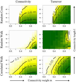
Figure 5: Resulting mean connectivity and turnover for the three cost scenarios as a function of connectivity weight $m$ and connectivity length $l$. Connectivity is measured as the mean of $\zeta(1.5)$ of all conserved sites. Turnover, the fraction of conserved sites that are destroyed and recreated elsewhere per time step, serves as an estimate for the intensity of landscape dynamics. Dark values represent low turnover and high connectivity, respectively.

3.3 Interpretation of the results

The observed influence of the cost scenarios on the effectiveness of the applied metric ($m,l$) suggests that the emerging landscapes differ among the different cost scenarios. To analyze this difference, we plotted landscape connectivity as well as turnover (the fraction of conserved sites that are destroyed and recreated elsewhere per time step) as a function of the metric parameters $m$ and $l$ for the three considered cost scenarios (Fig. 5).

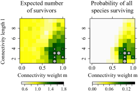
Figure 6: Expected number of surviving species (right) and probabilities of all species surviving (left) for the spatio-temporally correlated costs of scenario 3. The gray circles mark the seven combinations of $m,l$ which yielded the highest score of the applied measure, with larger circle size indicating a better ranking within these seven combinations.

The results show that greater temporal randomness in the costs causes higher turnover, in that landowners switch rapidly between conserving and not conserving. This increase in turnover effectively increases the local extinction risk, because local populations go extinct at the destroyed sites, while the remaining subpopulations can not immediately recolonize the new sites. Creating connected patches leads to more stability, as neighborhood benefits may outweigh the individual variation in cost for a cell. Thus we are not only facing a trade-off between area and connectivity, but a trade-off between area, connectivity and turnover. The latter explains why different economic scenarios lead to different optimal metrics: For random costs as in scenario 1, turnover rates are very sensitive to the chosen spatial metric. Consequently, turnover totally dominates species survival and high connectivity weight is favored for all species because it reduces the turnover rate. In contrast, the spatial metric hardly affects turnover for scenario 2 and scenario 3. Here, the optimization results (Fig. 4) only reflect the trade-off between connectivity and area: Short range dispersers require high connectivity weights, while global dispersers prefer larger areas.

3.4 Multiple-species optimization

Assuming that all three species defined in Table 3 share the same habitat, but do not interact, we can also use our model to generate recommendations on how to support all three species at the same time. There are several options available to combine the survival of multiple species into one index (Nicholson and Possingham, 2006; Hartig and Drechsler, 2008). Here, we use two common indices. The first is the expected number of surviving species, which is given by the sum of the survival probabilities of all species. The second index is the probability of all species surviving, given by the product of the survival probabilities of all species. As for the single species case, both indices were calculated for a time horizon of 1000 years. Fig. 6 shows the resulting scores for the spatio-temporally correlated cost scenario. Both objectives suggest a moderately strong connectivity weight around $m=0.8$ and a small connectivity length around 3.

4 Discussion

4.1 Main findings

We presented a coupled ecological-economic model to optimize spatial incentives in a market for conservation credits. The model shows that conservation markets that consider connectivity lead to considerably better conservation results than markets without spatial incentives (represented by $m=0$ in Fig.4). Generally, we find that short dispersing species do best with a high weight on connectivity and small-scale connectivity measures. Global dispersers, being largely insensitive to the spatial arrangement of conservation measures, do better with a low weight on connectivity, because this allows the creation of more conserved sites within the given budget. When conserving all species together, a relatively high weight on connectivity yields robustly the highest joint survival probability (Fig 6). This shows once more that, if connectivity is relevant for the species of concern, spatial evaluation rules may considerably improve the cost-effectiveness of market-based instruments.

Besides species characteristics, the economic scenarios had an additional, and in some cases large, influence on the optimal spatial metric. The reason is that in the presence of dynamic conservation costs, the spatial incentive does not only influence landscape connectivity, but also landscape dynamics (Fig 5). Landscape dynamics, measured by the rate of turnover (the fraction of conserved sites that are destroyed and recreated elsewhere per time step), negatively affects species survival because the reallocation of a conserved site effectively increases the local extinction risk of the species. In most cases, turnover was negatively correlated with connectivity weight and clustering (Fig 5). The latter explains why under cost scenario 1 (uncorrelated random costs), a stronger connectivity weight is favored for all species: The spatio-temporally uncorrelated costs of this scenario lead to very high turnover rates under a low connectivity weight. Consequently a high connectivity weight that limits the amount of turnover rates is favored for all species.

4.2 Generality of the results and future research

The ecological model used for this study neglects a number of factors frequently studied in population models: The landscape is ecologically homogeneous and we have included neither local population dynamics nor a possible dependence of local extinction risk and dispersal on the local population size, nor did we consider correlated environmental stochasticity or catastrophic events. Analyzing the consequences of these factors on the cost-effectiveness of metrics for market-based instruments is a matter of future research. If required all these factors could easily be included without changing the rest of the model, including the analysis method. Furthermore, more sophisticated policies and economic models could be introduced without changing the ecological model.

The main findings of this paper, however, i.e. the positive effect of relatively simple spatial incentives as opposed to no spatial incentives, will qualitatively hold for most realistic scenarios where dispersal is a limiting factor for species. We recommend testing these ideas more often in real-world market schemes such as the examples discussed by Chomitz et al. (2006) or Drechsler et al. (2007).

The most apparent shortcoming of the model at this point are simplifications with respect to the time dimension, in particular the inclusion of temporal incentives such as minimum durations of conservation measures on the economic side and time lags for recreation of habitat due to succession on the ecological side. It seems promising for future research to study the control of landscape dynamics through temporal incentives, either independently or in connection with spatial incentives.

4.3 Consequences for conservation policy

We believe that our results contain three important messages for conservation policy. The first is that the inclusion of spatial incentives may provide a substantial efficiency gain for conservation markets when fragmentation is a crucial factor for the populations under consideration. Our simulations show that it is possible to account for complicated spatial ecological and economic interactions with relatively simple spatial incentives. Given that most existing market-based conservation schemes worldwide do not explicitly account for spatial processes, it seems promising to examine the potential efficiency gains that could be realized by applying spatially explicit metrics for market-based conservation.

The second message is that market-based instruments are likely to produce dynamic landscapes, because a voluntary market is based on the possibility that landowners withdraw from conservation measures while others step in for them. This is not a problem in itself. A moderate amount of landscape dynamics may sometimes even benefit the conservation objective. Yet, landscape dynamics must be considered in the design of marked-based instruments and in underlying ecological models. Neglecting dynamics may lead to severe problems for the ecological effectiveness of a market scheme.

The third message is that optimal spatial incentives are not context-free. The effectiveness of a spatial metric may be sensitive to the economic situation to which it is applied. Thus, a thorough examination of both the ecological as well as the economic and social background is required before deciding on spatial incentives for market-based instruments.

5 Acknowledgements

The authors would like to thank Silvia Wissel and Karin Johst for helpful comments during the preparation of the manuscript and Anne Carney for proofreading the text. We are very grateful for the comments which were raised by Doug Bruggeman and two other anonymous reviewers. Their ideas and suggestions greatly contributed to the final manuscript.

Appendix A Cost algorithms

Alg. 1 creates random, spatially and temporally uncorrelated costs by drawing the costs of each cell for each time step from a uniform distribution of width $2\Delta$. The scheduling within one time step is as follows:

Algorithm 1 Random Costs

1:  for all cells do

2:     $c_{i}(t)=random[1-\Delta\cdots 1+\Delta]$

3:  end for

Alg. 2 applies a random walk to each grid cell, but has no interaction between grid cells. As a result, we get a temporal correlation of the costs of each grid cell (Fig. 8), but a spatially random pattern (Fig. 7). To constrain the random walk around 1, an additional rebounding factor of $\omega\cdot\sqrt{|1-c_{i}(t-1)|}$ was added to the random walk. The scheduling within one time step is as follows:

Algorithm 2 Random Walk

1:  for all cells do

2:     $c_{i}(t)=c_{i}(t-1)+\Delta\cdot random[-1\cdots 1]$ + $\omega\cdot sign(1-c_{i}(t-1))\cdot\sqrt{|1-c_{i}(t-1)|}$

3:  end for

Alg. 3 applies a random walk with an additional spatial interaction to each grid cell. It produces spatio-temporally correlated costs (Fig. 8 and Fig. 7). The scheduling within one time step is as follows:

Algorithm 3 Correlated Random Walk

1:  Calculate average global costs

2:  for all cells do

3:     $\bar{c_{i}}=$ average costs in the 8-cell neighborhood

4:     $c_{i}(t)=c_{i}(t-1)+\Delta\cdot random[-1\cdots 1]+\omega\cdot\bar{c_{i}}$

5:     Normalize with average global costs

6:  end for

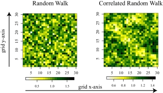
Figure 7: Spatial cost distributions generated by the random walk algorithms (Alg. 2 and 3). The two figures shows the $30\times 30$ grid cells with high cost cells in light and low cost cells in dark colors. The left figure was created by the random walk (algorithm 2) at $\Delta=5\cdot 10^{-5},\omega=0.0065$, to the right the correlated random walk (algorithm 3) at $\Delta=0.015,\omega=0.006$. Note that low and high cost areas are clustered for the correlated random walk.

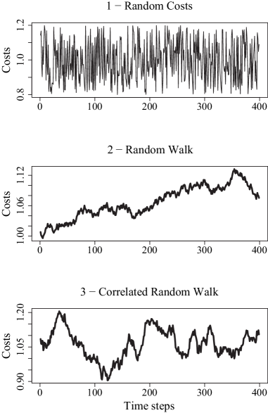
Figure 8: Time series of the costs of a grid cell over time. Algorithm 1 which changes costs randomly at each time step creates a strongly fluctuating time series. The two random walk algorithms lead to a time-correlated series.

Appendix B Model Scheduling

B.1 Economic Model

The economic model is initialized with a random configuration which is at the desired cost level. To ensure that the random walks are in a steady state, we ran the simulation 10000 time steps before the ecological model was initialized. Each time step, the scheduling was as follows:

Algorithm 4 Scheduling Economic Model

1:  Update costs

2:  repeat

3:     Adjust market price $P$

4:     for all cells do

5:        if $P\cdot\xi_{i}(l)>c_{i}(t)$ then

6:           $x_{i}=1$ (conserved)

7:        else

8:           $x_{i}=0$ (not conserved)

9:        end if

10:     end for

11:     Calculate ecological value and costs

12:  until budget constraint is met

13:  Update land configuration

B.2 Ecological Model

The ecological model was started by randomly choosing $60\%$ of the patches as occupied. We checked that populations were in a steady state after initialization and thus the measurements were not affected by the initialization (see Grimm and Wissel, 2004). The scheduling of the ecological model within one time step is as follows:

Algorithm 5 Scheduling Metapopulation Model

1:  for all populated cells do

2:     Local extinction with rate $e$

3:  end for

4:  for all populated cells do

5:     if Patch destroyed then

6:        Disperse with emigration rate $r_{d}$

7:     else

8:        Disperse with emigration rate $r$

9:     end if

10:  end for

11:  for all unpopulated cells do

12:     Check if immigration succesfull

13:  end for

References

- Ando et al. (1998) Ando, A., Camm, J., Polasky, S., Solow, A., 1998. Species distributions, land values, and efficient conservation. Science 279 (5359), 2126–2128.
- Bruggeman and Jones (2008) Bruggeman, D., Jones, M., 2008. Should habitat trading be based on mitigation ratios derived from landscape indices? A model-based analysis of compensatory restoration options for the red-cockaded woodpecker. Environmental Management 42 (4), 591–602.
- Chomitz (2004) Chomitz, K. M., 2004. Transferable development rights and forest protection: An exploratory analysis. International Regional Science Review 27 (3), 348–373.
- Chomitz et al. (2006) Chomitz, K. M., da Fonseca, G. A. B., Alger, K., Stoms, D. M., Honzak, M., Landau, E. C., Thomas, T. S., Thomas, W. W., Davis, F., 2006. Viable reserve networks arise from individual landholder responses to conservation incentives. Ecology and Society 11 (2), 40.
- Coggan and Whitten (2005) Coggan, A., Whitten, S. M., 2005. Market Based Instruments (MBIs) in Australia: What are they, important issues to consider and some applications to date. Tech. rep., CSIRO, accessed 29.11.2008.
- Drechsler and Wätzold (in press) Drechsler, M., Wätzold, F., in press. Applying tradable permits to biodiversity conservation: Effects of space-dependent conservation benefits and cost heterogeneity on habitat allocation. Ecological Economics.
- Drechsler et al. (2007) Drechsler, M., Wätzold, F., Johst, K., Bergmann, H., Settele, J., 2007. A model-based approach for designing cost-effective compensation payments for conservation of endangered species in real landscapes. Biological Conservation 140 (1-2), 174–186.
- EU-Commission (2007) EU-Commission, 2007. Green paper on market-based instruments for environment and related policy purposes. Tech. rep., Commission of the European Communities, accessed 29.11.2008.
- Fahrig (2002) Fahrig, L., 2002. Effect of habitat fragmentation on the extinction threshold: A synthesis. Ecological Applications 12 (2), 346–353.
- Ferraro and Kiss (2002) Ferraro, P. J., Kiss, A., 2002. Direct payments to conserve biodiversity. Science 298 (5599), 1718–1719.
- Ferraro and Pattanayak (2006) Ferraro, P. J., Pattanayak, S. K., 2006. Money for nothing? A call for empirical evaluation of biodiversity conservation investments. PLoS Biology 4 (4), E105.
- Fox and Nino-Murcia (2005) Fox, J., Nino-Murcia, A., 2005. Status of species conservation banking in the United States. Conservation Biology 19 (4), 996–1007.
- Grimm and Wissel (2004) Grimm, V., Wissel, C., 2004. The intrinsic mean time to extinction: A unifying approach to analysing persistence and viability of populations. Oikos 105 (3), 501–511.
- Hanski (1998) Hanski, I., 1998. Metapopulation dynamics. Nature 396, 41–49.
- Hanski (1999) Hanski, I., 1999. Metapopulation Ecology. Oxford University Press.
- Hanski et al. (1996) Hanski, I., Moilanen, A., Gyllenberg, M., 1996. Minimum viable metapopulation size. American Naturalist 147 (4), 527–541.
- Hartig and Drechsler (2008) Hartig, F., Drechsler, M., 2008. The time horizon and its role in multiple species conservation planning. Biological Conservation 141 (10), 2625–2631, arXiv:0807.4040.
- Hartig and Drechsler (submitted) Hartig, F., Drechsler, M., submitted. Stay by thy neighbor? Structure formation, coordination and costs in tradable permit markets with spatial trading rules, arXiv:0808.0111.
- Jack et al. (2008) Jack, B. K., Kousky, C., Sims, K. R. E., 2008. Designing payments for ecosystem services: Lessons from previous experience with incentive-based mechanisms. Proceedings of the National Academy of Sciences 105 (28), 9465–9470.
- Latacz-Lohmann and Schilizzi (2005) Latacz-Lohmann, U., Schilizzi, S., 2005. Auctions for conservation contracts: A review of the theoretical and empirical literature. Tech. rep., Report to the Scottish Executive Environment and Rural Affairs Department.
- Latacz-Lohmann and Van der Hamsvoort (1998) Latacz-Lohmann, U., Van der Hamsvoort, C. P. C. M., 1998. Auctions as a means of creating a market for public goods from agriculture. Journal of Agricultural Economics 49 (3), 334–345.
- Margules and Pressey (2000) Margules, C. R., Pressey, R. L., 2000. Systematic conservation planning. Nature 405 (6783), 243–253.
- Mills (1980) Mills, D. E., 1980. Transferable development rights markets. Journal of Urban Economics 7 (1), 63–74.
- Moilanen (2005) Moilanen, A., 2005. Reserve selection using nonlinear species distribution models. American Naturalist 165 (6), 695–706.
- Nelson et al. (2008) Nelson, E., Polasky, S., Lewis, D. J., Plantinga, A. J., Lonsdorf, E., White, D., Bael, D., Lawler, J. J., 2008. Efficiency of incentives to jointly increase carbon sequestration and species conservation on a landscape. Proceedings of the National Academy of Sciences of the United States of America 105 (28), 9471–9476.
- Nicholson and Possingham (2006) Nicholson, E., Possingham, H. P., 2006. Objectives for multiple-species conservation planning. Conservation Biology 20 (3), 871–881.
- Panayotou (1994) Panayotou, T., 1994. Conservation of biodiversity and economic development: The concept of transferable development rights. Environmental & Resource Economics 4 (1), 91–110.
- Polasky et al. (2008) Polasky, S., Nelson, E., Camm, J., Csuti, B., Fackler, P., Lonsdorf, E., Montgomery, C., White, D., Arthur, J., Garber-Yonts, B., Haight, R., Kagan, J., Starfield, A., Tobalske, C., 2008. Where to put things? Spatial land management to sustain biodiversity and economic returns. Biological Conservation 141 (6), 1505–1524.
- Salzman and Ruhl (2000) Salzman, J., Ruhl, J. B., 2000. Currencies and the commodification of environmental law. Stanford Law Review 53 (3), 607–694.
- Saunders et al. (1991) Saunders, D. A., Hobbs, R. J., Margules, C. R., 1991. Biological consequences of ecosystem fragmentation: A review. Conservation Biology 5 (1), 18–32.
- Scheffer et al. (2001) Scheffer, M., Carpenter, S., Foley, J. A., Folke, C., Walker, B., 2001. Catastrophic shifts in ecosystems. Nature 413 (6856), 591–596.
- van Teeffelen et al. (2006) van Teeffelen, A., Cabeza, M., Moilanen, A., 2006. Connectivity, probabilities and persistence: Comparing reserve selection strategies. Biodiversity and Conservation 15 (3), 899–919.
- Wilcove and Lee (2004) Wilcove, D. S., Lee, J., 2004. Using economic and regulatory incentives to restore endangered species: Lessons learned from three new programs. Conservation Biology 18 (3), 639–645.
- Williams and Araujo (2000) Williams, P. H., Araujo, M. B., 2000. Using probability of persistence to identify important areas for biodiversity conservation. Proceedings of the Royal Society of London Series B-Biological Sciences 267 (1456), 1959–1966.
- Wunder (2007) Wunder, S., 2007. The efficiency of payments for environmental services in tropical conservation. Conservation Biology 21 (1), 48–58.