Traveling spatially periodic forcing of phase separation

Abstract

We present a theoretical analysis of phase separation in the presence of a spatially periodic forcing of wavenumber $q$ traveling with a velocity $v$. By an analytical and numerical study of a suitably generalized 2d-Cahn-Hilliard model we find as a function of the forcing amplitude and the velocity three different regimes of phase separation. For a sufficiently large forcing amplitude a spatially periodic phase separation of the forcing wavenumber takes place, which is dragged by the forcing with some phase delay. These locked solutions are only stable in a subrange of their existence and beyond their existence range the solutions are dragged irregularly during the initial transient period and otherwise rather regular. In the range of unstable locked solutions a coarsening dynamics similar to the unforced case takes place. For small and large values of the forcing wavenumber analytical approximations of the nonlinear solutions as well as for the range of existence and stability have been derived.

1 Introduction

When a binary mixture at a critical composition is quenched from a homogeneous and usually high temperature phase sufficiently below the coexistence curve then inhomogeneous concentration variations of a characteristic average domain size occur which are known as spinodal decomposition (SD) Gunton:83.1 ; Bray:94.1 . With the progress of time a coarsening process takes place, i.e. the average domain size increases continuously. The dynamics of phase separation under homogeneous conditions has been intensively studied for numerous systems during the recent decades Gunton:83.1 ; Bray:94.1 . In this work we explore the effects of a traveling spatially periodic forcing on phase separation.

For several kinetic mechanisms associated with first order phase transitions, such as nucleation and growth, thermal activation energy is required, but not for SD. The order parameter, that describes the phase separation in binary mixtures, is the local composition (concentration) and it obeys a local conservation law. Hence in phase separating systems the order parameter is a conserved one in contrast to the large number of pattern forming systems, where one has to deal with non-conserved order parameters CrossHo . The phase separation is limited by diffusion-like processes and therefore in its late stage, where small inhomogeneities have developed into macroscopic domains, the decomposition dynamics becomes rather slow.

Phase separation is also employed in producing technologically important functional elements in e.g. lithographic processes, biosensors and semiconductor devices Walheim:1999.1 ; Boeltau:1998.1 ; Voeroes:2005.1 ; Sirringhaus:2005.1 . Therefore, an understanding of the mechanisms of the formation of regular structures is highly important for technological applications and even the control of regular patterns is desired.

In a large number of investigations the effects of external fields on phase separation have been examined, such as for instance the effects of shear flow Berthier:2001.1 , time-dependent temperature variation Tanaka:1995.1 or local Krekhov:2005.1 as well as spatially periodic heating Krekhov:2004.1 . In the presence of spatially periodic forcing coarsening can be interrupted above a critical modulation amplitude and locked solutions can be found Krekhov:2004.1 .

Especially for pattern forming systems with non-conserved order parameters external forcing has been recognized as a powerful method for investigations of the response behavior of nonlinear patterns and of the inherently nonlinear mechanisms of selforganization. The effect of spatially periodic forcing on pattern formation has been investigated rather early in the context of thermal forcing Kelly:78.1 and electroconvection in nematic liquid crystals Lowe:83.1 ; Lowe:86.1 . Further on, the response of stationary patterns with respect to static spatially periodic forcing in one or two spatial dimensions has been explored with respect to modulated structures Lowe:83.1 ; Lowe:86.1 ; Coullet:86.2 ; Coullet:87.1 ; Coullet:89.1 ; Zimmermann:93.3 ; Zimmermann:96.1 ; Kai:1999.1 ; Ribotta:2003.1 or with respect to induced time-dependent phenomena Rehberg:91.2 ; Zimmermann:96.2 ; Zimmermann:96.3 . Separately also the effects of temporal forcing have been investigated Riecke:88.1 ; Walgraef:88.1 ; Rehberg:88.1 ; Swinney:2000.1 ; Swinney:2000.2 . Recently a number of new phenomena have been found and explored by a combination of spatial and temporal forcing in model systems Krekhov:2008.1 ; Zimmermann:2002.2 ; Sagues:2003.1 ; Kramer:2004.1 ; Schuler:2004.1 ; Ruediger:2007.1 ; Ruediger:2007.2 . Here we present the first investigation of the effects of pulled spatially periodic external forcing on a pattern forming model system with a conserved order parameter.

The paper is organized as follows. In Sec. 2 we present the model equation for the conserved order parameter field. In section 3 the one-dimensional periodic solutions and their existence range are described and their linear stability analysis in one and two dimensions is presented in section 4. The results of numerical simulations of the dynamics of phase separation under traveling spatially periodic forcing in 1D and 2D are given in Sec. 5. Some concluding remarks are added in Sec. 6. In the Appendix we describe the condition for the existence of spatially periodic solutions and analytical approximations for the solutions in the limit of small and large values of the forcing wavenumber.

2 Model

A model for phase separation in various systems is the Cahn-Hilliard equation for a conserved order parameter field $\psi(\mathbf{r},t)$ representing the local concentration of one of the components of a binary mixture. Here we focus on the effects of traveling spatially periodic forcing on phase separation as described by the modified Cahn-Hilliard equation

$$\partial_{t}\psi(\mathbf{r},t)=\nabla^{2}\{-\varepsilon\psi+\psi^{3}-\nabla^{2}\psi+a\cos[q(x-vt)]\}.$$ (1)

The forcing term $a\cos[q(x-vt)]$ is caused by an interplay between a traveling temperature modulation and thermal diffusion (Soret effect). Its derivation has been described in detail for $v=0$ in Ref. Krekhov:2004.1 . Such a traveling spatially periodic temperature modulation could be created for instance in optical grating experiments Wiegand:2002.1 ; Wittko:2003.1 with a light intensity $I(x,t)\sim\cos[q(x-vt)]$. The control parameter $\varepsilon$ in Eq. (1) corresponds to a dimensionless distance to the critical temperature of the binary mixture. A transformation of Eq. (1) in the frame comoving with the traveling forcing $x\rightarrow x-vt$ gives

$$\partial_{t}\psi(\mathbf{r},t)=\nabla^{2}[-\varepsilon\psi+\psi^{3}-\nabla^{2}\psi+a\cos(qx)]+v\,\partial_{x}\psi.$$ (2)

3 Periodic solutions and bifurcation diagrams in 1D

During the initial stage of an unforced phase separation, i.e. $a=0$ and $v=0$, small perturbations of the homogeneous solution $\psi=0$ exhibit an exponential growth for $\varepsilon>0$ and the growth rate $\sigma=k^{2}(\varepsilon-k^{2})$ shows a maximum at a distinguished wavenumber $k_{m}=\sqrt{\varepsilon/2}$. Beyond the regime of exponential growth one observes the well known coarsening dynamics of phase separation.

If phase separation is forced by a spatially periodic temperature modulation the coarsening dynamics is interrupted beyond a critical value of the forcing amplitude $a$ and it is locked to the periodicity of the external forcing Krekhov:2004.1 . However, if this forcing is pulled by a velocity $v\not=0$, the spatially periodic solutions do exist only in a certain range of $v$ depending on $a$. The conditions for the existence of spatially periodic solutions are formulated in Appendix A.1 and they are explicitely calculated for various parameters in this section.

The bifurcation diagrams of spatially periodic solutions of Eq. (2) are described for $v=0$ in subsection 3.2 as well as for $v\neq 0$ in 3.3 and the numerical method for calculating the solutions is explained in subsection 3.1.

3.1 Numerical solution

The stationary $2\pi/q$-periodic solutions of Eq. (2) can be represented by a truncated Fourier expansion

$$\psi_{s}(x)=\sum\limits_{k=-N}^{N}C_{k}e^{iqxk}$$ (3)

with time-independent Fourier coefficients $C_{-k}=C_{k}^{*}$. Using this ansatz one obtains after projection of Eq. (2) onto the $j$-th Fourier mode ($\int_{0}^{2\pi/q}e^{-iqxj}dx$), the coupled system of nonlinear inhomogeneous equations for the corresponding expansion coefficients $C_{j}$

$$[\varepsilon(jq)^{2}-(jq)^{4}+ivjq]C_{j}-\frac{aq^{2}}{2}(\delta_{1,j}+\delta_{-1,j})$$

$$\qquad-(jq)^{2}\sum\limits_{k,l}C_{k}C_{l}C_{j-k-l}=0\,,\,\,\,\,\,\,j=-N..N,$$ (4)

which has been solved by Newton’s method. $N$ was adjusted in order to keep a relative error smaller than $10^{-6}$ (e.g. $N=81$ for $q=0.5$).

3.2 Periodic solutions for $v=0$

For positive values of $\varepsilon$ spatially periodic solutions of Eq. (2) may be found with and without forcing. However, in the unforced case ($a=0$) Eq. (2) has a $\pm\psi$-symmetry and therefore one has a pitchfork bifurcation from the trivial solution $\psi=0$ to finite amplitude periodic solutions as indicated by the dotted line in Fig. 1. For $a=0$ periodic solutions are unstable for any wavenumber $q$ against coarsening with the fastest growing mode as period doubling Langer:71.1 ; Krekhov:2004.1 .

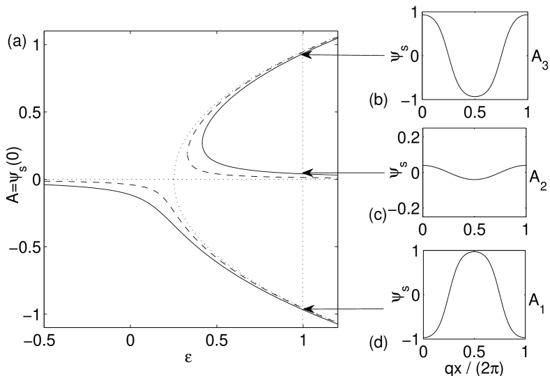
Figure 1: Part (a) shows the bifurcation diagram for spatially periodic solutions at a forcing wavenumber $q=0.5$ and modulation amplitudes $a=0$ (dotted), $a=0.01$ (dashed) and $a=0.03$ (solid). Parts (b), (c) and (d) show the three solutions $\psi_{s}(x)$ over one period corresponding to the different branches of the bifurcation diagram for $a=0.03$ and $\varepsilon=1$.

For finite values of the modulation amplitude $a$ the $\pm\psi$-symmetry is broken as indicated in Fig. 1 for $a=0.01$ by the dashed line and for $a=0.03$ by the solid line. While we have in the unmodulated case a trivial solution $\psi=0$ and two finite solutions with identical amplitudes but of opposite sign, one finds in the forced case three periodic solutions, $A_{1}$, $A_{2}$ and $A_{3}$, of different amplitude as shown in Fig. 1 (b)-(d). The $A_{3}$- and $A_{2}$-solutions are in phase with the external modulation and the preferred $A_{1}$-solution is shifted by half a period.

The amplitudes of the $A_{1}$- and the $A_{3}$-solution increase with increasing values of the control parameter $\varepsilon$, but they also depend on $q$ and $a$. For a given modulation amplitude $a$ the amplitude of $A_{1}$ decreases with increasing values of the modulation wavenumber $q$ as indicated in Fig. 2. This trend holds also for the $A_{3}$-solution but the amplitude of the $A_{2}$-solution increases with $q$.

Keeping $q$ fixed and increasing the modulation amplitude $a$ the amplitude of the $A_{1}$-solution increases as can be seen in Fig. 1. This also holds for the $A_{2}$-solution. In contrast to this trend, the amplitude of the $A_{3}$-solution decreases with increasing values of $a$ (see dashed and solid lines in Fig. 1). In case of small $q$ (long wavelength modulation) the solutions $A_{1}$ and $A_{3}$ become steplike as shown in Fig. 2 (a) for $A_{1}$. This steplike shape also occurs, if the control parameter $\varepsilon$ becomes rather large compared to the modulation amplitude. The shape of the $A_{2}$-solution does not change when $a$ or $\varepsilon$ are varied.

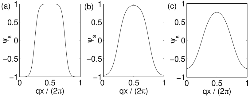
Figure 2: $A_{1}$-solution for different values of the modulation wavenumber: $q=0.25$ (a), $q=0.5$ (b) and $q=0.75$ (c). The other parameters are $\varepsilon=1$, $v=0$ and $a=0.01$.

3.3 Periodic solutions for $v\not=0$

The nonlinear solutions and the bifurcation diagram as given in Fig. 1 are only slightly changed by a finite traveling velocity. However, with increasing values of $v$ a phase shift $\Delta\phi$ between the periodic forcing $\sim\cos(qx)$ and the solution $\psi_{s}(x)$ occurs. This is shown in Fig. 3 for three different values of $v$ for both the $A_{1}$- and the $A_{3}$-solution. The $A_{1}$-solution, which is in antiphase with the external modulation, drags behind the forcing ($\Delta\phi>0$). This delay increases with increasing values of $v$ (all other parameters fixed). The maximum phase shift that can be achieved is about $\Delta\phi_{m}=\pi/2$ at a certain velocity $v_{ex}$ above which the solution does not exist. In contrast to this behavior the $A_{3}$-solution has a negative phase shift $\Delta\phi<0$ with respect to the forcing as indicated by the lower part in Fig. 3. The maximum absolute value of the phase shift in this case is also $\pi/2$. As indicated in Fig. 4 (b) the critical phase shift $\Delta\phi_{m}=\pi/2$ for the $A_{1}$-solution is reached with an increasing value of the velocity $v$ at lower values of the control parameter $\varepsilon$.

For a fixed $\varepsilon$ a velocity $v_{ex}$ can be determined by the $\pi/2$-criterion where both the $A_{1}$- and the $A_{3}$-solution vanish to exist whereas the $A_{2}$-solution still exists and propagates ahead of the external modulation with the absolute value of the phase shift always smaller than $\pi/2$. However, as will be shown later, this solution is always unstable.

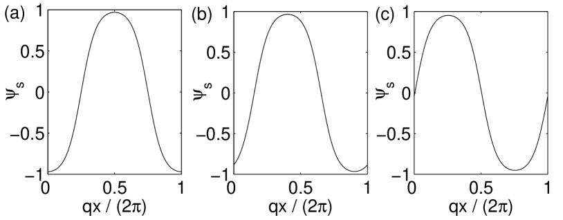
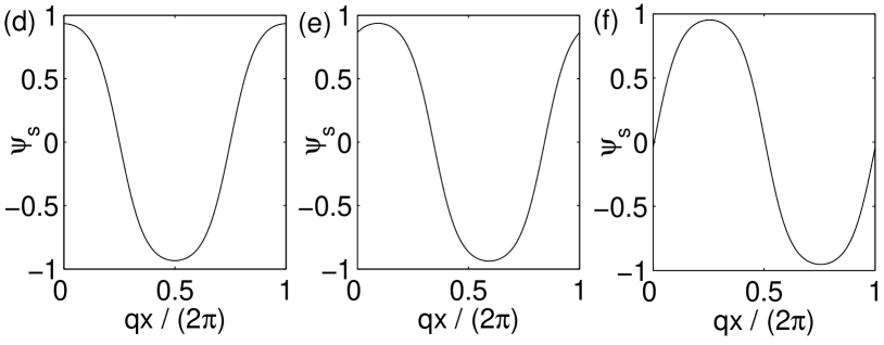
Figure 3: $A_{1}$-solution (top) and $A_{3}$-solution (bottom) for the velocity $v=0$ (a,d), $v=0.008$ (b,e) and $v=0.0142$ (c,f). The other parameters are $q=0.5$, $a=0.03$ and $\varepsilon=1$.

The amplitudes for the three solutions $A_{i}$ ($i=1,2,3$) are plotted as a function of the control parameter $\varepsilon$ for four different values of the propagation velocity $v$ in the bifurcation diagram in Fig. 4. As can be seen in this plot, the amplitudes for all four velocities are nearly identical.

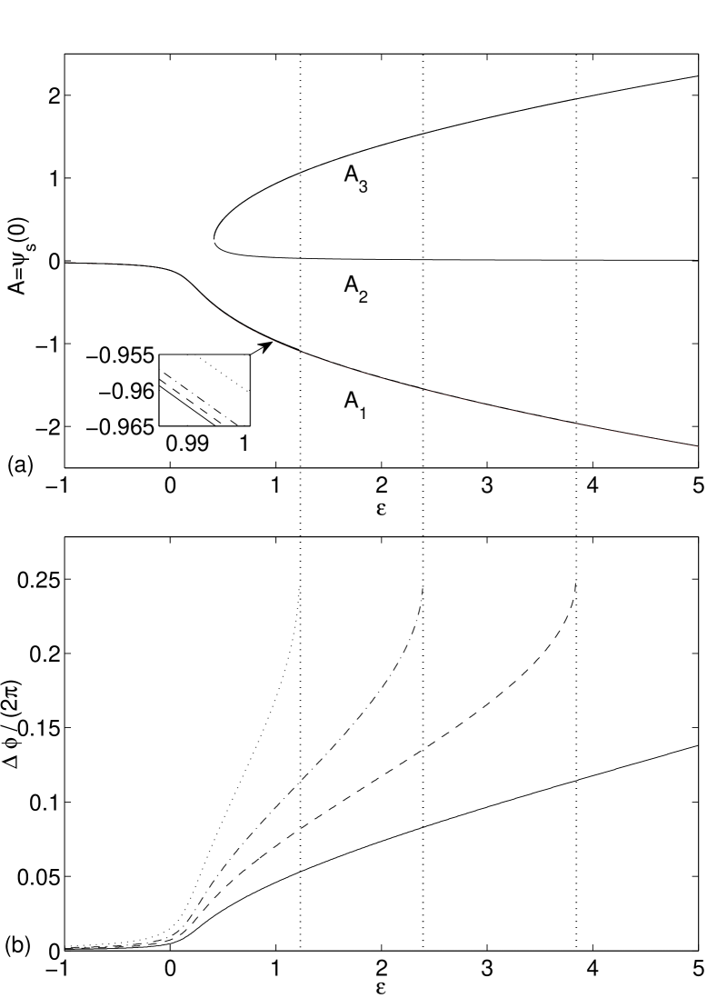
Figure 4: The bifurcation diagram for $q=0.5$, $a=0.03$ and finite values of the velocity $v$ is shown in (a) and in (b) the phase shift $\Delta\phi/(2\pi)$ of the $A_{1}$-solution is presented for different velocities: $v=0.004$ (solid), $v=0.006$ (dashed), $v=0.008$ (dashed-dotted) and $v=0.0142$ (dotted).

The shape of the solution $\psi_{s}$ becomes steplike for small values of $q$, as indicated in Fig. 2 (a). In the range $q\lesssim 0.3$ the solution can be approximated rather well by a series of hyperbolic tangents as shown in Appendix A.2. In the opposite case $q>0.5$ one can achieve a rather good approximation of the periodic solution by restricting the Fourier ansatz in Eq. (3) to the leading modes as explained in Appendix A.3.

4 Stability of periodic solutions in 1D and 2D

The stationary periodic solutions $\psi_{s}(x)$ of Eq. (2) studied so far are stable only in a subrange of parameters where they exist. In this section we investigate the stability of periodic solutions $\psi_{s}(x)$ of Eq. (2) with respect to small perturbations. The resulting linear partial differential equation for the perturbation $\psi_{1}$

$$\partial_{t}\psi_{1}(x,t)=\partial_{x}^{2}\left(-\varepsilon+3\psi_{s}^{2}-\partial_{x}^{2}\right)\psi_{1}+v\partial_{x}\psi_{1}$$ (5)

contains a spatially periodic coefficient depending on $\psi_{s}$. Accordingly the solutions of Eq. (5) are due to the Floquet theory of the form

$$\psi_{1}(x,t)=e^{\sigma t}~{}e^{isx}~{}\phi_{F}(x)\,,$$ (6)

with the Floquet parameter $s$ and a $2\pi/q$-periodic function $\phi_{F}(x)$. This periodic function $\phi_{F}(x)$ can be represented by a Fourier expansion

$$\phi_{F}(x)=\sum_{n=-N}^{N}~{}D_{n}~{}e^{iqxn}.$$ (7)

Taking into account Eq. (3) for $\psi_{s}$ the linear partial differential equation (5) is transformed into an eigenvalue problem

$$\sigma D_{l} = \left[\varepsilon(ql+s)^{2}-(ql+s)^{4}+iv(ql+s)\right]D_{l}$$ (8)

$$-3(ql+s)^{2}\sum_{k,m}C_{k}C_{m}D_{l-k-m}\,,\,\,\,\,\,\,l=-N..N,\qquad$$

with the coefficients $C_{k}$ determined by Eq. (4).

The growth rate $\sigma$ for the solutions $A_{1}$, $A_{2}$ and $A_{3}$ is shown in Fig. 5 as function of the Floquet parameter $s$ for three different values of the velocity $v$ and fixed values of the forcing amplitude $a$, the forcing wavenumber $q$ and the control parameter $\varepsilon$.

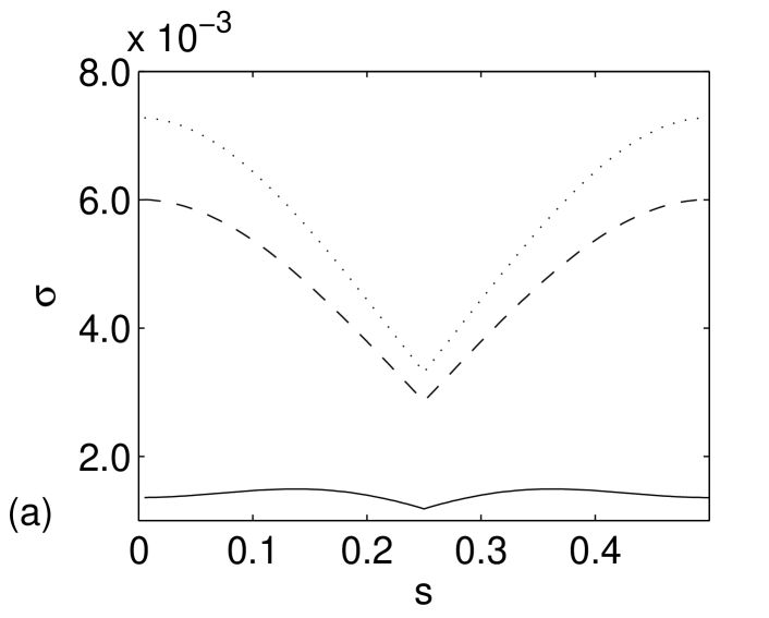
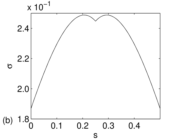
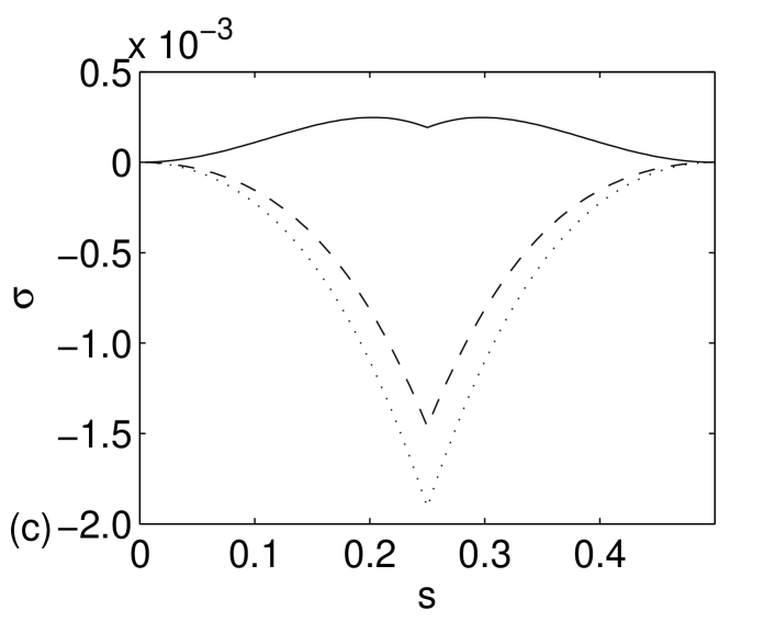
Figure 5: The growth rate $\sigma$ of small perturbations with respect to the stationary periodic solution is shown as a function of the Floquet parameter $s$ for the $A_{1}$ (a), the $A_{2}$ (b) and the $A_{3}$-solution (c) for the three propagation velocities $v=0$ (dotted), $v=0.008$ (dashed) and $v=0.014$ (solid). Further parameters are $q=0.5$, $a=0.03$ and $\varepsilon=1$. In case of the $A_{2}$-solution all three lines are indistinguishable.

We found that for the solutions $A_{2}$ and $A_{3}$ the growth rate $\sigma$ is positive for all combinations of the parameters $\varepsilon$, $q$, $a$ and $v$. Accordingly $A_{2}$ and $A_{3}$ are always unstable. The growth rate of the perturbation of the $A_{1}$-solution is negative for certain parameter ranges, meaning that this is the only solution that can be stabilized. For fixed $\varepsilon$ and $q$ the modulation amplitude $a$ has to exceed a certain value $a_{s}(q)$ to stabilize the $A_{1}$-solution. If the traveling velocity $v$ is smaller than a critical one $v_{c}(\varepsilon,a,q)$ the solution remains stable. The critical velocity $v_{c}(\varepsilon,a,q)$ is given by the solid line in Fig. 6 for a certain set of parameters and for $v>v_{c}(\varepsilon,a,q)$ the periodic solutions are linearly unstable. The onset of instability occurs for small values of the Floquet exponent $s\rightarrow 0$, i.e. belongs to a long-wave perturbation. In Fig. 6 also the boundary of the existence range of periodic solutions $v_{ex}(\varepsilon,a,q)$ is shown as obtained approximately by Eq. (27) (dashed line) and by a full numerical simulation (dotted line). Since the stability boundary (solid line) always lies below $v_{ex}$ the periodic solution always becomes unstable before the existence range is reached.

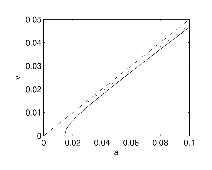
Figure 6: Above the solid line the spatially periodic solution is unstable. The dashed line marks the existence boundary above which the spatially periodic solution does not exist due to the criterion given by Eq. (27). The dotted curve marks the existence boundary obtained numerically from Eq. (4). The parameters are $q=0.5$ and $\varepsilon=1$.

Extending the analysis to two spatial dimensions the stability of a two-dimensional stripe pattern that is periodic in the $x$-direction can be investigated using $\psi(x,y,t)=\psi_{s}(x)+\psi_{2}(x,y,t)$ with $|\psi_{2}|<<|\psi_{s}|$. The procedure is the same as in one dimension whereas the perturbation $\psi_{2}(x,y,t)$

$$\psi_{2}(x,y,t)=e^{\sigma t}~{}e^{i(sx+py)}~{}\phi_{F}(x)\,,$$ (9)

depends now on two Floquet parameters $s$ ($x$-direction) and $p$ ($y$-direction). Linearizing Eq. (2) and using expansion (7) one obtains the eigenvalue problem

$$\sigma D_{l} = [\varepsilon(ql+s)^{2}+\varepsilon p^{2}-(ql+s)^{4}$$

$$-2(ql+s)^{2}p^{2}-p^{4}+iv(ql+s)]D_{l}$$

$$-3[(ql+s)^{2}+p^{2}]\sum_{k,m}C_{k}C_{m}D_{l-k-m}\,,\,\,l=-N..N.$$

The linear stability analysis shows that additional transversal degrees of freedom do not influence the stability diagram obtained for the one-dimensional case.

5 Dynamics of the phase separation

To study the temporal evolution of the phase separation numerical simulations of Eq. (1) for one and two spatial dimensions have been performed. We have used a central finite difference approximation of the spatial derivatives and an Euler integration of the resulting ordinary differential equations in time. Periodic boundary conditions have been used and we start initially with the homogeneous state $\psi=0$ with small superimposed noise.

5.1 1D Simulations

In one dimension we have discretized a system of length $L=24\,\pi/q$ by $N=200$ steps with a step size $\delta x=L/N$ and a time step $\Delta t=10^{-3}$. The noise amplitude for the initial condition $\psi=0$ was adjusted at $10^{-4}$. The evolution of the inhomogeneous pattern has been characterized by the structure factor at the modulation wavenumber $q$

$$S(q,t)=|\hat{\psi}(q,t)|^{2}\,,\,\hat{\psi}(q,t)=\int dxe^{iqx}\psi(x,t).$$ (11)

In the early stages of phase separation the amplitude of $S(q,t)$ grows faster for $v\neq 0$ and even exceeds its final value for some time as can be seen in Fig. 7.

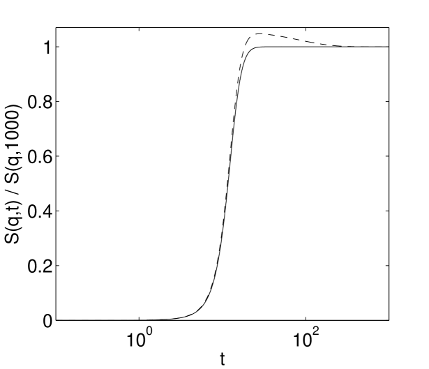
Figure 7: The dynamics of the maximum of the structure factor (relating to its final value) for $v=0$ (solid line) and $v=0.0266<v_{c}$ (dashed line). The other parameters are $\varepsilon=1$, $q=0.5$ and $a=0.1$.

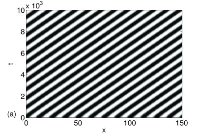
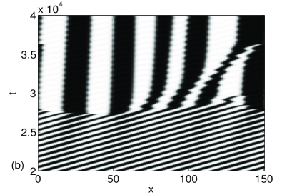
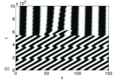
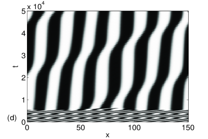
Figure 8: Temporal evolution of phase separation is shown for $v=0.015<v_{c}$ (a), $v_{c}<v=0.0185<v_{ex}$ (b) and $v=0.02>v_{ex}$ (c,d). The other parameters are $\varepsilon=1$, $a=0.04$ and $q=0.5$.

The temporal evolution of $\psi(x,t)$ is shown in Fig. 8 for three velocity regimes. In part (a) of Fig. 8 the velocity is sufficiently small and belongs to the range where the pattern is locked to the propagating external modulation. In part (b) the velocity is chosen in the range $v_{c}<v=0.0185<v_{ex}$ where the solution locked to the traveling external modulation still exists, but where it is linearly unstable. In this parameter range the solution is locked during the initial period of phase separation before coarsening takes over. In parts (c) and (d) the temporal evolution of phase separation is shown for a velocity $v=0.02>v_{ex}$ where the locked solution does not exist anymore. At this velocity an interesting pinning-depinning behaviour can be observed during the initial stage of phase separation. One still has a travelling periodic solution with the same wavenumber as the forcing but with a velocity smaller than the velocity of the forcing. Due to the velocity mismatch the phase shift between the solution and the forcing is slowly increased before it reaches about half of the forcing period. From that moment the periodic solution practically stops moving (pinning) until the forcing shifts over the next half of the period. After that the solution starts moving again (depinning) and the process repeats itself a few times. Later on the agreement of the wavelengths of the solution and the forcing cannot be maintained anymore and the coarsening takes place.

5.2 2D Simulations

In two spatial dimensions the same system size as in 5.1 has been used in both directions, $L_{x}=L_{y}=24\,\pi/q$ with $N_{x}=N_{y}=256$ discretization points. Again we chose $10^{-4}$ as noise amplitude for the initial homogeneous state.
The numerical simulations in two dimensions are in agreement with the results of the linear stability analysis of Sec. 4.

Figure 9: Snapshot of the phase separation in 2d for $q=0.5$, $v=0.0188\,(\approx 1.07\cdot v_{c})$, $a=0.04$, $\varepsilon=1$ at $t=5\times 10^{4}$ (a) and for $q=0.75$, $v=0.266\,(\approx 1.32\cdot v_{c})$, $a=0.3$, $\varepsilon=1$ at $t=5\times 10^{3}$ (b). The curves at the bottom indicate the external forcing.

For $a>a_{c}$ and $v<v_{c}$ one obtains stable stripe patterns. In the unstable range $v>v_{c}$ the locking of the solution gets lost and a coarsening sets in as shown in Fig. 9 (a) for $v\approx 1.07\cdot v_{c}$ slightly beyond the critical velocity and in Fig. 9 (b) for $v=0.266$ ($\approx 1.32\cdot v_{c}$). For $v>v_{c}$ the linear stability analysis of the locked solutions in two spatial dimensions shows that transversal perturbations being periodic in the $y$-direction exhibit also a positive growth rate $\sigma(s,p)$. However, for small values of the forcing wavenumber $q$, the modulational wavenumber $p$ is very small and the corresponding length $2\pi/p$ may be larger than the system size in our simulations. In this case the coarsening is quasi-one-dimensional along the $x$-direction as can be seen for instance in Fig. 9 (a). For larger values of $q$ also the length scale $2\pi/p_{c}$, with $p_{c}$ at the maximum of the growth rate $\sigma(s,p)$, becomes smaller than the system length $L_{y}$. In this parameter range the coarsening shows a two-dimensional behaviour as shown in Fig. 9 (b).

6 Summary and conclusions

Effects of a spatially periodic forcing, which travels with velocity $v$, on phase separation in binary mixtures have been investigated in terms of a generalized Cahn-Hilliard model. For a sufficiently large forcing amplitude we identified three characteristic velocity regimes which are distinguished by the different evolving pattern and their dynamics. For a vanishing velocity $v$ and the forcing amplitude $a$ larger than a critical value $a_{c}$ the phase separation can be locked to the external modulation Krekhov:2004.1 .

For a finite velocity $v$ a condition is derived in Appendix A.1 which determines the parameter range where the spatially periodic solutions of the same wavelength as the external forcing exist. This spatially periodic solution is locked with respect to the external forcing in a finite parameter range beyond $a>a_{c}$ and it is dragged by the forcing with some phase delay. This phase delay increases with the velocity $v$ up to some critical value $v_{ex}$. Beyond $v_{ex}$ the locked spatially periodic solution does not exist anymore as described in Section 3.3 and as shown by Fig. 4.

In the limit of small values of the modulation wavenumber $q$ the forced solutions resemble a periodic array of kinks and may be approximated by a series of hyperbolic tangents as given by Eq. (16). For this approximate solution we derived in Appendix A.2 with the help of the existence condition given in Appendix A.1 an analytical expression for the boundary of the parameter range of existence of the locked solutions. Also in the range of larger values of $q$ an analytical approximation of the nonlinear solution as well as its boundary of the existence range has been determined in Appendix A.3.

The locked and dragged spatially periodic solutions are linearly stable only in a subdomain of their range of existence as described in Section 4. The critical velocity $v_{c}(\varepsilon,a,q)$, beyond which the locked solutions become unstable and a depinning of the locked solutions takes place, is given as function of $a$ in Fig. 6. For large values of $q$ the numerical results of the stability analysis have been compared with results of an analytical approximation in Appendix A.3, cf. Fig. 11.

In the parameter range of unstable locked solutions one observes in the two phase region a coarsening dynamics rather similar to the coarsening in the unforced case. However, during an initial transient period the nonlinear evolution of the solutions is different in the parameter range where the locked solutions still exist from that where they do not exist anymore. In the former case they are just locked during a transient period to the traveling forcing and in the latter case irregular phase jumps occur.

In the range, where the locked solutions are either unstable or do not exist, we observe for finite values of the traveling velocity $v$ a faster coarsening dynamics than in the limit $v=0$.

The analysis presented here shows that travelling spatially periodic forcing can serve as an effective tool for the control of phase separation. The finite velocity of the forcing leads to a faster dynamics of the initial stage of phase separation compared to the case of a stationary spatially periodic forcing. The results should be relevant to thin polymer blends with a moderate Soret coefficient and a weak periodic temperature modulation created, e.g., by means of optical grating techniques.

Appendix A Stationary periodic solutions

A.1 Existence of spatially periodic solutions

The condition of existence of stationary periodic solutions $\psi_{s}(x)$ of Eq. (2) with the wavenumber $q$ of the external forcing is derived in this section. $\psi_{s}(x)$ is a solution of the following equation

$$0=\partial_{x}^{2}[-\varepsilon\psi_{s}+\psi_{s}^{3}-\partial_{x}^{2}\psi_{s}+a\cos(qx)]+v\,\partial_{x}\psi_{s}.$$ (12)

Assuming $\psi_{s}(x)$ being a periodic function with a vanishing mean value $\int_{0}^{2\pi/q}\psi_{s}(x^{\prime})dx^{\prime}=0$ one obtains after two integrations of Eq. (12)

$$\partial_{x}\left\{-\varepsilon\frac{1}{2}\psi_{s}^{2}+\frac{1}{4}\psi_{s}^{4}-\frac{1}{2}(\partial_{x}\psi_{s})^{2}\right\}+a\cos(qx)(\partial_{x}\psi_{s})$$

$$\qquad+v\,(\partial_{x}\psi_{s})\int\limits_{0}^{x}\psi_{s}(x^{\prime})dx^{\prime}=C\,(\partial_{x}\psi_{s}).$$ (13)

Using again the periodicity of $\psi_{s}$, an integration of (LABEL:help2eq) with respect to the interval $[0,2\pi/q]$ gives

$$0=\int\limits_{0}^{2\pi/q}dx\left[a\cos(qx)(\partial_{x}\psi_{s})+v(\partial_{x}\psi_{s})\int\limits_{0}^{x}\psi_{s}(x^{\prime})dx^{\prime}\right].$$ (14)

After an integration by parts of (14) the constraint of existence for stationary periodic solutions $\psi_{s}(x)$ of Eq. (2) follows:

$$0=aq\int\limits_{0}^{2\pi/q}\sin(qx)\psi_{s}(x)dx-v\int\limits_{0}^{2\pi/q}\psi_{s}^{2}(x)dx.$$ (15)

A.2 Analytical approximation in the limit of small $q$

For small values of the wavenumber $q$ the solutions for the $A_{1}$-branch become steplike periodic functions as indicated in Fig. 2 (a). Kink-type periodic functions may be approximated by a series of hyperbolic tangents Langer:71.1

$$\psi_{s}(x)=\sqrt{\varepsilon}\cdot\sum_{n=0}^{N}(-1)^{n}\tanh\left[M(x)\right]$$ (16)

where

$$M(x)=\sqrt{\frac{\varepsilon}{2}}~{}\left[x-(n+\frac{1}{2})\frac{\pi}{q}+\gamma\right]$$ (17)

describing a periodic array of $N$ single interfaces with a spacing $\pi/q$ (size of the system $L=N\cdot\pi/q$). $\gamma$ depends on $q,~{}\varepsilon,~{}a$ and $v$. Inserting the ansatz (16) into Eq. (15) one obtains

$$\int\limits_{0}^{2\pi/q}\sin(qx)\cdot\sqrt{\varepsilon}\sum_{n=0}^{N}(-1)^{n}\tanh\left[M(x)\right]dx$$

$$\quad=\frac{v}{aq}\int\limits_{0}^{2\pi/q}\Bigg{[}\sqrt{\varepsilon}\sum_{n=0}^{N}(-1)^{n}\tanh\left[M(x)\right]\Bigg{]}^{2}dx$$ (18)

for the determination of $\gamma$, which may be reformulated in the following form

$$\int\limits_{0}^{2\pi/q}\sin(qx)\cdot\sum_{n=0}^{N}(-1)^{n}\tanh\left[M(x)\right]dx$$

$$\quad\quad=\frac{v\sqrt{\varepsilon}}{aq}\Bigg{\{}\frac{2\pi}{q}-\int\limits_{0}^{2\pi/q}\sum_{n=0}^{N}\mbox{sech}^{2}\left[M(x)\right]dx\Bigg{\}}.\qquad$$ (19)

For $q\ll 1$ the first integral in this equation may be approximated by the expression

$$\int\limits_{0}^{2\pi/q}\sin(qx)\cdot\sum_{n=0}^{N}(-1)^{n}\tanh\left[M(x)\right]dx\approx\frac{4}{q}\sin(\gamma q)$$

and the second integral by

$$\int\limits_{0}^{2\pi/q}\sum_{n=0}^{N}\mbox{sech}^{2}\left[M(x)\right]dx\approx 4\sqrt{\frac{2}{\varepsilon}}\,.$$ (21)

Both integrals together with Eq. (19) give an explicit expression for the constant $\gamma$

$$\gamma=\frac{1}{q}\mbox{arcsin}\left[\frac{v\sqrt{\varepsilon}}{a}\left(\frac{\pi}{2q}-\sqrt{\frac{2}{\varepsilon}}\right)\right]$$ (22)

in terms of the parameters of the external forcing. With $\gamma$ as determined above the representation in Eq. (16) is a good approximation of the solution as it deviates less than 10% from the full numerical solution for $q\lesssim 0.3$. The deviation decreases with decreasing $q$.

In the range of the coexistence of the three branches $A_{1}$, $A_{2}$ and $A_{3}$ the shift $\gamma$ between the forcing and the spatially periodic solution increases with an increasing velocity $v$ up to the numerically determined existence limit of the $A_{1}$-solution at approximately $\gamma q=\Delta\phi_{m}=\pi/2$, as described in Sec. 3.3. With this condition $\gamma q=\pi/2$ we may also calculate the velocity

$$v_{ex}=\frac{2aq}{\pi\sqrt{\varepsilon}-2q\sqrt{2}}$$ (23)

below which the periodic kink-type solution exists. This analytical expression for $v_{ex}$ is in a good agreement with the numerically determined existence boundary.

A.3 Analytical approximation in the limit of large $q$

For large $q$ the nonlinear solution can be described by a leading order Fourier expansion: $\psi_{s}\propto\cos(qx)$. However, if the forcing is propagating with a velocity $v$ a phase shift between the forcing and the periodic solution $\psi_{s}(x)$ occurs and this phase shift can be taken into account by the following ansatz:

$$\psi_{s}(x)=C_{1}\cos(qx)+C_{2}\,v\sin(qx).$$ (24)

This corresponds to a restriction of the series given by Eq. (3) to $N=1$. Inserting the ansatz (24) in Eq. (12) and collecting the linear independent contributions proportional to $\sin(qx)$ and $\cos(qx)$ one obtains the two coupled equations for the coefficients $C_{1}$ and $C_{2}$

$$\left(\varepsilon-q^{2}-\frac{3}{4}\,C_{1}^{2}-\frac{3v^{2}}{4}\,C_{2}^{2}\right)C_{1}\,+\frac{v^{2}}{q}\,C_{2}-a = 0,$$ (25)

$$\left(\varepsilon-q^{2}-\frac{3v^{2}}{4}\,C_{2}^{2}-\frac{3}{4}\,C_{1}^{2}\right)C_{2}-\frac{1}{q}\,C_{1} = 0.$$ (26)

In the range $q>0.5$ a numerical solution of these two coupled equations provides solutions which deviate less than 30% from the full numerical solution.

The deviation decreases further with increasing $q$. A comparison between the solution (24) and the full numerical solution is shown in Fig. 10 for $q=0.5$. The deviations increase at larger values of $\varepsilon$ and close to the boarder where the stationary solutions vanish to exist.

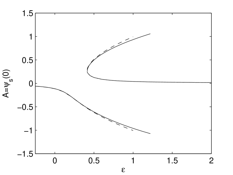
Figure 10: The bifurcation diagram obtained from the full numerical solution (solid) and the approximation (24) (dashed) for the parameters $q=0.5$, $a=0.03$ and $v=0.01424$.

The existence range of the $A_{1}$-solution again may be determined by assuming a maximum phase shift of $\pi/2$ between the external forcing and the periodic solution. In this case the $\cos$-contribution in Eq. (24) vanishes, that means one should have $C_{1}=0$. Then the velocity $v_{ex}$ can be calculated from the existence of the solution $C_{2}\neq 0$ of Eqs. (25) and (26):

$$v_{ex}=\frac{\sqrt{3}}{2}\,\frac{aq}{\sqrt{\varepsilon-q^{2}}}\,.$$ (27)

The comparison with the numerical boundary is shown in Fig. 6.

In the limit of large $q$ it is also possible to obtain an analytical approximation for the linear stability of the locked periodic solutions. Therefore we use Eq. (6) as an ansatz for the perturbation $\psi_{1}(x,t)$. Now we approximate $\phi_{F}(x)$ by the three dominant Fourier-modes

$$\phi_{F}(x)=D_{-2}e^{-2iqx}+D_{0}+D_{2}e^{2iqx}.$$ (28)

Inserting (24) and (28) into Eq. (5) we gain an eigenvalue problem. Then we expand the growth rate $\sigma$ in terms of the Floquet parameter $s$ and use the curvature for $s\rightarrow 0$ as a criterion for the stability boundary, this leads to

$$0=27q^{2}C_{2}^{6}v^{6}-180q^{2}C_{1}^{2}C_{2}^{2}v^{2}-256q^{6}+128q^{4}-4v^{2}$$

$$\qquad-16q^{2}-384q^{4}C_{1}^{2}+72q^{2}C_{1}^{2}-90q^{2}C_{1}^{4}-384q^{4}C_{2}^{2}v^{2}$$

$$\qquad-90q^{2}C_{2}^{4}v^{4}+72q^{2}C_{2}^{2}v^{2}+384q^{6}C_{2}^{2}v^{2}+216q^{4}C_{2}^{4}v^{4}$$

$$\qquad+384q^{6}C_{1}^{2}+81q^{2}C_{2}^{4}v^{4}C_{1}^{2}+81q^{2}C_{1}^{4}C_{2}^{2}v^{2}$$

$$\qquad+432q^{4}C_{2}^{2}v^{2}C_{1}^{2}+6C_{2}^{2}v^{4}+6C_{1}^{2}v^{2}+216q^{4}C_{1}^{4}$$

$$\qquad+27q^{2}C_{1}^{6}$$ (29)

as a condition for linear stability. Together with Eqs. (25), (26) this gives a system of three coupled equations that can be solved numerically. In Fig. 11 this approximation is compared with the results of the full numerical stability analysis.

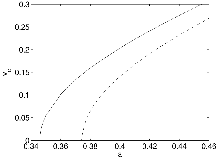
Figure 11: Critical velocity from the numerical stability analysis (solid) and the analytical approximation (25), (26) and (29) (dashed) for $q=0.9$ and $\varepsilon=1$.

References

- (1) J.D. Gunton, M.S. Miguel, P.S. Sahni, in Phase Transitions and Critical Phenomena, edited by C. Domb, J.L. Lebowitz (Academic Press, London, 1983), Vol. 8
- (2) A.J. Bray, Adv. Phys. 43, 357 (1994)
- (3) M.C. Cross, P.C. Hohenberg, Rev. Mod. Phys. 65, 851 (1993)
- (4) S. Walheim, E. Schaffer, J. Mlynek, U. Steiner, Science 283, 520 (1999)
- (5) M. Böltau, S. Walheim, J. Mlynek, G. Krausch, U. Steiner, Nature (London) 391, 877 (1998)
- (6) J. Vörös, T. Blättler, M. Textor, MRS Bull. 30, 202 (2005)
- (7) H. Sirringhaus, Adv. Mater. 17, 2411 (2005)
- (8) L. Berthier, Phys. Rev. E 63, 051503 (2001)
- (9) H. Tanaka, T. Sigehuzi, Phys. Rev. Lett. 75, 874 (1995)
- (10) A. Voit, A. Krekhov, W. Enge, L. Kramer, W. Köhler, Phys. Rev. Lett. 94, 214501 (2005)
- (11) A.P. Krekhov, L. Kramer, Phys. Rev. E 70, 061801 (2004)
- (12) R.E. Kelly, D. Pal, J. Fluid Mech. 86, 433 (1978)
- (13) M. Lowe, J.P. Gollub, T.C. Lubensky, Phys. Rev. Lett. 51, 786 (1983)
- (14) M. Lowe, B.S. Albert, J.P. Gollub, J. Fluid Mech. 173, 253 (1986)
- (15) P. Coullet, Phys. Rev. Lett. 56, 724 (1986)
- (16) P. Coullet, D. Repaux, Europhys. Lett. 3, 573 (1987)
- (17) P. Coullet, D. Walgraef, Europhys. Lett. 10, 525 (1989)
- (18) W. Zimmermann, A. Ogawa, S. Kai, K. Kawasaki, T. Kawakatsu, Europhys. Lett. 24, 217 (1993)
- (19) A. Ogawa, W. Zimmermann, K. Kawasaki, T. Kawakatsu, J. Phys. II (Paris) 6, 305 (1996)
- (20) Y. Hidaka, T. Fujimura, N.A. Mori, S. Kai, Mol. Cryst. & Liq. Cryst. 328, 565 (1999)
- (21) M. Henriot, J. Burguete, R. Ribotta, Phys. Rev. Lett. 91, 104501 (2003)
- (22) G. Hartung, F.H. Busse, I. Rehberg, Phys. Rev. Lett. 66, 2742 (1991)
- (23) W. Zimmermann, R. Schmitz, Phys. Rev. E 53, R1321 (1996)
- (24) R. Schmitz, W. Zimmermann, Phys. Rev. E 53, 5993 (1996)
- (25) H. Riecke, J.D. Crawford, E. Knobloch, Phys. Rev. Lett. 61, 1942 (1988)
- (26) D. Walgraef, Europhys. Lett. 7, 485 (1988)
- (27) I. Rehberg, S. Rasenat, J. Fineberg, M. de la Torre Juárez, V. Steinberg, Phys. Rev. Lett. 61, 2449 (1988)
- (28) A.L. Lin, M. Bertram, K. Martinez, H.L. Swinney, A. Ardelea, G.F. Carey, Phys. Rev. Lett. 84, 4240 (2000)
- (29) A.L. Lin, A. Hagberg, A. Ardelea, M. Bertram, H.L. Swinney, E. Meron, Phys. Rev. E 62, 3790 (2000)
- (30) A. Krekhov, Formation of regular structures in the process of phase separation, arXiv:0807.1708v1 [nlin.PS]
- (31) C. Utzny, W. Zimmermann, M. Bär, Europhys. Lett. 57, 113 (2002)
- (32) S. Rüdiger, D.G. Miguez, A.P. Munuzuri, F. Sagués, J. Casademunt, Phys. Rev. Lett. 90, 128301 (2003)
- (33) D.G. Miguez, E.M. Nicola, A.P. Munuzuri, J. Casademunt, F. Sagués, L. Kramer, Phys. Rev. Lett. 93, 048303 (2004)
- (34) S. Schuler, M. Hammele, W. Zimmermann, Eur. Phys. J B 42, 591 (2004)
- (35) S. Rüdiger, E.M. Nicola, J. Casademunt, L. Kramer, Phys. Rep 447, 73 (2007)
- (36) S. Rüdiger, J. Casademunt, L. Kramer, Phys. Rev. Lett. 99, 028302 (2007)
- (37) S. Wiegand, W. Köhler, in Thermal Nonequilibrium Phenomena in Fluid Mixtures, edited by W. Köhler, S. Wiegand (Springer, Heidelberg, 2002), p. 189
- (38) G. Wittko, W. Köhler, Phil. Mag. 83, 1973 (2003)
- (39) J.S. Langer, Ann. Phys. (N.Y.) 65, 53 (1971)