Low-momentum effective interaction in
the three-dimensional approach

Abstract

The formulation of the low-momentum effective interaction in the model space Lee-Suzuki and the renormalization group methods is implemented in the three-dimensional approach. In this approach the low-momentum effective interaction $V_{low\,k}$ has been formulated as a function of the magnitude of momentum vectors and the angle between them. As an application the spin-isospin independent Malfliet-Tjon potential has been used into the model space Lee-Suzuki method and it has been shown that the low-momentum effective interaction $V_{low\,k}$ reproduces the same two-body observables obtained by the bare potential $V_{NN}$.

I Introduction

One of the most fundamental and essential problems in the nuclear theory is the derivation of the effective interaction between the nucleons of nuclei. The conventional nuclear force models are given by the same one-pion exchange interaction in the long distance, but differ substantially in their treatment of the short distance. The fact that the different short distance structures reproduce the same observables for two-body problem indicates that low energy observables are insensitive to the details of the short distance dynamics. This insensitivity is a result of the separation of the high and low energy scales in the nuclear force, and implies that we can derive a low-momentum effective interaction.

During the past years, several methods have been developed to derive the energy independent low-momentum effective interaction such as the renormalization group (RG) and the model space techniques. These approaches are mainly based on a partial wave (PW) decomposition and the details have been given in references [1-11]. Bogner et al. have developed a low-momentum effective interaction which is quite successful in describing the two-nucleon system at low energy. This effective interaction is independent of the potential models as the cutoff is lowered to $\Lambda=2.1\,\,fm^{-1}$ Bogner-PR386 ; Bogner-PLB576 .

Recently the three-dimensional (3D) approach, which greatly simplifies the numerical calculations of few-body systems without performing the PW decomposition, is developed for few-body bound and scattering problems [12-27]. The motivation for developing this approach is introducing a direct solution of the integral equations avoiding the very involved angular momentum algebra occurring for the permutations, transformations and especially for the three-body forces. Conceptually the 3D formalism consider all partial wave channels automatically. Based on this non PW method the bound and scattering amplitudes are formulated as function of momentum vector variables, specially their magnitudes and the angle between them.

In this article our aim is to generate the low-momentum effective interaction directly in a 3D formalism, where as a simplification the spin and isospin degrees of freedom have been neglected in the first step. So the low-momentum effective interaction has been formulated for spinless identical particles as function of vector Jacobi momenta. Considering the spin and isospin degrees of freedom is a major additional task, which will increase more degrees of freedom into the states Bayegan-PRC77 . The formulation of the low-momentum effective interaction in a spin-isospin dependent 3D approach, based on helicity representation, is currently underway and it will be reported elsewhere Bayegan-p .

This article is organized as follows. In the section II the model space Lee-Suzuki method has been used to derive the energy independent model space effective interaction in the 3D representation. In addition a renormalization group decimation method has been performed in the 3D representation and a flow equation for the low-momentum effective interaction $V_{low\,k}$ has been obtained as a function of momentum vectors in the appendix A. The section III describes the details of the discussion and numerical calculations of the low-momentum effective interaction $V_{lowk}$ in the model space Lee-Suzuki method by using the spin-isospin independent toy Malfliet-Tjon potential. Finally a summary is given in the section IV and an outlook is provided.

II Model space Lee-Suzuki method for $V_{low\,k}$ in the 3D momentum representation

Several model space techniques such as the Bloch-Horowitz Bogner-PR386 ; Jennings-EL72 , the Unitary Transformation Epelbaum-PLB439 ; Fujii-PRC70 and the Lee-Suzuki [7-11] based on the restricted space, have been developed for the construction of the low-momentum effective interaction $V_{low\,k}$.

In this work the Lee-Suzuki formalism has been applied to the free space nucleon-nucleon problem in the 3D momentum representation and the low-momentum effective interaction $V_{low\,k}$ has been obtained as function of the momentum vectors. A momentum-space Hamiltonian for the full-space two-body problem has been considered as follows:

$$H(\textbf{k},\textbf{k}^{\prime})=H_{0}(\textbf{k})\delta(\textbf{k}-\textbf{k}^{\prime})+V_{NN}(\textbf{k},\textbf{k}^{\prime}),$$ (1)

where $H_{0}$ denotes the kinetic energy and $V_{NN}(\textbf{k},\textbf{k}^{\prime})$ is the bare two-body interaction. In the model space methods the projection operators onto the physically important low-energy model space, the $P$ space, and the high-energy complement, the $Q$ space, have been introduced as:

$$P = \int d^{3}k\,|\textbf{k}\rangle\langle\textbf{k}|,|\textbf{k}|\leq\Lambda,$$

$$Q = \int d^{3}k\,|\textbf{k}\rangle\langle\textbf{k}|,|\textbf{k}|>\Lambda,$$ (2)

where $\Lambda$ is a momentum cutoff which divides the Hilbert space into the low and high momentum states. These projections satisfy the relations:

$$P+Q = 1,$$

$$PQ = QP=0,$$

$$P^{2} = P,$$

$$Q^{2} = Q,$$ (3)

and they act on the full-space two-body problem states as:

$$P|\psi_{\textbf{k}}^{NN}\rangle = |\Psi_{\textbf{k}}^{NN}\rangle,$$

$$Q|\psi_{\textbf{k}}^{NN}\rangle = \omega|\Psi_{\textbf{k}}^{NN}\rangle,$$ (4)

where $|\psi_{\textbf{k}}^{NN}\rangle$ and $|\Psi_{\textbf{k}}^{NN}\rangle$ denote the states of the full and model spaces respectively. The $\omega$ is an operator which transforms the states of the $P$ space to the states of the $Q$ space. The key aspect of the Lee-Suzuki method is the determination of the $\omega$ operator defined by the following equation Jennings-EL72 :

$$Q|\psi_{\textbf{k}}^{NN}\rangle=Q\,\omega P|\psi_{\textbf{k}}^{NN}\rangle.$$ (5)

The Schrödinger equation for the full-space two-body problem by considering the equation (5) can be written as:

$$H|\psi_{\textbf{k}}^{NN}\rangle=H(P+Q)|\psi_{\textbf{k}}^{NN}\rangle=H(P+Q\,\omega P)|\psi_{\textbf{k}}^{NN}\rangle=E|\psi_{\textbf{k}}^{NN}\rangle.$$ (6)

By acting the $P$ operator on the left side of the last equation the full-space two-body problem has been reduced to the model space two-body problem of the following form:

$$PH(P+Q\,\omega P)|\psi_{\textbf{k}}^{NN}\rangle=(PH_{0}P+PVP+PVQ\,\omega P)|\psi_{\textbf{k}}^{NN}\rangle=EP|\psi_{\textbf{k}}^{NN}\rangle,$$ (7)

where we assumed that the $P$ and $Q$ operators commute with the $H_{0}$. Therefore the non-hermitian low-momentum effective potential in the model space that reproduces the model space components of the wave function from the full-space wave function can be written as [7-11]:

$$V_{low\,k}=PV(P+Q\omega P).$$ (8)

By using the integral form of the projection operators $P$ and $Q$, the low-momentum effective interaction $V_{low\,k}$ can be written in the 3D representation as:

$$V_{low\,k}(\textbf{k}^{\prime},\textbf{k})=V_{NN}(\textbf{k}^{\prime},\textbf{k})+\int_{\Lambda}^{\infty}dq\,q^{2}\int d\hat{\textbf{q}}\,\,V_{NN}(\textbf{k}^{\prime},\textbf{q})\,\omega(\textbf{q},\textbf{k}),$$ (9)

where q is the momentum vector in the complement model space $Q$. For an application we can choose the suitable coordinate system which the vector k is along the $z$ axis and the vector $\textbf{k}^{\prime}$ is in $x-z$ plane. So the equation (9) can be rewritten as:

$$V_{low\,k}(k^{\prime},k,x)=V_{NN}(k^{\prime},k,x)+\int_{\Lambda}^{\infty}dq\,q^{2}\int_{-1}^{1}dx^{\prime}\int_{0}^{2\pi}d\varphi\,\,V_{NN}(k^{\prime},q,y)\,\omega(q,k,x^{\prime}),$$

where:

$$x = \hat{\textbf{k}}\cdot\hat{\textbf{k}}^{\prime},$$

$$x^{\prime} = \hat{\textbf{k}}\cdot\hat{\textbf{q}},$$

$$y = \hat{\textbf{k}}^{\prime}\cdot\hat{\textbf{q}}=xx^{\prime}+\sqrt{1-x^{2}}\sqrt{1-x^{\prime 2}}\cos\varphi,$$

$$k = |\,\textbf{k}|,$$

$$k^{\prime} = |\,\textbf{k}^{\prime}|,$$

$$q = |\,\textbf{q}|.$$ (11)

To calculate the low-momentum effective potential $V_{low\,k}$ we need to determine $\omega$. To this aim by applying $\langle\textbf{q}|$ on the left side of equation (5) and using the integral form of projection operators $P$ and $Q$, this equation can be rewritten as follows:

$$\Psi_{\textbf{k}}^{NN}(\textbf{q})=\int_{0}^{\Lambda}dpp^{2}\int d\hat{\textbf{p}}\omega(\textbf{q},\textbf{p})\,\Psi_{\textbf{k}}^{NN}(\textbf{p}),$$ (12)

where p is the momentum vector in the model space. We use the completeness relation in the model space as:

$$\int_{0}^{\Lambda}dk\,k^{2}\int d\,\hat{\textbf{k}}\,\,\,\tilde{\Psi}_{\textbf{k}}^{NN}(\textbf{p}^{\prime})\Psi_{\textbf{k}}^{NN}(\textbf{p})=\delta(\textbf{p}^{\prime}-\textbf{p}).$$ (13)

The equation (12) after implementing equation (13) can be written as:

$$\omega(\textbf{q},\textbf{p})=\int_{0}^{\Lambda}dkk^{2}\int d\hat{\textbf{k}}\,\,\,\Psi_{\textbf{k}}^{NN}(\textbf{q})\tilde{\Psi}_{\textbf{k}}^{NN}(\textbf{p}),$$ (14)

where $\Psi_{\textbf{k}}^{NN}(\textbf{p})$ and $\Psi_{\textbf{k}}^{NN}(\textbf{q})$ are the wave function components of the $P$ and $Q$ spaces of the full-space respectively which in the form of the half-on-shell (HOS) two-body $T$ matrix are given by:

$$\Psi_{\textbf{k}}^{NN}(\textbf{q}) = \frac{T(\textbf{q},\textbf{k},k^{2})}{k^{2}-q^{2}},$$ (15)

$$\Psi_{\textbf{k}}^{NN}(\textbf{p}) = \delta(\textbf{p}-\textbf{k})+\frac{T(\textbf{p},\textbf{k},k^{2})}{k^{2}-p^{2}+i\varepsilon}$$ (16)

$$= \delta(\textbf{p}-\textbf{k})+\wp\frac{T(\textbf{p},\textbf{k},k^{2})}{k^{2}-p^{2}}-i\pi\,\delta(k^{2}-p^{2})\,T(\textbf{p},\textbf{k},k^{2}),$$

where $\wp$ denotes a principle value. The HOS two-body $T$ matrix can be obtained from the Lippmann-Schwinger equation in the 3D representation, which is given as Elster-FBS24 :

$$T(\textbf{k}^{\prime},\textbf{k},k^{2})=V_{NN}(\textbf{k}^{\prime},\textbf{k})+\int\emph{d}^{3}k^{\prime\prime}\frac{V_{NN}(\textbf{k}^{\prime},\textbf{k}^{\prime\prime})\,T(\textbf{k}^{\prime\prime},\textbf{k},k^{2})}{k^{2}-k^{\prime\prime 2}+i\varepsilon}.$$ (17)

In order to solve the equation (14) we have chosen suitable coordinate system which the vector q is along the $z$ axis and the vector p is in $x-z$ plane. Therefore the equation (14) can be rewritten as:

$$\omega(q,p,x)=\int_{0}^{\Lambda}dkk^{2}\int_{-1}^{1}dx^{\prime}\int_{0}^{2\pi}d\varphi\Psi_{k}^{NN}(q,x^{\prime})\tilde{\Psi}_{k}^{NN}(p,y),$$ (18)

where:

$$x = \hat{\textbf{q}}\cdot\hat{\textbf{p}},$$

$$x^{\prime} = \hat{\textbf{q}}\cdot\hat{\textbf{k}},$$

$$y = \hat{\textbf{k}}\cdot\hat{\textbf{p}}=xx^{\prime}+\sqrt{1-x^{2}}\sqrt{1-x^{\prime 2}}\cos\varphi,$$

$$k = |\,\textbf{k}|,$$

$$p = |\,\textbf{p}|,$$

$$q = |\,\textbf{q}|.$$ (19)

We should mention that the Lee-Suzuki method reproduces the HOS two-body T matrix the same as the RG method, therefore the solution of this approach has been proven to be equivalent to the solution of the RG equation Bogner-nt ; Bogner-PLB500 . In appendix (A) we derive a renormalization group decimation method in the 3D representation and we obtain a flow equation for the low-momentum effective interaction $V_{low\,k}$ for future applications.

III Discussion and Numerical results

In our calculations we employ the spin-isospin independent Malfliet-Tjon potential. This force is a superposition of a short-range repulsive and long-range attractive Yukawa interactions. It is given as Malfliet-NPA127 :

$$V_{NN}(\textbf{k}^{\prime},\textbf{k})=\frac{1}{2\pi^{2}}\,(\frac{V_{R}}{(\textbf{k}^{\prime}-\textbf{k})^{2}+\mu_{R}^{2}}-\frac{V_{A}}{(\textbf{k}^{\prime}-\textbf{k})^{2}+\mu_{A}^{2}}).$$ (20)

With the strengths and the masses of the meson exchange as follow: $V_{R}=7.291,V_{A}=3.177,\mu_{R}=613.7MeV,\mu_{A}=305.9MeV$. This potential supports one bound state at $E=-2.23MeV$. With this interaction we first implement the LU factorization into equation (13) to calculate $\tilde{\Psi}_{k}^{NN}(p^{\prime},x^{\prime},\varphi^{\prime})$ as an inverse of the wave function $\Psi_{k}^{NN}(p,x,\varphi)$ in the model space. Then by solving the equation (18) we calculate $\omega(q,p,x)$ and finally we input the $\omega$ operator into equation (II) to obtain the low-momentum effective interaction $V_{low\,k}(p^{\prime},p,x)$.

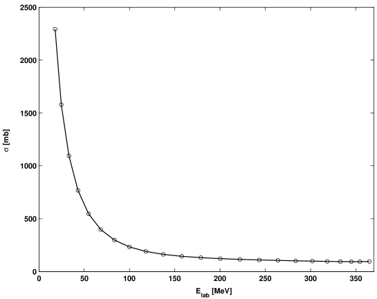
Figure 1: The total two-body cross section from the low-momentum effective potential (circles) and the bare potential (solid line) as a function of kinetic energy in the lab frame.

Figure 2: The two-body $S$-wave phase shift from the low-momentum effective potential (circles) and the bare potential (solid line) as a function of kinetic energy in the lab frame.

The dependence on the continuous momentum and the angle variables is replaced in the numerical treatment by a dependence on the certain discrete values. To this aim we use the Gaussian quadrature grid points to discrete the momentum and the angle variables. In our calculations we choose forty grid points for the momentum variables in the $P$ space, i.e. the interval $[0,\Lambda]$, and thirty grid points for the momentum variables in the $Q$ space, i.e. the interval $[\Lambda,\infty)$. Also twenty and fourteen grid points for the spherical and the polar angle variables have been used respectively. The integration interval for the $P$ and $Q$ spaces are covered by two different linear and tangential mappings the Gauss-Legendre points $x$ from the interval (-1,+1) via:

$$p = \frac{\Lambda}{2}(1+x),$$

$$q = b\,tan\left(\frac{\pi}{4}(1+x)\right)+\Lambda\,\,,\,b=5\,fm^{-1}.$$ (21)

to the intervals $[0,\Lambda]$ and $[\Lambda,\infty)$ respectively. As we mentioned in the introduction we have used the value of $2.1\,fm^{-1}$ for the cutoff $\Lambda$ in our calculations. The solution of the integral equation (17) requires a one-dimensional interpolation on $T$. We use the cubic hermitian splines of ref. 59 for its accuracy and high computational speed. It can be useful to mention that in the numerical calculations we use the Lapack library 60 , for solving a system of linear equations in the calculation of the two-body $T$ matrix.

Figure 3: (a) The comparison of the low-momentum effective potential $V_{low\,k}(p.p,x)$ (solid lines) with the bare potential $V_{NN}(p,p,x)$ (dashed lines) and (b) differences between them.

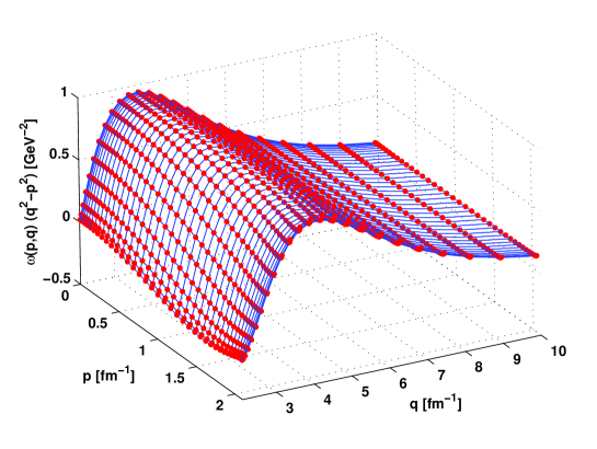
Figure 4: The comparison of $\omega(q,p)(q^{2}-p^{2})$ operator for the $S$-wave calculated in the PW approach (dotes) and in the 3D approach (solid lines).

Figure 5: The comparison of the low-momentum effective potential $V_{{}_{low\,k}}(p^{\prime},p)$ for the $S$-wave calculated in the PW approach (dotes) and in the 3D approach (solid lines).

We have shown in figure 1 that the calculated total two-body cross section for the $V_{low\,k}(p^{\prime},p,x)$ and the $V_{NN}(p^{\prime},p,x)$ match perfectly well. Also we have calculated the $S$-wave phase shift for $V_{low\,k}(p^{\prime},p,x)$ and it has been compared with the obtained result with the bare potential $V_{NN}(p^{\prime},p,x)$ in figure 2. For calculation of the phase shift we have used the relation between the PW and 3D representations of the on-shell $T$ matrix as follow:

$$T_{l}(p,p,p^{2})=2\pi\int_{-1}^{1}dx\,\,\,T(p,p,x,p^{2})\,P_{l}(x).$$ (22)

As we expect the results are in good agreement with the high accuracy. In figure (3a) we have compared the calculated low-momentum effective potential $V_{low\,k}(p,p,x)$ with the bare potential $V_{NN}(p,p,x)$, also In figure (3b) the difference between them is shown as a function of the momentum variable $p$ and the angle variable $x$. This comparison demonstrates that the difference between the two potentials is approximately constant except for the momentum values close to the cutoff, where the differences vary for different angle values. Conceptually when we integrate on the angles we can produce the same results as PW approach.

As a test of our calculations we can compare the obtained results for the low-momentum effective potential and the $\omega$ operator in both 3D and PW approaches. In the first step we directly calculate the $\omega$ operator and the low-momentum effective potential in PW approach. In the second step we obtain a certain PW projection of the $\omega$ operator and the low-momentum effective potential from their corresponding 3D representation by the following relations:

$$V^{l}_{low\,k}(p^{\prime},p) = 2\pi\int_{-1}^{1}dx\,\,\,V_{low\,k}(p^{\prime},p,x)\,P_{l}(x),$$

$$\omega_{l}(q,p) = 2\pi\int_{-1}^{1}dx\,\,\,\omega(q,p,x)\,P_{l}(x).$$ (23)

The obtained results for the $S$-wave projection of the $\omega$ operator and the low-momentum effective potential in both of 3D and PW approaches are given in figures (4) and (5) respectively. The agreement between the two approaches is quiet satisfactory.

IV Summary and Outlook

In this article the 3D formulation of the Lee-Suzuki and the RG methods have been presented. The low-momentum effective interaction $V_{low\,k}$ has been derived as a function of the magnitude of momenta and the angle between them without using the partial wave decomposition. The calculated two-body observables from the low-momentum effective interaction and the bare interaction have been shown. In addition a comparison of calculated $V_{low\,k}$ from the PW and the 3D representation have been demonstrated as a test for our calculations.

The advantage of our formulation in the 3D representation in comparison with the PW representation is that we have calculated the low-momentum effective interaction by considering all partial waves automatically.

For the future investigations the low-momentum effective interaction can be formulated by considering the spin and isospin degrees of freedom in a realistic 3D approach. This formulation based on the momentum helicity basis has been done and the calculation of the realistic low-momentum effective interaction with Bonn-B, AV18 and Chiral potentials is currently underway. Considering the obtained 3D low-momentum effective interaction in the few-body bound and scattering calculations is another major task to be done.

Appendix A RG method for $V_{low\,k}$ in the 3D momentum representation

For the two-body problem, the RG method derives the low-momentum effective potential $V_{low\,k}$ by integrating out the model dependent high momentum component of the different models of bare potentials $V_{NN}$ by demanding that the low-momentum observables calculated from $V_{NN}$ must be reproduced by $V_{low\,k}$ with the same accuracy. We follow basically the same procedure which is used by Bogner et al. in derivation of the RG flow equation Bogner-nt . However instead of using the PW representation, we have implemented the treatment of the RG in the 3D representation. We start with a RG treatment of the scattering problem in the 3D representation. The HOS two-body $T$ matrix in 3D representation by applying an arbitrary potential model $V_{NN}$ to the scattering problem is given by the Lippmann-Schwinger equation $(\hbar=m_{N}=1)$ Elster-FBS24 :

$$T(\textbf{k}^{\prime},\textbf{k},k^{2})=V_{NN}(\textbf{k}^{\prime},\textbf{k})+\wp\int_{0}^{\infty}\emph{d}p\,p^{2}\int\emph{d}\,\hat{\textbf{p}}\frac{V_{NN}(\textbf{k}^{\prime},\textbf{p})\,T(\textbf{p},\textbf{k},k^{2})}{k^{2}-p^{2}},$$ (24)

where $\wp$ denotes a principle value integration. Corresponding to equation (7) we can define a restricted version of the equation (24) by imposing a cutoff $\Lambda$ and replacing the bare potential $V_{NN}$ by a low-momentum effective potential $V_{low\,k}$ as:

$$T_{low\,k}(\textbf{k}^{\prime},\textbf{k},k^{2})=V_{low\,k}(\textbf{k}^{\prime},\textbf{k})+\wp\int_{0}^{\Lambda}\emph{d}p\,p^{2}\int\emph{d}\,\hat{\textbf{p}}\frac{V_{low\,k}(\textbf{k}^{\prime},\textbf{p})\,T_{low\,k}(\textbf{p},\textbf{k},k^{2})}{k^{2}-p^{2}}.$$

We demand that the calculated low-momentum HOS two-body T matrices from equations (24) and (A) are identical, i.e. $T(\textbf{k}^{\prime},\textbf{k},k^{2})=T_{low\,k}(\textbf{k}^{\prime},\textbf{k},k^{2})$ for $|\textbf{k}^{\prime}|,\,|\textbf{k}|\leq\Lambda$. This condition ensures that the $V_{low\,k}$ gives the same low-momentum two-body observables as obtained by the bare potential $V_{NN}$. Imposing the cutoff independence of the low-momentum HOS two-body $T$ matrix, i.e. $dT(\textbf{k}^{\prime},\textbf{k},k^{2})/d\Lambda=0$ in equation (A), ensures that the low-momentum observables will be independent of the scale $\Lambda$ and will generate energy-independent potential $V_{low\,k}$, therefore we obtain:

$$\int_{0}^{\Lambda}\emph{d}\,p\,p^{2}\int\emph{d}\,\hat{\textbf{p}}\frac{dV_{lowk}(\textbf{k}^{\prime},\textbf{p})}{d\Lambda}\,\chi_{\textbf{k}}(\textbf{p})=\int d\hat{\mathbf{p}}\frac{V_{lowk}(\textbf{k}^{\prime},\Lambda\hat{\mathbf{p}})\,T(\Lambda\hat{\mathbf{p}},\textbf{k},k^{2})}{1-(k/\Lambda)^{2}},$$ (26)

where we have used the standing wave scattering states of the effective theory $|\chi_{\textbf{k}}\rangle$, which can be written as:

$$|\chi_{\textbf{k}}\rangle=|\textbf{k}\rangle+\wp\int_{0}^{\Lambda}\emph{d}p\,p^{2}\int\emph{d}\,\hat{\textbf{p}}\frac{T(\textbf{p},\textbf{k},k^{2})}{k^{2}-p^{2}}\,\,\,|\textbf{p}\rangle.$$ (27)

By using the completeness relation of the scattering states in the model space and considering $T(\Lambda\hat{\mathbf{p}},\textbf{k},k^{2})=\langle\Lambda\hat{\mathbf{p}}|V_{lowk}|\chi_{\textbf{k}}\rangle$, we have obtained:

$$\frac{d}{d\Lambda}\langle\,\textbf{k}^{\prime}|V_{low\,k}|\textbf{p}^{\prime}\rangle = \Lambda^{2}\int d\hat{\mathbf{p}}\,\,\langle\,\textbf{k}^{\prime}|V_{low\,k}|\Lambda\hat{\mathbf{p}}\rangle$$ (28)

$$\times\int_{0}^{\Lambda}dk\,k^{2}\int d\,\hat{\textbf{k}}\frac{\langle\Lambda\hat{\mathbf{p}}|V_{low\,k}|\chi_{\textbf{k}}\rangle}{\Lambda^{2}-k^{2}}\langle\tilde{\chi}_{\textbf{k}}|\textbf{p}^{\prime}\rangle$$

$$= \Lambda^{2}\int d\hat{\mathbf{p}}\langle\,\textbf{k}^{\prime}|V_{low\,k}|\Lambda\hat{\mathbf{p}}\rangle\int_{0}^{\Lambda}dp^{\prime\prime}p^{\prime\prime 2}\int d\,\hat{\textbf{p}}^{\prime\prime}\langle\Lambda\hat{\mathbf{p}}|V_{low\,k}|\textbf{p}^{\prime\prime}\rangle$$

$$\times\int_{0}^{\Lambda}dk\,k^{2}\int d\,\hat{\textbf{k}}\frac{\langle\textbf{p}^{\prime\prime}|\chi_{\textbf{k}}|\rangle\langle\tilde{\chi}_{\textbf{k}}|\textbf{p}^{\prime}\rangle}{\Lambda^{2}-k^{2}}$$

$$= \Lambda^{2}\int d\,\hat{\mathbf{p}}\langle\textbf{k}^{\prime}|V_{low\,k}|\Lambda\hat{\mathbf{p}}\rangle$$

$$\times\int_{0}^{\Lambda}dp^{\prime\prime}p^{\prime\prime 2}\int d\,\hat{\textbf{p}}^{\prime\prime}\langle\Lambda\hat{\mathbf{p}}|V_{low\,k}|\textbf{p}^{\prime\prime}\rangle G(\textbf{p}^{\prime\prime},\textbf{p}^{\prime},\Lambda^{2}),$$

where $\langle\tilde{\chi}_{\textbf{k}}|$ is the bi-orthogonal complement in completeness relation in the model space which satisfies $\langle\tilde{\chi}_{\textbf{k}^{\prime}}|\chi_{\textbf{k}}\rangle=\delta(\textbf{k}^{\prime}-\textbf{k})$ and $G$ denotes the interacting Green’s function in the model space. With writing the $G$ in terms of the two-body $T$ matrix we obtain the RG equation in the 3D momentum representation as:

$$\frac{d}{d\Lambda}V_{low\,k}(\textbf{k}^{\prime},\textbf{k})=\int d\hat{\mathbf{p}}\frac{V_{low\,k}(\textbf{k}^{\prime},\Lambda\hat{\mathbf{p}})\,T(\Lambda\hat{\mathbf{p}},\textbf{k},\Lambda^{2})}{1-(k/\Lambda)^{2}}.$$ (29)

For numerical calculations we can choose the suitable coordinate system where the vector $\textbf{k}^{\prime}$ is along the $z$ axis and the vector k is in $x-z$ plane. By this consideration we can rewrite the above equation as:

$$\frac{d}{d\Lambda}V_{low\,k}(k^{\prime},k,x)=\int_{-1}^{1}dx^{\prime}\int_{0}^{2\pi}d\varphi\frac{V_{low\,k}(k^{\prime},\Lambda,x^{\prime})\,T(\Lambda,k,y,\Lambda^{2})}{1-(k/\Lambda)^{2}},$$ (30)

where:

$$x = \hat{\textbf{k}}^{\prime}\cdot\hat{\textbf{k}},$$

$$x^{\prime} = \hat{\mathbf{k}}^{\prime}\cdot\hat{\textbf{p}},$$

$$y = \hat{\textbf{k}}\cdot\hat{\mathbf{p}}=xx^{\prime}+\sqrt{1-x^{2}}\sqrt{1-x^{\prime 2}}\cos\varphi,$$

$$k = |\,\textbf{k}|,$$

$$k^{\prime} = |\,\textbf{k}^{\prime}|.$$ (31)

We introduce:

$$\hat{T}(k^{\prime},k,x^{\prime},x)=\int_{0}^{2\pi}d\varphi\,T(k^{\prime},k,x^{\prime}x+\sqrt{1-x^{\prime 2}}\sqrt{1-x^{2}}\cos\varphi).$$ (32)

And finally the RG equation in the 3D representation can be obtained:

$$\frac{d}{d\Lambda}V_{low\,k}(k^{\prime},k,x)=\int_{-1}^{1}dx^{\prime}\frac{V_{low\,k}(k^{\prime},\Lambda,x^{\prime})\,\hat{T}(\Lambda,k,x^{\prime},x,\Lambda^{2})}{1-(k/\Lambda)^{2}}.$$ (33)

The low-momentum effective interaction $V_{low\,k}(k^{\prime},k,x)$ can be calculated by numerically integrating the RG equation on the Gaussian momentum and angle grid points. Similar to the PW representation of this equation, $V_{NN}(k^{\prime},k,x)$ can be used as a large-cutoff initial condition to calculate $V_{low\,k}(k^{\prime},k,x)$ numerically.

References

• (1) S. K. Bogner, T. T. S. Kuo and A. Schwenk, Phys. Rep. 386 (2003) 1.
• (2) S. K. Bogner, T. T. S. Kuo, A. Schwenk, D.R. Entem and R. Machleit, Phys. Let. B576 (2003) 265.
• (3) E. Epelbaum, W. Glöckle, U.G Meißner, Phys. Let. B439 (1998) 1.
• (4) S. K. Bogner, A. Schwenk, T. T. S. Kuo and G. E. Brown, nucl-th/0111042.
• (5) S. Fujii, E. Epelbaum, H. Kamada, R. Okamoto, K. Suzuki and W. Glockle, Phys. Rev. C70 (2004) 024003.
• (6) M. C. Birse, J. A. McGovern and K. G. Richardson, Phys. Lett. B464 (1999) 169.
• (7) K. Suzuki, Prog. Theor. Phys. 68 (1982) 246.
• (8) S. Y. Lee and K. Suzuki, Phys. Lett. B91 (1980) 173.
• (9) K. Suzuki and R. Okamoto, Prog. Theor. Phys. 92 (1994) 1045.
• (10) K. Suzuki and S.Y. Lee, Prog. Theor. Phys. 64 (1980) 2091.
• (11) K. Suzuki and R. Okamotp, Prog. Theor. Phys. 70 (1983) 439.
• (12) Ch. Elster, J. H. Thomas and W. Glöckle, Few Body Systems 24 (1998) 55.
• (13) Ch. Elster, W. Schadow, A. Nogga and W. Glöckle, Few Body Systems 27 (1999) 83.
• (14) W. Schadow, Ch. Elster and W. Glöckle, Few Body Systems 28 (2000) 15.
• (15) I. Fachruddin, Ch. Elster and W. Glöckle, Phys. Rev. C 62 (2000) 044002.
• (16) I. Fachruddin, Ch. Elster and W. Glöckle, Phys. Rev. C 63 (2001) 054003.
• (17) H. Liu, Ch. Elster and W. Glöckle, Few Body Systems 33 (2003) 241.
• (18) I. Fachruddin, Ch. Elster and W. Glöckle, Mod. Phys. Lett. A18 (2003) 452.
• (19) I. Fachruddin, Ch. Elster and W. Glöckle, Phys. Rev. C68 (2003) 054003.
• (20) I. Fachruddin, W. Glöckle, Ch. Elster and A. Nogga, Phys. Rev. C69 (2004) 064002.
• (21) H. Liu, Ch. Elster and W. Glöckle, Phys. Rev. C72 (2005) 054003.
• (22) T. Lin, Ch. Elster, W. N. Polyzou, and W. Glöckle, Phys. Let. B660 (2008) 345.
• (23) M. R. Hadizadeh and S. Bayegan, Few Body Systems 40 (2007) 171.
• (24) M. R. Hadizadeh and S. Bayegan, Eur. Phys. J. A36 (2008) 201.
• (25) S. Bayegan, M. R. Hadizadeh and M. Harzchi, Phys. Rev. C77 (2008) 064005.
• (26) S. Bayegan, M. R. Hadizadeh and M. Harzchi, to appear in Few Body Systems, arXiv:0711.4036.
• (27) S. Bayegan, M. R. Hadizadeh and W. Glöckle, Submitted to Prog. of Theor. Phys. arXiv:0806.1520.
• (28) S. Bayegan, M. Harzchi and M. R. Hadizadeh, in preparation.
• (29) B. K. Jennings, Europhys. Lett 72 (2005) 211.
• (30) S. K. Bogner and T.T.S. Kuo, Phys. Lett. B500 (2001) 279.
• (31) R. A. Malfliet and J. A. Tjon, Nucl. Phys. A127 (1969) 161.
• (32) D. Hüber, H. Witala, A. Nogga, W. Glöeckle and H. Kamada, Few Body Systems 22 (1997) 107.
• (33) the routines called ZGESV from http://netlib.org/lapack/double/