Twenty-five years of multifractals in fully developed turbulence: a tribute to Giovanni Paladin

Abstract

The paper On the multifractal nature of fully developed turbulence and chaotic systems, by R. Benzi et al. published in this journal in 1984 ( vol 17, page 3521) has been a starting point of many investigations on the different faces of selfsimilarity and intermittency in turbulent phenomena.
Since then, the multifractal model has become a useful tool for the study of small scale turbulence, in particular for detailed predictions of different Eulerian and Lagrangian statistical properties.
In the occasion of the 50-th birthday of our unforgettable friend and colleague Giovanni Paladin (1958-1996), we review here the basic concepts and some applications of the multifractal model for turbulence.

I Introduction

The idea of the multifractal approach to fully developed turbulence has been introduced by Giorgio Parisi and Uriel Frisch during the Summer School Turbulence and predictability of geophysical fluid dynamics held in Varenna in June 1983 PF85 . One of us (A.V.) had the chance to participate to that school and then to coauthor, with R. Benzi, G. Parisi and G.Paladin, the paper published in this journal where the word multifractal appeared for the first time BPPV84 .

From a technical point of view the idea of the multifractal is basically contained in the large deviation theory Ellis99 ; Varadhan03 which is an important chapter of the probability theory. However the introduction of the multifractal description in the 1980’s had an important role in statistical physics, chaos and disordered systems. In particular to clarify in a rather net way that the usual idea, coming from the critical phenomena, that just few scaling exponents are relevant, is wrong, while an infinite set of exponents is necessary for a complete characterization of the scaling features.
As pioneering works which anticipated some aspects of the the multifractal approach to turbulence we can cite the lognormal theory of Kolmogorov K62 , the contributions of Novikov and Stewart NS64 and Mandelbrot M74 .

This paper has no pretense to be a survey of the many applications of the multifractal description in chaos, disordered systems and natural phenomena; for general reviews on these aspects see BS95 ; BP97 ; Meakin98 . For a more mathematically oriented treatment see Harte01 . Our aim is a discussion on the the use of the multifractal methods in the study of the scaling features of fully developed turbulence.

The paper is organized as follows. Section II is devoted to the introduction of the multifractal model of turbulence and its connections with the $f(\alpha)$ vs $\alpha$ formalism introduced by Halsey et al. HJKPS86 , and the large deviations theory Ellis99 ; Varadhan03 . In Section III we discuss the implication of multifractality on Eulerian features, namely the statistical properties of the velocity gradients and the existence of an intermediate dissipative range. Section IV is devoted to the implications of the multifractal nature of turbulence on Lagrangian statistics. In Section 5 we present the Lagrangian acceleration statistics. Section 6 treats the relative dispersion, in particular we discuss the multifractal generalization of the classical Richardson theory. Section 7 is devoted to the multifractal analysis of the dispersion in two-dimensional convection.

II From Kolmogorov to multifractals

Let us consider the Navier-Stokes equations for an incompressible fluid:

$${\partial{\bf v}\over\partial t}+({\bf v}\cdot\nabla){\bf v}=-{1\over\rho}\nabla p+\nu\Delta{\bf v}+{\bf F}\,,\qquad\nabla\cdot{\bf v}=0\,\,.$$ (1)

Because of the nonlinear structure of the equation, an analytical treatment is a formidable task. For instance in the $3D$ case a theorem for the existence of global solution for arbitrary $\nu$ is still missing.

For a perfect fluid (i.e. $\nu=0$) and in absence of external forces (${\bf F}=0$), the evolution of the velocity field is given by the Euler equation, which conserves the kinetic energy for smooth solutions. In such a case, introducing an ultraviolet cutoff $K_{max}$ on the wave numbers, it is possible to build up an equilibrium statistical mechanics simply following the standard approach used for the Hamiltonian statistical mechanics. On the other hand, because of the so called dissipative anomaly F95 ; BJPV98 , in $3D$ the limit $\nu\to 0$ is singular and cannot be interchanged with $K_{max}\to\infty$, therefore the statistical mechanics of an inviscid fluid has a rather limited relevance for the Navier-Stokes equations at very high Reynolds numbers ($Re=VL/\nu$, where $V$ and $L$ are the typical speed and length of the system, respectively).

In addition, mainly as a consequence of the non-Gaussian statistics, even a systematic statistical approach, e.g. in term of closure approximations, is very difficult F95 ; BJPV98 .

In the fully developed turbulence (FDT) limit, i.e. $\nu\to 0$, and in the presence of forcing at large scale, one has a non equilibrium statistical steady state, with an inertial range of scales, where neither energy pumping nor dissipation acts, which shows strong departures from the equipartition F95 ; BJPV98 . A simple and elegant explanation of the main statistical features of FDT is due to Kolmogorov MY75 : in a nutshell, it is assumed the existence of a range of scales where the energy – injected at the scale $L$ – flows down (with a cascade process, as remarked by Richardson R22 ) to the dissipative scale $\ell_{D}\sim LRe^{-3/4}$, where it is dissipated by molecular viscosity. Since, practically, neither injection nor dissipation takes place in the inertial range, the only relevant quantity is the average energy transfer rate $\bar{\varepsilon}$. Dimensional counting imposes the power law dependence for the second order structure function (SF)

$$S_{2}(\ell)=\langle\delta v_{\ell}^{2}\rangle=\langle\left(v(x+\ell)-v(x)\right)^{2}\rangle\propto\bar{\varepsilon}^{2/3}\ell^{2/3}\,,$$ (2)

where, for the sake of simplicity, we ignore the vectorial nature of the velocity field. The scaling law (2) is equivalent to a power spectrum $E(k)\propto\bar{\varepsilon}^{2/3}k^{-5/3}$ in good agreement with the experimental observations. The original Kolmogorov theory (often indicated as K41) assumes self-similarity of the turbulent flow. As a consequence, the scaling behavior of higher order structure functions

$$S_{p}(\ell)=\langle|v(x+\ell)-v(x)|^{p}\rangle\sim\ell^{\zeta_{p}}$$ (3)

is described by a single scaling exponent: $\zeta_{p}=p/3$.

II.1 The multifractal model

The Navier-Stokes equations are formally invariant under the scaling transformation:

$${\bf x}\to\lambda\,{\bf x}\,\,\,\,,{\bf v}\to\lambda^{h}\,{\bf v}\,\,\,\,,t\to\lambda^{1-h}\,t\,\,\,,\,\,\,\nu\to\lambda^{h+1}\nu\,\,,$$

with $\lambda>0$ (indeed the Reynolds number $VL/\nu$ is invariant under the above transformations).

The exponent $h$ cannot be determined with only symmetry considerations, nevertheless there is a rather natural candidate: $h=1/3$. Such a value of the exponent is suggested by the dimensional argument of the K41 and also, and more rigorously, by the so-called “4/5 law”, an exact relation derived by Kolmogorov from the Navier–Stokes equations K41 ; F95 , which, under the assumption of stationarity, homogeneity and isotropy, states

$$\langle\delta v^{3}_{||}(\ell)\rangle=-{4\over 5}\bar{\varepsilon}\ell\,,$$ (4)

where $\delta v_{||}(\ell)$ is the longitudinal velocity difference between two points at distance $\ell$.

We can say that the K41 theory corresponds to a global invariance with $h=1/3$ and therefore $\zeta_{p}=p/3$. This result is in disagreement with several experimental investigations AGHA84 ; F95 which have shown deviations of the scaling exponents from $p/3$. This phenomenon, which goes under the name of intermittency F95 , is a consequence of the breakdown of self–similarity and implies that the scaling exponents cannot be determined on a simple dimensional basis.

A simple way to modify the K41 consists in assuming that the energy dissipation is uniformly distributed on homogeneous fractal with dimension $D_{F}<3$. This implies $\delta v_{\ell}({\bf x})\sim\ell^{h}$ with $h=(D_{F}-2)/3$ for ${\bf x}$ on the fractal and $\delta v_{\ell}({\bf x})$ non singular otherwise. This assumption (called absolute curdling or $\beta$- model) gives:

$$\zeta_{p}={{D_{F}-2}\over 3}p+(3-D_{F})\,.$$ (5)

Such a prediction, with $D_{F}\simeq 2.83$ , is in fair agreement with the experimental data for small values of $p$, but higher order scaling exponents give a clear indication of a non linear behavior in $p$.

The multifractal model of turbulence PF85 ; PV87 ; F95 assumes that the velocity has a local scale-invariance, i.e. there is not a unique scaling exponent $h$ such that $\delta v_{\ell}\sim\ell^{h}$, but a continuous spectrum of exponents, each of which belonging to a given fractal set. In other words, in the inertial range one has

$$\delta v_{\ell}({\bf x})\sim\ell^{h}\,,$$ (6)

if ${\bf x}\in S_{h}$, and $S_{h}$ is a fractal set with dimension $D(h)$ and $h\in$ ($h_{min}$, $h_{max}$). The probability to observe a given scaling exponent $h$ at the scale $\ell$ is $P_{\ell}(h)\sim\ell^{3-D(h)}$ and therefore one has

$$S_{p}(\ell)=\langle|\delta v_{\ell}|^{p}\rangle\sim\int_{h_{min}}^{h_{max}}\ell^{hp}\ell^{3-D(h)}{\rm d}h\sim\ell^{\zeta_{p}}\,.$$ (7)

For $\ell\ll 1$, a steepest descent estimation gives

$$\zeta_{p}=\min_{h}\left\{hp+3-D(h)\right\}=h^{*}p+3-D(h^{*})$$ (8)

where $h^{*}=h^{*}(p)$ is the solution of the equation $D^{\prime}(h^{*}(p))=p$. The Kolmogorov “4/5” law (4) imposes $\zeta_{3}=1$ which implies that

$$D(h)\leq 3h+2\,,$$ (9)

with the equality realized by $h^{*}(3)$. The Kolmogorov similarity theory corresponds to the case of only one singularity exponent $h=1/3$ with $D(h=1/3)=3$.

Of course the computation of $D(h)$, or equivalently $\zeta_{p}$, from the NSE is not at present an attainable goal. A first step is a phenomenological approach using multiplicative processes. Let us briefly remind the so called random $\beta$- model BPPV84 . This model describes the energy cascade in real space looking at eddies of size $\ell_{n}=2^{-n}L$, with $L$ the length at which the energy is injected. At the $n$- th step of the cascade a mother eddy of size $\ell_{n}$ splits into daughter eddies of size $\ell_{n+1}$, and the daughter eddies cover a fraction $\beta_{j}$ ($0<\beta_{j}<1$) of the mother volume. As a consequence of the fact that the energy transfer is constant throughout the cascade one has for the velocity differences $v_{n}=\delta v_{\ell_{n}}$ on scale $\ell_{n}$ is non negligible only on a fraction of volume $\prod_{j}\beta_{j}$, and it is given by

$$v_{n}=v_{0}\ell_{n}^{1/3}\prod_{j=1}^{n}\beta_{j}^{-1/3}$$ (10)

where the $\beta_{j}$’s are independent, identically distributed random variables. Phenomenological arguments suggest: $\beta_{j}=1$ with probability $x$ and $\beta_{j}=B=2^{-(1-3h_{min})}$ with probability $1-x$ The above multiplicative process generates a two-scale Cantor set, which is a rather common structure in chaotic systems. The scaling exponents are:

$$\zeta_{p}={p\over 3}-\ln_{2}[x+(1-x)B^{1-p/3}]\,\,$$ (11)

corresponding to

$$D(h)=3+\bigl{(}3h-1\bigr{)}\Bigl{[}1+\ln_{2}\Bigl{(}{{1-3h}\over{1-x}}\Bigr{)}\Bigr{]}+3h\ln_{2}\left({x\over 3h}\right)\,.$$ (12)

The two limit cases are $x=1$, i.e. the K41, and $x=0$ which is the $\beta$- model with $D_{F}=2+3h_{min}$. Using $x=7/8$, $h_{min}=0$ (i.e. $B=1/2$) one has a good fit for the $\zeta_{p}$ of the experimental data at high Reynolds numbers.

Figure 1: Structure function scaling exponents $\zeta_{p}$ plotted vs $p$. Circles and triangles correspond to the data of Anselmet at al. AGHA84 . The solid line corresponds to Kolmogorov scaling $p/3$; the dashed line is the random beta model prediction (11) with $B=1/2$ and $x=7/8$; the dotted line is the She-Leveque prediction (13) with $\beta=2/3$.

Of course it is not so astonishing to find a model to fit the experimental data. Indeed, there are now many phenomenological models for $D(h)$ which provide scaling exponents in agreement with experimental data. A popular one is the so-called She-Leveque model SheLeveque94 which is reproduced by the multifractal model with

$$D(h)=1+{2\beta-3h-1\over\ln\beta}\left[1-\ln\left({2\beta-1-3h\over 2\ln\beta}\right)\right]$$

and gives for the scaling exponents

$$\zeta_{p}={2\beta-1\over 3}p+2(1-\beta^{p/3})$$ (13)

which are close to the experimental data for $\beta=2/3$. Another important model, which was introduced by Kolmogorov himself without reference to the multifractal model, is the log-normal model which will be discussed in Section II.2.

The relevance, and the success, of the multifractal approach is in the possibility to predict, and test, nontrivial statistical features, e.g. the pdf of the velocity gradient, the existence of an intermediate dissipative range and precise scaling for Lagrangian quantities. Once $D(h)$ is obtained by a fit of the experimental data, e.g. from the $\zeta_{p}$, then all the predictions obtained in the multifractal model framework must be verified without additional free parameters.

II.2 Relation between the original multifractal model and the $f(\alpha)$ vs $\alpha$

The multifractal model for the FDT previously discussed is linked to the so called $f(\alpha)$ vs $\alpha$ description of the singular measures (e.g. in chaotic attractors) HJKPS86 ; BJPV98 ; AFLV92 . In order to show this connection let us recall the Kolmogorov revised theory K62 (called K62) stating that the velocity increments $\delta v_{\ell}$ scales as $(\epsilon_{\ell}\ell)^{1/3}$ where $\epsilon_{\ell}$ is the energy dissipation space-averaged over a cube of edge $\ell$. Let us introduce the measure $\mu({\bf x})=\epsilon({\bf x})/{\bar{\epsilon}}$, a partition of non overlapping cells of size $\ell$ and the coarse graining probability

$$P_{i}(\ell)=\int_{\Lambda_{\ell}({\bf x})}d\mu({\bf y})$$

where $\Lambda_{l}({\bf x}_{i})$ is a cube of edge $\ell$ centered in ${\bf x}_{i}$, of course $\epsilon_{\ell}\sim\ell^{-3}P(\ell)$. Denoting with $\alpha$ the scaling exponent of $P_{\ell}$ and with $f(\alpha)$ the fractal dimension of the subfractal with scaling exponent $\alpha$, we can introduce the Renyi dimensions $d_{p}$:

$$\sum_{i}P_{i}(\ell)^{p}\sim\ell^{(p-1)d_{p}}$$

where the sum is over the non empty boxes. A simple computation gives

$$(p-1)d_{p}=\min_{\alpha}[p\alpha-f(\alpha)]\,\,.$$

Noting that $<\epsilon_{\ell}^{p}>=\ell^{3}\sum\epsilon_{\ell}^{p}$ we have

$$<\epsilon_{\ell}^{p}>\sim\ell^{(p-1)(d_{p}-3)}$$

therefore one has the correspondence

$$h\leftrightarrow{{\alpha-2}\over 3}\,\,\,,\,\,\,D(h)\leftrightarrow f(\alpha)\,\,\,,\,\,\,\zeta_{p}={p\over 3}+\bigl{(}{p\over 3}-1\bigr{)}\bigl{(}d_{p\over 3}-3\bigr{)}\,\,.$$

Of course the result $\zeta_{3}=1$, once assumed $\delta v\sim(\epsilon_{\ell}\ell)^{1/3}$, holds for any $f(\alpha)$. Let us note that the lognormal theory K62 where

$$\zeta_{p}={p\over 3}+{\mu\over 18}p(3-p)$$

is a special case of the multifractal model, where there are not restriction on the values of $h$ and $D(h)$ is a parabola with a maximum at $D_{F}=3$:

$$D(h)=-{9\over 2\mu}h^{2}+{3\over 2}(2+\mu)h-{4-20\mu+\mu^{2}\over 8\mu}$$

and the parameter $\mu$ is determined by the fluctuation of $\ln\epsilon_{\ell}$.

II.3 A technical remark on multifractality

To obtain the scaling behavior of $S_{p}(\ell)\sim(\ell/L)^{\zeta_{p}}$ given by (7) with $\zeta_{p}$ obtained from (8), one has to assume that the exponent $ph+3-D(h)$ has a minimum, $\zeta_{p}$, which is a function of $h$, and that such an exponent behaves quadratically with $h$ in the vicinity of the minimum. This is the basic assumption to apply the Laplace’s method of steepest descent BO99 . The point we would like to recall here is that, for small separations, $\ell$, it is true that $S_{p}(\ell)\sim(\ell/L)^{\zeta_{p}}$ but with a logarithmic prefactor:

$$S_{p}(\ell)\sim\left[-\ln\left(\frac{\ell}{L}\right)\right]^{-1/2}\left(\frac{\ell}{L}\right)^{\zeta_{p}}$$ (14)

Such a prefactor is usually not considered in the naive application of Laplace method leading to (7). The presence of such logarithmic correction, if present, would clearly invalidate the $4/5$-th law (4), one of the very few exact results in fully developed turbulence.
The question on whether such logarithmic correction is likely has quantitatively been addressed by Frisch et al. FMMY05 . There, exploiting the refined large-deviations theory, the Authors were able to explain in which way the logarithmic contribution cancels out thus giving rise to a prediction fully compatible with the naive (a priory unjustified) procedure to extract the scaling behavior (7). The key point is that the leading order large deviation result for the probability $P_{\ell}(h)$ to be within a distance $\ell$ of the set carrying singularities of scaling exponent between $h$ and $h+dh$,

$$P_{\ell}(h)\sim\left(\frac{\ell}{L}\right)^{3-D(h)}\;,$$ (15)

must be generalized to take into account next subleading order. In doing so, as a result one obtains FMMY05

$$P_{\ell}(h)\sim\left(\frac{\ell}{L}\right)^{3-D(h)}\left[-\ln\frac{\ell}{L}\right]^{1/2},$$ (16)

which contains subleading logarithmic correction. It is worth observing that despite the multiplicative character of the logarithmic correction one speaks of “subleading correction”. This is justified by the fact that the correct statement of the large-deviations leading-order result involves the logarithm of the probability divided by the logarithm of the scale. The correction is then a subleading additive term.
Once the expression (16) is plugged in the integral

$$S_{p}(\ell)\sim\int dhP_{\ell}(h)\left(\frac{\ell}{L}\right)^{ph}$$ (17)

and the saddle point estimation is carried out according to BO99 , logarithms disappear and the expected $4/5$-th law emerges.
It is worth mentioning that the presence of a square root of a logarithm correction in the multifractal probability density had already been proposed by MS89 on the basis of a normalization requirement. In that paper, the Authors observed that without such a correction the singularity spectrum $f(\alpha)$ comes out wrong; they also pointed out that a similar correction has been proposed by vdWS88 in connection with the measurement of generalized Renyi dimensions.

III Implications of multifractality on Eulerian features

At first we note that a consequence of presence of the intermittency the Kolmogorov scale does not take a unique value. The local dissipative scale $\ell_{D}$ is determined by imposing the effective Reynolds number to be of order unity:

$$Re(\ell_{D})={\delta v_{D}\ell_{D}\over\nu}\sim 1\,,$$ (18)

therefore the dependence of $\ell_{D}$ on $h$ is thus

$$\ell_{D}(h)\sim LRe^{-{1\over 1+h}}$$ (19)

where $Re=Re(L)$ is the large scale Reynolds number PV_PRA87 .

In this section we will show that the fluctuations of the dissipative scale, due to the intermittency in the turbulent cascade, is relevant of the statistical features of the velocity differences and velocity gradient, and in addition it implies the existence of an intermediate region between the inertial and dissipative range FV91 .

III.1 The Pdf of the velocity differences and velocity gradient

Let us denote by $s$ the longitudinal velocity gradient. Such a quantity can immediately be expressed in terms of the singularity exponents $h$ as

$$|s|\sim\frac{\delta v_{\ell_{D}}}{\ell_{D}}=v_{0}\ell_{D}^{h-1}=v_{0}^{\frac{2}{1+h}}\nu^{\frac{h-1}{h+1}}$$ (20)

where we used the fact that $\delta v_{\ell}\sim v_{0}l^{h}$ from (6) and we have exploited (19). From (20) we realize that we can easily express the probability density function (PDF) of $s$ (for a fixed $h$), $P_{h}(s)$, in terms of the PDF, $\Pi(V_{0})$, of the large-scale velocity differences $V_{0}$, with $v_{0}\equiv|V_{0}|$. The latter PDF is indeed known to be accurately described by the Gaussian distribution FS91 . The link between the two PDFs is given by the standard relation:

$$P_{h}(s)=\Pi(V_{0})\left|\frac{dV_{0}}{ds}\right|$$ (21)

from which one immediately gets:

$$P_{h}(s)\sim\frac{\nu}{|s|}^{\frac{1-h}{2}}e^{-\frac{\nu^{1-h}|s|^{1+h}}{2\langle V_{0}^{2}\rangle}}.$$ (22)

The K41 theory and the $\beta$ model correspond to $h=1/3$ and $h=(D_{F}-2)/3$, respectively. In both cases, a stretched exponential form for the PDF is predicted with an exponent, $1+h$, larger than one. Experimental data (see e.g. CGH90 ; VM91 ) are not consistent with such a prediction being actually compatible with a stretched exponent whose value is smaller than one.
The multifractal description has thus to be exploited to capture those experimental evidences. To do that we recall the expression (10) for the random $\beta$ model

$$v_{n}=v_{0}\ell_{n}^{1/3}\prod_{j=1}^{n}\beta_{j}^{-1/3}$$ (23)

from which the probability distribution of the velocity increments $v_{n}$ reads:

$$P(v_{n})=\int\Pi(V_{0})dV_{0}\int\delta(v_{n}-v_{0}l_{n}^{1/3}\prod_{i=1}^{n}\beta_{i}^{-1/3})\prod_{j=1}^{n}\beta_{i}\mu(\beta_{i})d\beta_{i}.$$ (24)

Here $\mu(\beta_{i})$ is the probability density of the $\beta_{i}$’s assumed to be of the form:

$$\mu(\beta_{i})=x\delta(\beta_{i}-1)+(1-x)\delta(\beta_{i}-B)$$ (25)

with $B=2^{-(1-3h_{min})}$.
Since the $\beta_{i}$’s are identically distributed, the above integral becomes:

$$P(v_{n})=\sum_{K=0}^{n}{n\choose K}x^{n-K}(1-x)^{K}B^{4K/3}l_{n}^{-1/3}e^{-CB^{2K/3}l_{n}^{-2/3}v_{n}^{2}}$$ (26)

with $C\equiv(2\langle V_{0}^{2}\rangle)^{-1}$. It is easy to see BBPVV91 the passage of the above PDF from a Gaussian form at large scales (small $n$) to an exponential-like form at small scales (large $n$).
To obtain the gradient PDF from (26) it is sufficient to stop the sum at $n=N$ such that $v_{N}l_{N}/\nu=1$. This is equivalent to say

$$l_{N}^{2}=2^{-2N}\sim\frac{\nu}{s}\qquad\mbox{or}\qquad N=\frac{\ln\frac{s}{\nu}}{2\ln 2}.$$ (27)

By noting that $B^{2N}=(\nu/s)^{1-3h_{min}}$ the resulting gradient PDF reads:

$$P(s)\sim\sum_{K=0}^{N}{N\choose K}x^{N-K}(1-x)^{K}\left(\frac{\nu}{|s|}\right)^{(1+2q)/3}e^{-C\nu^{(2+q)/3}|s|^{(4-q)/3}}$$ (28)

where $q\equiv K(1-3h_{min})/N$. The K41 prediction corresponds to considering only the term $K=0$ with $x=1$.
We already discussed that $x=7/8$ and $h_{min}=0$ provides a good fit for the scaling exponents $\zeta_{p}$ of the structure functions in the limit of high Reynolds numbers. The same parameters give a PDF behavior in good agreement with available experimental data (see BBPVV91 and Figure 2).

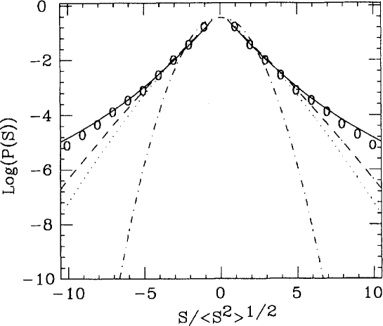
Figure 2: Log-linear plot of the PDF of velocity gradients $s$ rescaled with the rms value. Points represent experimental data from VM91 , solid line is the multifractal prediction with the random beta model, dotted and dashed lines represent the K41 and beta model results respectively.

III.2 Intermediate dissipative range

Let us now show, that as consequence of the fluctuations of the dissipative scale one has the existence of an intermediate region (the Intermediate Dissipative Range, IDR) between the inertial and dissipative range FV91 . The presence of fluctuations of $\ell_{D}$, see (19), modifies the evaluation of the structure functions (7): for a given $\ell$, the saddle point evaluation remains unchanged if, for the selected exponent $h^{*}(p)$, one has $\ell_{D}(h^{*}(p))<\ell$. If, on the contrary, the selected exponent is such that $\ell_{D}(h^{*}(p))>\ell$ the saddle point evaluation is not consistent, because at scale $\ell$ the power–law scaling (6) is no longer valid. In this intermediate dissipation range the integral in (7) is dominated by the smallest acceptable scaling exponent $h(\ell)$ given by inverting (19), and the structure function of order $p$ a pseudo–algebraic behavior, i.e. a power law with exponent $ph(\ell)+3-D(h(\ell))$ which depends on the scale $\ell$. Taking into account the fluctuations of the dissipative range FV91 , one has for the structure functions

$$S_{p}(\ell)\sim\left\{\begin{array}[]{lll}\ell^{\zeta_{p}}&\mbox{if}&\ell_{D}(h^{*}(p))<\ell\\ \ell^{h(\ell)p+3-D(h(\ell))}&\mbox{if}&\ell_{D}(h_{min})<\ell<\ell_{D}(h^{*}(p))\,.\end{array}\right.$$ (29)

A simple calculation FV91 ; F95 shows that it is possible to find a universal description valid both in the inertial and in the intermediate dissipative ranges. Let us discuss this point for the energy spectrum $E(k)$. Introducing the rescaled variables

$$F(\theta)={\ln E(k)\over\ln Re}\qquad{\mbox{and}}\qquad\theta={\ln k\over\ln Re}$$ (30)

one obtains the following behavior

$$F(\theta)=\left\{\begin{array}[]{lll}-(1+\zeta_{2})\theta&\mbox{for}&\theta<{1\over 1+h^{*}(2)}\\ -2-2\theta+\theta D(\theta^{-1}-1)&\mbox{for}&{1\over 1+h^{*}(2)}<\theta<{1\over 1+h_{min}}\end{array}\right.$$ (31)

The prediction of the multifractal model is that $\ln E(k)/\ln Re$ is an universal function of $\ln k/\ln Re$. This is in contrast with the usual scaling hypothesis according which $\ln E(k)$ should be a universal function of $\ln(k/k_{D})$). The multifractal universality has been tested by collapsing energy spectra obtained from turbulent flow in a wide range of $Re$ GC91 , see also BCVV99 .

III.3 Exit times for turbulent signals and the IDR

In the following we will discuss a method alternative to the study of the structure functions which allows for a deeper understanding of the IDR.

Basically in typical experiments one is forced to analyze one-dimensional string of data $v(t)$, e.g. the output of hot-wire anemometer, and the Taylor Frozen-Turbulence Hypothesis is used to bridge measurements in space with measurements in time. As a function of time increment, $\tau$, structure functions assume the form: $S_{p}(\tau)=<\!\!\left[(v(t+\tau)-v(t)\right]^{p}\!\!>$. In the inertial range, $\tau_{D}\ll\tau\ll T_{0}$ (where $T_{0}=L_{0}/V_{0}$, and the dissipative time, $\tau_{D}=\ell_{D}/V_{0}$) the structure functions develop an anomalous scaling behavior: $S_{p}(\tau)\sim\tau^{\zeta_{p}}$, where $\tau\sim\ell/V_{0}$.

The main idea, which can be applied both to experimental and synthetic data, is to take a time sequence $v(t)$, and to analyze the statistical properties of the exit times from a set of defined velocity-thresholds. More precisely, given a reference initial time $t_{0}$ with velocity $v(t_{0})$, we define $\tau(\delta v)$ as the first time necessary to have an absolute variation equal to $\delta v$ in the velocity data, i.e. $|v(t_{0})-v(t_{0}+\tau(\delta v))|=\delta v$. By scanning the whole time series we recover the probability density functions of $\tau(\delta v)$ at varying $\delta v$ from the typical large scale values down to the smallest dissipative values. Positive moments of $\tau(\delta v)$ are dominated by events with a smooth velocity field, i.e. laminar bursts in the turbulent cascade. Let us define the Inverse Structure Functions (Inverse-SF) as BCVV99 ; J99 :

$$\Sigma_{p}(\delta v)\equiv<\!\!\tau^{p}(\delta v)\!\!>\,.$$ (32)

It is necessary to perform weighted average over the time-statistics in a weighted way. This is due to the fact that by looking at the exit-time statistics we are not sampling the time-series uniformly, i.e. the higher the value of $\tau(\delta v)$ is, the longer it remains detectable in the time series.
It is possible to show BCFV02 that the sequential time average of any observable, ${\cal A}$, based on exit-time statistics, $\langle{\cal A}\rangle_{e}$, is connected to the uniformly-in-time multifractal average by the relation:

$$\langle A\rangle=\frac{\langle A\tau\rangle_{e}}{\langle\tau\rangle_{e}}\,.$$ (33)

For ${\cal A}=\tau^{p}(\delta v)$ the above relations becomes:

$$\langle\tau^{p}(\delta v)\rangle=\frac{\langle\tau^{p+1}\rangle_{e}}{\langle\tau\rangle_{e}}\,.$$ (34)

According to the multifractal description we assume that, for velocity thresholds corresponding to inertial range values of the velocity differences the following dimensional relation is valid:

$$\delta_{\tau}v\sim\tau^{h}\;\;\rightarrow\;\;\tau(\delta v)\sim\delta v^{1/h}\,,$$

and the probability to observe a value $\tau$ for the exit time is given by inverting the multifractal probability, i.e. $P(\tau\sim\delta v^{1/h})\sim\delta v^{[3-D(h)]/h}$. With this ansatz in the inertial range one has:

$$\Sigma_{p}(\delta v)\sim\int_{h_{\mathrm{min}}}^{h_{\mathrm{max}}}dh\;\delta v^{[p+3-D(h)]/h}\sim\delta v^{\chi_{p}}$$ (35)

where with the Laplace method one obtains:

$$\chi_{p}=\min_{h}\left\{[p+3-D(h)]/h\right\}\,.$$ (36)

Let us now consider the IDR properties.
For each $p$, the saddle point evaluation selects a particular $h=h_{s}(p)$ where the minimum is reached. Let us also remark that from (35) we have an estimate for the minimum value assumed by the velocity in the inertial range given a certain singularity $h$: $v_{m}(h)=\delta_{\tau_{d}(h)}v\sim\nu^{h/(1+h)}$. Therefore, the smallest velocity value at which the scaling (35) still holds depends on both $\nu$ and $h$. Namely, $\delta v_{m}(p)\sim\nu^{h_{s}(p)/1+h_{s}(p)}$. The most important consequence is that for $\delta v<\delta v_{m}(p)$ the integral (35) is not any more dominated by the saddle point value but by the maximum $h$ value still dynamically alive at that velocity difference, $1/h(\delta v)=-1-\log(\nu)/\log(\delta v)$. This leads for $\delta v<\delta v_{m}(p)$ to a pseudo-algebraic law:

$$\Sigma_{p}(\delta v)\sim\delta v^{{\textstyle[p+3-D(h(\delta v))]/h(\delta v)}}\,.$$ (37)

The presence of this $p$-dependent velocity range, intermediate between the inertial range, $\Sigma_{p}(\delta v)\sim\delta v^{\chi_{p}}$, and the dissipative scaling, $\Sigma_{p}(\delta v)\sim\delta v^{p}$, is the IDR signature.

Figure 3: Inverse Structure Functions $\Sigma_{1}(\delta v)$. The straight lines shows the dissipative range behavior (dashed) $\Sigma_{1}(\delta v)\sim\delta v$, and the inertial range non intermittent behavior (dotted) $\Sigma_{1}(\delta v)\sim(\delta v)^{3}$. The inset shows the direct structure function $S_{1}(\tau)$ with superimposed the intermittent slope $\zeta_{1}=0.39$.

In Figure 3 we show $\Sigma_{1}(\delta v)$ evaluated on a string of high-Reynolds number experimental data as a function of the available range of velocity thresholds $\delta v$. This data set has been measured in a wind tunnel at $Re_{\lambda}\sim 2000$. One can see that the scaling is very poor. On the other hand, (inset of Figure 3), the scaling behavior of the direct structure functions $<\!|\delta v(\tau)|\!>\sim\tau^{\zeta_{1}}$ is quite clear in a wide range of scales. This is a clear evidence of IDR’s contamination into the whole range of available velocity values for the Inverse-SF cases.

Let us now go back to the statistical properties of the IDR. In order to study this question we have smoothed the stochastic synthetic field, $v(t)$ (see Appendix) by performing a running-time average over a time-window, $\delta T$. Then we compare Inverse-SF obtained for different Reynolds numbers, i.e. for different dissipative cut-off: $Re\sim\delta T^{-4/3}$.
The expression (37) predicts the possibility to obtain a data collapse of all curves with different Reynolds numbers by rescaling the Inverse-SF as follows FV91 ; JPV91 :

$$-{\ln(\Sigma_{p}(\delta v))}/{\ln(\delta T/\delta T_{0})}\;\;vs.\;\;-{\ln(\delta v/U)}/{\ln(\delta T/\delta T_{0})}\,,$$ (38)

where $U$ and $\delta T_{0}$ are adjustable dimensional parameters.

Figure 4: Data collapse of the Inverse-SF, $\Sigma_{1}(\delta v)$, obtained by the rescaling (38) for the smoothed synthetic signals (with time windows: $\delta T=4.8\cdot 10^{-4}\,,\;3\cdot 10^{-5}\,,\;2\cdot 10^{-6}$) and the experimental data ($EXP$). The two straight lines have the dissipative (solid line) and the inertial range (dashed) slope.

Figure 4 shows the rescaling (38) of the Inverse-SF, $\Sigma_{1}(\delta v)$, both for the synthetic field at different Reynolds numbers and for the experimental signals. As it is possible to see, the data-collapse is very good. This is a clear evidence that the poor scaling range observed in Figure 4 for the experimental signal can be explained as the signature of the IDR.

IV The relation between Eulerian and Lagrangian statistics

A problem of great interest concerns the study of the spatial and temporal structure of the so-called passive fields, indicating by this term quantities transported by the flow without affecting the velocity field. The paradigmatic equation for the evolution of a passive scalar field $\theta({\bf x},t)$ advected by a velocity field ${\bf v}({\bf x},t)$ is ShraimanSiggia00

$$\partial_{t}\theta+\nabla\cdot({\bf v}\,\theta)=\chi\,\nabla^{2}\theta$$ (39)

where $\chi$ is the molecular diffusion coefficient.

The problem (39) can be studied through two equivalent approaches, both due to Euler Lamb45 . The first, referred to as “Eulerian”, deals at any time with the field $\theta$ in the space domain covered by the fluid; the second considers the time evolution of trajectories of each fluid particle and is called “Lagrangian”.

The motion of a fluid particle is determined by the differential equation

$$\frac{d{\bf x}}{dt}={\bf v}({\bf x},t)$$ (40)

which also describes the motion of test particles, for example a powder embedded in the fluid, provided that the particles are neutral and small enough not to perturb the velocity field, although large enough not to perform a Brownian motion. Particles of this type are commonly used for flow visualization in fluid mechanics experiments T88 . We remark that the complete equation for the motion of a material particle in a fluid when density and volume effects are taken into account can be rather complicated MR83 ; BBCLT06a .

The Lagrangian equation of motion (40) formally represents a dynamical system in the phase space of physical coordinates. By very general considerations, it is now well established that even in regular velocity field the motion of fluid particles can be very irregular H66 ; A84 . In this case initially nearby trajectories diverge exponentially and one speaks of Lagrangian chaos or chaotic advection. In general, chaotic behaviors can arise in two-dimensional flow only for time dependent velocity fields, while it can be present even for stationary velocity fields in three dimensions.

If $\chi=0$, it is easy to realize that (39) is equivalent to (40). Indeed, we can write

$$\theta({\bf x},t)=\theta({T}^{-t}{\bf x},0)$$ (41)

where ${T}$ is the formal evolution operator of (40): ${\bf x}(t)={T}^{t}{\bf x}(0)$.

Taking into account the molecular diffusion $\chi$, (39) is the Fokker-Planck equation of the Langevin equation Chandrasekhar43

$${d{\bf x}\over dt}={\bf v}({\bf x},t)+{\eta}(t)$$ (42)

where ${\eta}$ is a Gaussian process with zero mean and variance

$$\left\langle{\eta_{i}(t)\,\eta_{j}(t^{\prime})}\right\rangle=2\chi\delta_{ij}\,\delta(t-t^{\prime}).$$ (43)

The dynamical system (40) becomes conservative in the phase space in the case of an incompressible velocity field for which

$$\nabla\cdot{\bf v}=0$$ (44)

In two dimensions, ${\bf x}=(x_{1},x_{2})$, the constraint (44) is automatically satisfied by introducing the stream function $\psi({\bf x},t)$

$$v_{1}={\partial\psi\over\partial x_{2}},\qquad v_{2}=-\,{\partial\psi\over\partial x_{1}}$$ (45)

and the evolution equation becomes

$${{dx_{1}}\over{dt}}={\partial\psi\over\partial x_{2}},\qquad{{dx_{2}}\over{dt}}=-\,{\partial\psi\over\partial x_{1}}.$$ (46)

i.e. formally a Hamiltonian system with the Hamiltonian given by the stream function $\psi$.

The presence of Lagrangian chaos in regular flows is a remarkable example of the fact that, in general, it is very difficult to relate Lagrangian and Eulerian statistics. For example, from very complicated trajectories of buoys one cannot infer the time-dependent circulation of the sea. In the following Sections we will see that in the case of fully developed turbulence, the disordered nature of the flow makes this connection partially possible at a statistical level.

The equation of motion (40) shows that the trajectory of a single particle is not Galilean invariant, i.e. invariant with respect to the addition of a mean velocity. The most general Galilean invariant statistics, which is ruled by small scale velocity fluctuation, is given by multi-particle, multi-time correlations for which we could expect universal features. In the following we will consider separately the two most studied statistics: single-particle two-time velocity differences and two-particle single-time relative dispersion.

IV.1 Single particle statistics: multifractal description of Lagrangian velocity differences

The simplest Galilean invariant Lagrangian quantity is the single particle velocity increment $\delta{\bf v}(t)={\bf v}(t_{0}+t)-{\bf v}(t_{0})$, where ${\bf v}(t)={\bf v}({\bf x}(t),t)$ denotes the Lagrangian velocity of the particle at ${\bf x}(t)$ and the independence on $t_{0}$ is a consequence of the stationarity of the flow. Dimensional analysis in fully developed turbulence predicts MY75 ; TL72

$$\langle\delta v_{i}(t)\delta v_{j}(t)\rangle=C_{0}\bar{\varepsilon}t\delta_{ij}$$ (47)

where $\bar{\varepsilon}$ is the mean energy dissipation and $C_{0}$ is a numerical constant. The remarkable coincidence that the variance of $\delta{\bf v}(t)$ grows linearly with time is the physical basis on which stochastic models of particle dispersion are based. It is important to recall that the “diffusive” nature of (47) is purely incidental: it is a direct consequence of Kolmogorov scaling in the inertial range of turbulence and is not directly related to a diffusive process (i.e. there is no decorrelation justifying the applicability of central limit theorem).

Let us recall briefly the argument leading to the scaling in (47). We can think at the velocity $v(t)$ advecting the Lagrangian trajectory as the superposition of the different velocity contributions coming from turbulent eddies (which also move with the same velocity of the Lagrangian trajectory). After a time $t$ the components associated to the smaller (and faster) eddies, below a certain scale $\ell$ are decorrelated and thus at the leading order one has $\delta v(t)\simeq\delta v(\ell)$. Within Kolmogorov scaling, the velocity fluctuation at scale $\ell$ is given by $\delta v(\ell)\sim V_{0}(\ell/L)^{1/3}$ where $V_{0}$ represents the typical velocity at the largest scale $L$. The correlation time of $\delta v(\ell)$ scales as $\tau(\ell)\sim\tau_{0}(\ell/L)^{2/3}$ and thus one obtains the scaling in (47) with $\varepsilon=V_{0}^{2}/\tau_{0}$.

Equation (47) can be generalized to higher order moments with the introduction of a set of temporal scaling exponents $\xi_{p}$

$$\langle\delta v(t)^{p}\rangle\sim V_{0}^{p}(t/\tau_{0})^{\xi_{p}}$$ (48)

The dimensional estimation sketched above gives the prediction $\xi_{p}=p/2$ but one may expect corrections to the dimensional scaling in the presence of intermittency.

A generalization of the above results which takes into account intermittency corrections can be easily developed by using the multifractal model Borgas93 ; BDM02 . The dimensional argument is repeated for the local scaling exponent $h$, giving $\delta v(t)\sim V_{0}(t/\tau_{0})^{h/(1-h)}$. Integrating over the $h$ distribution one ends with

$$\langle\delta v(t)^{p}\rangle\sim V_{0}^{p}\int dh\left({t\over\tau_{0}}\right)^{[ph-D(h)+3]/(1-h)}\,.$$ (49)

where $D(h)$ is the Eulerian fractal dimension (i.e. related to the Eulerian structure function scaling exponents by $\zeta(q)=\min_{h}[qh-D(h)+3]$). In the limit $t/\tau_{0}\to 0$, the integral can be estimated by a steepest descent argument giving the prediction

$$\xi_{p}=\min_{h}\left[{ph-D(h)+3\over 1-h}\right]$$ (50)

The standard inequality in the multifractal model $D(h)\leq 3h+2$ implies for (50) that even in the presence of intermittency $\xi_{2}=1$. Physically, this is a consequence of the fact that energy dissipation is raised to the first power, in (47).

Experimental results MMMP01 have shown that even at large Reynolds number the scaling (47) is not clearly observed. Therefore the dimensionless constant $C_{0}$ is known with large uncertainty, if compared with the Kolmogorov constant.

Intermittency in Lagrangian velocity differences is evident by looking at the pdf of $\delta v(t)$ at different time lags, as shown in Fig. 5. For large time delays the pdf are close to Gaussian while decreasing $t$ they develop larger and larger tails, implying the breakdown of self-similarity.

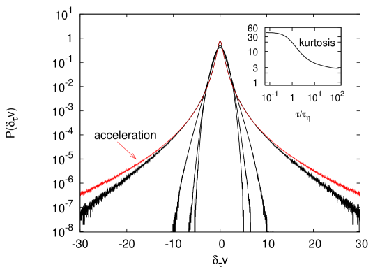
Figure 5: Probability density functions of velocity increments for a numerical simulation at $R_{\lambda}=284$. Curves refer to time increments $t=(97,24,6,0.7)\tau_{D}$ from inside to outside (and to the acceleration). In the inset kurtosis $\langle\delta v(t)^{4}\rangle/\langle\delta v(t)^{2}\rangle^{2}$ as a function of time delay is shown. Figure from BBCLT06 .

Higher order Lagrangian structure functions are shown in Fig. 6 for a set of direct numerical simulations at $R_{\lambda}=284$ BBCLT05 ; BBCLT06 . Despite the apparent scaling observed in the log-log plot, the computation of local slopes does not give a definite value of scaling exponents. Assuming $\xi_{2}=1$ as predicted by (50), one can measure the relative scaling exponent $\xi_{p}/\xi_{2}$ by using the so-called extended self-similarity procedure BCTBMS93 . As shown by the inset of Fig. 6, we observe a well defined scaling in the range of separations $10\tau_{D}\leq\tau\leq 50\tau_{D}$. The values of the relative exponents estimated with this method, $\xi_{4}/\xi_{2}=1.7\pm 0.05$, $\xi_{5}/\xi_{2}=2.0\pm 0.05$, $\xi_{6}/\xi_{2}=2.2\pm 0.07$, are in good agreement with those predicted by the multifractal model (50).

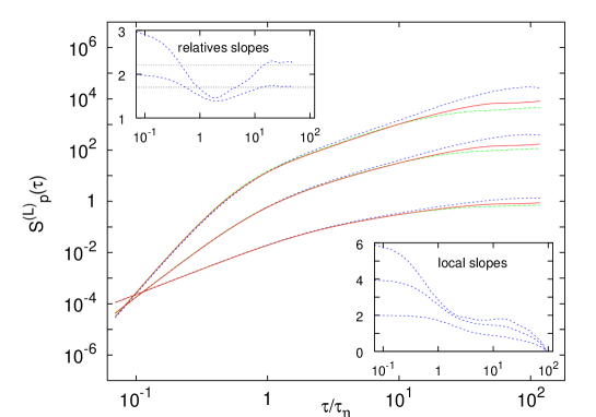
Figure 6: Log-log plot of Lagrangian structure functions of order $2$, $4$ and $6$ (bottom to top) for the three components of the velocity obtained from DNS at $R_{\lambda}=284$. Small differences between the components are observed at large delays as a consequence of small anisotropies at large scales. In the insets the local slopes (bottom right) and relative slopes (top left) are shown for the $x$-component. Relative slopes are defined as $dS_{p}(t)/dS_{2}(t)$ for $p=4,6$. The horizontal lines represent the multifractal prediction. Figure from BBCLT06 .

The multifractal prediction (50) has been checked also in simplified Lagrangian model based on the shell model of turbulence BDM02 .

V Lagrangian acceleration statistics

Acceleration in fully developed turbulence is an extremely intermittent quantity which display fluctuations up to $80$ times its root mean square LVCAB01 . These extreme events generate very large tails in the pdf of acceleration which are therefore expected to be very far from Gaussian.

We remark that even within non-intermittent Kolmogorov scaling, acceleration pdf is expected to be non-Gaussian. Indeed acceleration can be estimated from velocity fluctuations at the Kolmogorov scale as

$$a={\delta v(\tau_{D})\over\tau_{D}}$$ (51)

where $\tau_{D}=\eta/\delta v(\eta)$ and the Kolmogorov scale $\eta$ is given by the condition $\eta\delta v(\eta)/\nu=1$. By assuming the scaling $\delta v(\ell)\simeq V_{0}(\ell/L)^{h}$ (with $h=1/3$ for Kolmogorov scaling) one obtains

$${\eta\over L}\sim\left({V_{0}L\over\nu}\right)^{-{1\over 1+h}}$$ (52)

and therefore

$$a={V_{0}^{2}\over L}\left({V_{0}L\over\nu}\right)^{1-2h\over 1+h}$$ (53)

Assuming a Gaussian distribution for large scale velocity fluctuations $V_{0}$ (which is, as already observed, consistent with many experimental and numerical observations), and taking $h=1/3$, one obtains for the pdf of $a$ a stretched exponential tail $p(a)\sim\exp(-Ca^{8/9})$.

In the presence of intermittency the above argument has to be modified by taking into account the fluctuations of scaling exponent. In the recent years, several models have been proposed for describing turbulent acceleration statistics, on the basis of different physical ingredients. In the following we want to show that the multifractal model of turbulence, when extended to describe fluctuation at the dissipative scale, is able to predict the pdf of acceleration observed in simulations and experiments with high accuracy BBCDLT04 . Moreover, as in the case of Lagrangian structure functions, the model does not require the introduction of new parameters, a part the set of Eulerian scaling exponents. In this sense, multifractal model become a predictive model for Lagrangian statistics.

The introduction of intermittency in the above argument is simply obtained by weighting (53) with both the distribution of $V_{0}$ (still assumed Gaussian, as intermittency is not expected to affect large scale statistics) and the distribution of scaling exponent $h$ which can be rewritten as

$$p(h)\sim\left({\eta\over L}\right)^{3-D(h)}\sim\left({V_{0}L\over\nu}\right)^{D(h)-3\over 1+h}$$ (54)

The final prediction, when written for the dimensionless acceleration $\tilde{a}=a/\langle a^{2}\rangle^{1/2}$, becomes BBCDLT04

$$p(\tilde{a})\sim\int_{h}\tilde{a}^{[h-5+D(h)]/3}R_{\lambda}^{y(h)}\exp\left(-{1\over 2}\tilde{a}^{2(1+h)/3}R_{\lambda}^{z(h)}\right)dh$$ (55)

where $y(h)=\chi(h-5+D(h))/6+2(2D(h)+2h-7)/3$ and $z(h)=\chi(1+h)/3+4(2h-1)/3$. The coefficient $\chi$ is the scaling exponent for the Reynolds dependence of the acceleration variance, $\langle a^{2}\rangle\sim R_{\lambda}^{\chi}$, given by $\chi=\sup_{h}\left(2(D(h)-4h-1)/(1+h)\right)$. For the non-intermittent Kolmogorov scaling ($h=1/3$ and $D(1/3)=3$) one obtains $\chi=1$ and (55) recovers the stretched exponential prediction discussed above.

We note that (55) may show an unphysical divergence for $a\to 0$ for many multifractal models of $D(h)$ at small $h$. This is not a real problem for two reasons. First, the multifractal formalism cannot be extended to very small velocity and acceleration increments because it is based on arguments valid only to within a constant of order one. Thus, it is not suited for predicting precise functional forms for the core of the pdf. Second, small values of $h$ correspond to very intense velocity fluctuations which have never been accurately tested in experiments or by DNS. The precise functional form of $D(h)$ for those values of $h$ is therefore unknown.

In Fig. (7) we compare the acceleration pdf computed from the DNS data at $R_{\lambda}=280$ with the multifractal prediction (55) using for $D(h)$ an empirical model which fits well the Eulerian scaling exponents SheLeveque94 . The large number of Lagrangian particles used in the DNS (see BBCLT05 for details) allows us to detect events up to $80$ $\sigma_{a}$. The accuracy of the statistics is improved by averaging over the total duration of the simulation and all directions since the flow is stationary and isotropic at small scales. Also shown in Fig. (7) is the non-intermittent prediction $p(\tilde{a})\simeq\tilde{a}^{-5/9}R_{\lambda}^{-1/2}\exp\left(-\tilde{a}^{8/9}/2\right)$. As is evident from the figure, the multifractal prediction captures the shape of the acceleration pdf much better than the K41 prediction. What is remarkable is that (55) agrees with the DNS data well into the tails of the distribution – from the order of one standard deviation $\sigma_{a}$ up to order $70\sigma_{a}$. We emphasize that the only free parameter in the multifractal formulation of $p(\tilde{a})$ is the minimum value of the acceleration, ${\tilde{a}}_{\min}$, here taken to be $1.5$. In the inset of Fig. (7) we make a more stringent test of the multifractal prediction (55) by plotting ${\tilde{a}}^{4}p({\tilde{a}})$ and which is seen to agree well with the DNS data.

Figure 7: Log-linear plot the acceleration pdf. Points are the DNS data, the solid line is the multifractal prediction and the dashed line is the K41 prediction. The DNS statistics were calculated along the trajectories of two million particles amounting to $3.6\times 10^{9}$ events in total. The statistical uncertainty in the pdf was quantified by assuming that fluctuations grow like the square root of the number of events. Inset: ${\tilde{a}}^{4}p({\tilde{a}})$ for the DNS data (crosses) and the multifractal prediction.

VI Relative dispersion in turbulence

Relative dispersion of two particles is historically the first issue quantitatively addressed in the study of fully developed turbulence. This was done by Richardson, in a pioneering work on the properties of dispersion in the atmosphere in 1926 Richardson26 , and then reconsidered by Batchelor Batchelor52 , among others, in the light of Kolmogorov 1941 theory F95 .

Richardson’s description of relative dispersion is based on a diffusion equation for the probability density function $p({\bf r},t)$ where ${\bf r}(t)={\bf x}_{2}(t)-{\bf x}_{1}(t)$ is the separation of two trajectories generated by (40). In the isotropic case the diffusion equation can be written as

$${\frac{\partial p({\bf r},t)}{\partial t}}={\frac{1}{r^{2}}}{\frac{\partial}{\partial r}}r^{2}K(r){\frac{\partial p({\bf r},t)}{\partial r}},$$ (56)

where the turbulent eddy diffusivity was empirically established by Richardson to follow the “four-thirds law”: $K(r)=k_{0}\varepsilon^{1/3}r^{4/3}$ in which $k_{0}$ is a dimensionless constant. The scale dependence of diffusivity is at the origin of the accelerated nature of turbulent dispersion: particle relative velocity grows with the separation. Richardson empirical formula is a simple consequence of Kolmogorov scaling in turbulence, as first recognized by Obukhov Obukhov41 .

The solution of (56) for $\delta$-distributed initial condition has the well known stretched exponential form

$$p({\bf r},t)={\frac{A}{(k_{0}\varepsilon^{1/3}t)^{9/2}}}\exp\left(-{\frac{9r^{2/3}}{4k_{0}\varepsilon^{1/3}t}}\right)$$ (57)

where $A=2187/2240\pi^{3/2}$ is a normalizing factor. Of course, the assumption the relative dispersion can be described by a self-similar process as (56) rules out the possibility of intermittency and therefore the scaling exponents of the moments of relative separation

$$\langle r^{2n}(t)\rangle=C_{2n}\varepsilon^{n}t^{\alpha_{n}}$$ (58)

have the values $\alpha_{n}=3n$, as follows from dimensional analysis. All the dimensionless coefficients $C_{2n}$ are in this case given in terms of $k_{0}$ and a single number, such as the so-called Richardson constant $C_{2}$, is sufficient to parameterize turbulent dispersion.

The hypothesis of self-similarity is reasonable in the presence of a self-affine Eulerian velocity field, such as in the case of two-dimensional inverse cascade where the dimensional exponents $\alpha_{2n}=3n/2$ have indeed been found BS_POF02 . An analysis of Lagrangian trajectories generated by a kinematic model with synthetic velocity field BCCV_PRE99 has shown that Lagrangian self-similarity is broken in the presence of Eulerian intermittency. In this case it is possible to extend the dimensional prediction for the scaling exponents $\alpha_{n}$ by means of the multifractal model of turbulence.

From the definition of relative separation

$${d\over dt}\langle r^{p}(t)\rangle=\langle r^{p-1}\delta v(r)\rangle$$ (59)

where $\delta v(r)$ is the velocity increments between the two trajectories. Using the multifractal representation (7) we can write

$${d\over dt}\langle r^{p}(t)\rangle\sim\int dh\,r^{p-1+h+3-D(h)}$$ (60)

The time needed for the pair separation to reach the scale $r$ is dominated by the largest time in the process, associated to the scale $r$ and therefore given by $t\sim r^{1-h}$. This leads to

$${d\over dt}\langle r^{p}(t)\rangle\sim\int dh\,t^{[p+2+h-D(h)]/(1-h)}$$ (61)

The integral is evaluated by saddle point method and gives the final result $\langle r^{p}(t)\rangle\sim t^{\alpha_{p}}$ with scaling exponents

$$\alpha_{p}=\inf_{h}\left[{p+3-D(h)\over 1-h}\right]$$ (62)

From the standard inequality of the multifractal formalism (9) one obtains that even in the presence of intermittency $\alpha_{2}=3$. As in the case of single particle dispersion (50) also here this is a consequence of the presence on the first power of $\varepsilon$ in (58) for $n=1$.

The scaling exponents $\alpha_{p}$ satisfy the inequality $\alpha_{p}/p<3/2$ for $p>2$. This amounts to say that, as time goes on, the right tail of the particle pair separation probability distribution function becomes narrower and narrower. In other words, due to the Eulerian intermittency particle pairs are more likely to stay close to each other than to experience a large separation.

Figure 8: Relative dispersion $\langle r^{p}(t)\rangle$ rescaled with $\langle r^{2}(t)\rangle^{\alpha_{p}/3}$ for $p=1,3,4$ ($+$) for Lagrangian simulations in a synthetic velocity field corresponding to $R_{\lambda}\approx 10^{6}$. The almost constant plateau indicates a relative scaling in agreement with prediction (62). For comparison we also plot $\langle r^{4}(t)\rangle$ rescaled with the non intermittent prediction $\langle r^{2}(t)\rangle^{2}$ ($\times$) clearly indicating a deviation from normal scaling. Figure from BCCV_PRE99 .

The multifractal prediction (62) has been checked in synthetic model of fully developed turbulence BCCV_PRE99 where the equivalent Reynolds number is very large. In the case of numerical or experimental data, finite Reynolds effects make very difficult to measure the corrections to dimensional exponents. We remark that finite Reynolds effects are more important in Lagrangian dispersion than in Eulerian statistics: as a consequence of the accelerate nature of relative motion a large fraction of pairs exits the inertial range after a short time.

To overcome these difficulties in Lagrangian statistics, an alternative approach based on exit time statistics has been proposed for Lagrangian dispersion ABCCV97 ; BCCV_PRE99 . In close analogy with the exit time approach described in Section III.3, one computes the doubling times $T_{\rho}(R_{n})$ for a pair separation to grow from threshold $R_{n}$ to the next one $R_{n+1}$. Averages are then performed over many particle pairs. The outstanding advantage of averaging at fixed scale separation, as opposed to averaging at a fixed time, is that crossover effects are removed since all sampled particle pairs belong to the same scales.
Neglecting intermittency, the doubling time analysis can be used for a precise estimation of the Richardson constant $C_{2}$. From the first-passage problem for the Richardson model (56) one has BS_PRL02 :

$$\langle T_{\rho}(R)\rangle={\frac{\rho^{2/3}-1}{2k_{0}\varepsilon^{1/3}\rho^{2/3}}}R^{2/3}$$ (63)

from which one obtains

$$C_{2}={\frac{143}{81}}{\frac{(\rho^{2/3}-1)^{3}}{\rho^{2}}}{\frac{R^{2}}{\varepsilon\langle T_{\rho}\rangle^{3}}}.$$ (64)

By using this expression it is possible to estimate from DNS data at moderate Reynolds $C_{2}=0.50\pm 0.05$ BS_PRL02 ; BBCDLT_POF05 which is in agreement with the experimental determination OM_JFM00 .

Intermittency effects are evident in higher order statistics of doubling times. In particular, one expects for the moments of inverse doubling times, $\langle\left(1/T_{\rho}(R)\right)^{p}\rangle$ a power-law behavior

$$\langle\left({\frac{1}{T_{\rho}(R)}}\right)^{p}\rangle\sim R^{\beta_{p}}$$ (65)

with exponents $\beta_{p}$ connected to the exponents $\alpha_{n}$ BCCV_PRE99 . Negative moments of doubling time are dominated by pairs which separate fast; this corresponds to positive moments of relative separation. By using the simple dimensional estimate $T(R)\sim R/\delta v(R)$ one has the prediction

$$\beta_{p}=\zeta_{p}-p,$$ (66)

where $\zeta_{p}$ are the scaling exponents of the Eulerian structure functions (5).

Figure 9: The inverse exit time moments, $\langle[1/T_{\rho}(r)]^{p}\rangle^{1/p}$, for $p=1,\ldots,4$ compensated with the Kolmogorov scalings (solid lines) and the multifractal predictions (dashed lines). Results from DNS at $R_{\lambda}=284$, initial particle separation $r_{0}=1.2\eta$ and ratio between exit times $\rho=1.25$. Figure from BBCDLT_POF05 .

The multifractal prediction (66) is found to be consistent with numerical data at moderate Reynolds number. More important, as shown in Figure 9, exit-time statistics is sufficiently accurate for discriminating between intermittent and dimensional scaling in Lagrangian statistics.

VII Dispersion in two-dimensional convection: multifractal analysis of more-than-smooth signals

Thermal convection in two-dimensions provides an example of Bolgiano-Obukhov scaling of turbulent fluctuations. Without entering in the details, we recall that within Boussinesq approximation, Bolgiano-Obukhov argument assumes a local balance between buoyancy force and inertial term Siggia94 . In the case of two-dimensional turbulence, in the presence of a mean temperature gradient, Bolgiano-Obukhov scaling is expected to emerge in the inverse cascade of energy with velocity fluctuations given by the scaling law Chertkov03 :

$$\delta v(r)\propto{\varepsilon}_{T}^{1/5}(\beta g)^{2/5}r^{3/5}\,,$$ (67)

where ${\varepsilon}_{T}$ is the (constant) flux of temperature fluctuations, $\beta$ is the thermal expansion coefficient and $g$ is the gravity acceleration. The prediction (67) has been checked in both laboratory experiments ZWX05 and in high resolution direct numerical simulations CMV01 which have also shown the absence of intermittency corrections (which is a common feature of two-dimensional inverse cascades).

We now consider the increments of velocity for Lagrangian tracers transported by Bolgiano turbulence. By extending the dimensional argument of Section IV.1 to the general case of velocity scaling exponent $h$ one obtains BBM_POF07

$$\delta v(t)\propto V(t/\tau_{0})^{h/(1-h)}$$ (68)

At variance with Navier-Stokes turbulence, from (67) $h=3/5$ and therefore $q=h/(1-h)=3/2>1$, i.e. velocity increments in the inertial range are smoother than $C_{1}$ signals, the latter denoting the class of differentiable signals. This implies that Lagrangian structure functions (48) are dominated by non-local contributions from the large scale $L$ which scale as

$$\delta v(t)\sim\tau_{L}(\partial_{t}v_{L})(t/\tau_{L})$$ (69)

and therefore give the scaling exponents $\xi_{p}=p$. This set of scaling exponent is trivially universal for any velocity field with $h>1/2$ and therefore a standard analysis of Lagrangian velocity fluctuations is unable to disentangle the non trivial scaling component of the signal BBM_POF07 .

The statistical analysis of more than smooth signals has been recently addressed on the basis of an exit-time statistics BCLVV01 in which one considers the time increments $T(\delta v)$ needed for a tracer to observe a change of $\delta v$ is its velocity. Now, among the two contributions, in the limit of small $\delta v(t)$, the differentiable part (69) will dominate except when the derivative $\partial_{t}v_{L}$ vanishes and the local part (68) becomes the leading one. For a signal with $1\leq q\leq 2$, its first derivative is a one-dimensional self-affine signal with Hölder exponent $\xi=q-1$, which thus vanishes on a fractal set of dimension $D=1-\xi=2-q$.

Therefore, the probability to observe the component $O(t^{q})$ is equal to the probability to pick a point on the fractal set of dimension $D$, i.e.:

$$P(T\sim\delta v^{1/q})\sim T^{1-D}\sim(\delta v)^{1-1/q}\;.$$ (70)

By using this probability for computing the average $p$-order moments of exit-time statistics one obtains the following bi-fractal prediction BCLVV01

$$\langle T^{p}(\delta v)\rangle\sim\delta v^{\mu_{p}}\;,\;\;\mbox{with}\;\;\mu_{p}=\min(p,\frac{p}{q}+1-\frac{1}{q})\;.$$ (71)

According to prediction (71), low-order moments ($p\leq 1$) of the inverse statistics only see the differentiable part of the signal, while high-order moments ($p\geq 1$) are dominated by the local fluctuations $O(t^{q})$.

Figure 10 shows the first moments of exit times $\langle T^{p}(\delta v)\rangle$ computed from a direct numerical simulation of two-dimensional Boussinesq equation forced by a mean (unstable) temperature gradient which generates an inverse cascade with Bolgiano-Obukhov scaling. Particles are advected with (40) and velocity fluctuations are collected along Lagrangian trajectories. The bifractal spectrum predicted by (71) is clearly reproduced. We remark that the fact that for $p>1$ exponents follows the linear behavior $\mu_{p}=(2p+1)/3$ indicates the absence of intermittency in Lagrangian statistics. This feature is a consequence of the self-similarity of the inverse cascade in two-dimensional Bolgiano convection.

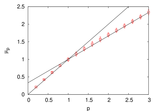
Figure 10: The exit time scaling exponents $\mu_{p}$ from Lagrangian velocity fluctuations in a DNS of thermal convection with Bolgiano-Obukhov scaling. Lines represent the bifractal prediction (71) and the error bars on the exponents have been estimated by evaluating differences in $\mu_{p}$ changing the fitting interval. Figure from BBM_POF07 .

VIII Conclusions

Starting from the seminal work of Kolmogorov we considered the statistical features (mainly scaling properties), both Eulerian and Lagrangian, of the fully developed turbulence in the framework of the multifractal model, i.e. in term of $D(h)$. The hard, still unsolved, problem is, of course, to compute $D(h)$ from first principles. Up to now the unique doable approach is to use multiplicative models motivated by phenomenological arguments. The non trivial result is the fact that, once $D(h)$ is obtained with a fit of the experimental data from the scaling exponents $\zeta_{p}$, then the other predictions obtained in the multifractal framework, e.g. the pdf of the velocity gradient, the existence of an intermediate dissipative range, the scaling of Lagrangian structure functions, are well verified.

VIII.1 Acknowledgments

We are deeply grateful to Stefano Berti, Lamberto Rondoni and Massimo Vergassola for many useful remarks. We thank Uriel Frisch and Mogens Jensen for reviewing the manuscript with useful comments. This work has been partially supported by PRIN 2005 project n. 2005027808 and by CINFAI consortium (AM).

Appendix

Appendix B Synthetic turbulence: how to generate multiaffine stochastic processes

In this Appendix we describe two methods for the generation of multi-affine stochastic signals BBCPVV93 ; BBCCV98 , whose scaling properties are fully under control. One is based on a dyadic decomposition of the signal in a wavelet basis with a suitable assigned series of stochastic coefficients BBCPVV93 . The second is based on a multiplication of sequential Langevin-processes with a hierarchy of different characteristic times BBCCV98 .
The first procedure is particularly appealing for modeling of spatial turbulent fluctuations, because of the natural identification between wavelets and eddies in the physical space. The second one looks more appropriate for mimicking the turbulent time evolution in a fixed point of the space.

Using the two methods it is possible to build a rather general $(d+1)$-dimensional process, $v({\bf x},t)$, with given scaling properties in time and in space.

B.1 An algorithm based and dyadic decomposition

A non-sequential algorithm for $1$-dimensional multi-affine signal in $[0,1]$, $v(x)$, can be introduced as BBCPVV93 :

$$v(x)=\sum_{n=1}^{N}\sum_{k=1}^{2^{(n-1)}}a_{n,k}\,\varphi\!\left(\frac{x-x_{n,k}}{\ell_{n}}\right)$$ (72)

where we have a set of reference scales $\ell_{n}=2^{-n}$ and $\varphi(x)$ is a wavelet-like function F92 , i.e. of zero mean and rapidly decaying in both real space and Fourier-space. The signal $v(x)$ is built in terms of a superposition of fluctuations, $\varphi((x-x_{n,k})/\ell_{n})$ of characteristic width $\ell_{n}$ and centered in different points of $[0,1]$, $x_{n,k}=(2k+1)/2^{n+1}$. It has been proved BBCCV98 that provided the coefficients $a_{n,k}$ are chosen by a random multiplicative process, i.e. the daughter is given in terms of the mother by a random process, $a_{n+1,k^{\prime}}=Xa_{n,k}$ with $X$ a random number identical, independent distributed for any $\{n,k\}$, then the result of the superposition is a multi-affine function with given scaling exponents, namely:

$$\langle|v(x+\ell)-v(x)|^{p}\rangle\sim\ell^{\,\zeta_{p}}\,\,,$$

with $\zeta_{p}=-p/2-\log_{2}\langle\langle X^{p}\rangle\rangle$ and $\ell_{N}\leq\ell\leq 1$. In this Appendix $\langle\langle\cdot\rangle\rangle$ indicates the average over the probability distribution of the multiplicative process.

Besides the rigorous proof, the rationale for the previous result is simply that due to the hierarchical organization of the fluctuations, one may easily see that the term dominating the expression of a velocity fluctuation at scale $R$, in (72) is given by the couple of indices $\{n,k\}$ such that $n\sim log_{2}(R)$ and $x\sim x_{n,k}$, i.e. $v(x+\ell)-v(x)\sim a_{n,k}$. The generalization (72) to d-dimension is given by:

$$v({\bf x})=\sum_{n=1}^{N}\sum_{k=1}^{2^{d(n-1)}}a_{n,k}\,\varphi\!\left(\frac{{\bf x}-{\bf x}_{n,k}}{\ell_{n}}\right)\,\,,$$

where now the coefficients $\{a_{n,k}\}$ are given in terms of a d-dimensional dyadic multiplicative process.

B.2 A sequential algorithm

Sequential algorithms look more suitable for mimicking temporal fluctuations. With the application to time-fluctuations in mind, we will denote now the stochastic 1-dimensional functions with $u(t)$. The signal $u(t)$ is obtained by a superposition of functions with different characteristic times, representing eddies of various sizes BBCCV98 :

$$u(t)=\sum_{n=1}^{N}u_{n}(t)\;.$$ (73)

The functions $u_{n}(t)$ are defined by the multiplicative process

$$u_{n}(t)=g_{n}(t)x_{1}(t)x_{2}(t)\ldots x_{n}(t)\;,$$ (74)

where the $g_{n}(t)$ are independent stationary random processes, whose correlation times are supposed to be $\tau_{n}=(\ell_{n})^{\alpha}$, where $\alpha=1-h$ (i.e. $\tau_{n}$ are the eddy-turn-over time at scale $\ell_{n}$) in the quasi-Lagrangian frame of reference LPP97 and $\alpha=1$ if one considers $u(t)$ as the time signal in a given point, and $\langle g_{n}^{2}\rangle=(\ell_{n})^{2h}$, where $h$ is the Hölder exponent. For a signal mimicking a turbulent flow, ignoring intermittency, we would have $h=1/3$. Scaling will appear for all time delays larger than the UV cutoff $\tau_{N}$ and smaller than the IR cutoff $\tau_{1}$. The $x_{j}(t)$ are independent, positive defined, identical distributed random processes whose time correlation decays with the characteristic time $\tau_{j}$. The probability distribution of $x_{j}$ determines the intermittency of the process.

The origin of (74) is fairly clear in the context of fully developed turbulence. Indeed we can identify $u_{n}$ with the velocity difference at scale $\ell_{n}$ and $x_{j}$ with $(\varepsilon_{j}/\varepsilon_{j-1})^{1/3}$, where $\varepsilon_{j}$ is the energy dissipation at scale $\ell_{j}$ BBCCV98 .

The following arguments show, that the process defined according to (73,74) is multi-affine. Because of the fast decrease of the correlation times $\tau_{j}=(\ell_{j})^{\alpha}$, the characteristic time of $u_{n}(t)$ is of the order of the shortest one, i.e., $\tau_{n}=(\ell_{n})^{\alpha}$. Therefore, the leading contribution to the structure function $\tilde{S}_{q}(\tau)=\langle|u(t+\tau)-u(t)|^{q}\rangle$ with $\tau\sim\tau_{n}$ stems from the $n$-th term in (73). This can be understood noting that in $u(t+\tau)-u(t)=\sum_{k=1}^{N}[u_{k}(t+\tau)-u_{k}(t)]$ the terms with $k\leq n$ are negligible because $u_{k}(t+\tau)\simeq u_{k}(t)$ and the terms with $k\geq n$ are sub-leading. Thus one has:

$$\tilde{S}_{q}(\tau_{n})\sim\langle|u_{n}|^{q}\rangle\sim\langle\langle|g_{n}|^{q}\rangle\rangle\langle\langle x^{q}\rangle\rangle^{n}\sim\tau_{n}^{\frac{hq}{\alpha}-\frac{\log_{2}\langle\langle x^{q}\rangle\rangle}{\alpha}}$$ (75)

and therefore for the scaling exponents:

$$\zeta_{q}={hq\over\alpha}-{\log_{2}\langle\langle x^{q}\rangle\rangle\over\alpha}\;.$$ (76)

The limit of an affine function can be obtained when all the $x_{j}$ are equal to $1$. A proper proof of these result can be found in BBCCV98 .
Let us notice at this stage that the previous “temporal” signal for $\alpha=1-h$ is a good candidate for a velocity measurements in a Lagrangian, co-moving frame of reference LPP97 . Indeed, in such a reference frame the temporal decorrelation properties at scale $\ell_{n}$ are given by the eddy-turn-over times $\tau_{n}=(\ell_{n})^{1-h}$. On the other hand, in the laboratory reference frame the sweeping dominates the time evolution in a fixed point of the space and we must use as characteristic times of the processes $x_{n}(t)$ the sweeping times $\tau_{n}^{(s)}=\ell_{n}$, i.e., $\alpha=1$.

References

References

- (1) Parisi G and Frisch U 1985 in Turbulence and predictability of geophysical fluid dynamics, Eds Ghil M Benzi R and Parisi G page 84 (Amsterdam: North-Holland)
- (2) Benzi R, Paladin G, Parisi G and Vulpiani A 1984 J. Phys. A: Math. Gen. 17 3521
- (3) Ellis R S 1999 Physica D 133 106
- (4) Varadhan S R S, in Entropy Eds Greve A Keller G and Warnecke D page 199 (Princeton: Princeton Un. Press)
- (5) Kolmogorov A N 1962 J. Fluid Mech. 13 82
- (6) Novikov E A and Stewart R W 1964 Izv. Akad. Nauk SSSR Geofiz. 3 408
- (7) Mandelbrot B B 1974 J. Fluid Mech. 62 331
- (8) Beck C and Schögl F 1995 Thermodynamics of Chaotic Systems (Cambridge: Cambridge University Press)
- (9) Badii R and Politi A 1997 Complexity: Hierarchical Structures and Scaling in Physics (Cambridge: Cambridge University Press)
- (10) Meakin P 1998 Fractals, scaling and growth far from equilibrium (Cambridge: Cambridge University Press)
- (11) Harte D 2001 Multifractals (Boca Raton: Chapman and Hall/CRC)
- (12) Halsey T C, Jensen M H, Kadanoff L P, Procaccia I and Shraiman B I, 1986 Phys. Rev. A 33 1141
- (13) Frisch U 1995 Turbulence: the legacy of A. N. Kolmogorov, (Cambridge: Cambridge University Press)
- (14) Bohr T, Jensen M H, Paladin G and Vulpiani A 1998 Dynamical systems approach to turbulence, (Cambridge: Cambridge University Press)
- (15) Monin A and Yaglom A 1971 and 1975 Statistical Fluid Dynamics, Vol. I and II (Cambridge MA: MIT Press)
- (16) Richardson L F 1922 Weather prediction by numerical processes (Cambridge: Cambridge University Press)
- (17) Kolmogorov A N 1941 Dokl. Akad. Nauk. SSSR 30 299; reprinted in Kolmogorov A N 1991 Proc. R. Soc. Lond. A 434 9.
- (18) Anselmet F, Gagne Y, Hopfinger E J and Antonia R A 1984 J. Fluid. Mech. 140 63
- (19) Paladin G and Vulpiani A 1987 Phys. Rep. 156 147
- (20) She Z S and Lévêque E 1994 Phys. Rev. Lett. 72 336
- (21) Aurell E Frisch U Lutsho J and Vergassola M 1992 J. Fluid Mech. 238 467
- (22) Bender C M and Orszag S A 1999 Advanced mathematical methods for scientists and engineers, (New York: Springer)
- (23) Frisch U, Martins Afonso M, Mazzino A and Yakhot V 2005 J. Fluid Mech. 542 97
- (24) Meneveau C and Sreenivasan K R 1989 Phys. Lett. A 137 103
- (25) van de Water W and Schram P 1988 Phys. Rev. A 37 3118
- (26) Paladin G and Vulpiani A 1987 Phys. Rev. A. 35 1971
- (27) Frisch U and Vergassola M 1991 Europhys. Lett. 14 439
- (28) Frisch U and She Z -S 1991 Fluid Dynamic Research 8 139
- (29) Castaing B, Gagne Y and Hopfinger E J 1990 Physica D 46 177
- (30) Vincent A and Meneguzzi M 1991 J. Fluid Mech. 225 1
- (31) Benzi R, Biferale L, Paladin G, Vulpiani A and Vergassola M 1991 Phys. Rev. Lett 67 2299
- (32) Gagne Y and Castaing B 1991 C. R. Acad. Sci Serie II 312 441
- (33) Biferale L, Cencini M, Vergni D and Vulpiani A 1999 Phys. Rev. E 60 R6295
- (34) Jensen M H 1999 Phys. Rev. Lett. 83 76
- (35) Boffetta G, Cencini M, Falcioni M and Vulpiani A 2002 Phys. Reports 356, 367.
- (36) Jensen M H, Paladin G and Vulpiani A 1991 Phys. Rev. Lett. 67 208
- (37) Shraiman B I and Siggia E D 2000 Nature 405 639
- (38) Lamb H 1945 Hydrodynamics (New York: New York Dover Publ.)
- (39) Tritton D J 1988 Physical fluid dynamics, (Oxford: Oxford Science Publ.)
- (40) Maxey M R and Riley J J 1983 Phys. Fluids 26 883
- (41) Bec J, Biferale L, Cencini M, Lanotte A S and Toschi F 2006 Phys. Fluids 18 081702
- (42) Hénon M 1966 C. R. Acad. Sci. Paris A 262 312
- (43) Aref H 1984 J. Fluid Mech. 143 1
- (44) Chandrasekhar S 1943 Rev. Mod. Phys. 15 1
- (45) Tennekes H and Lumley J L 1972 A First Course in Turbulence (Cambridge MA: MIT Press)
- (46) Borgas M S 1993 Phil. Trans. R. Soc. Lond. A 342 379
- (47) Boffetta G, De Lillo F and Musacchio S 2002 Phys. Rev. E 66 066307
- (48) Mordant N, Metz P, Michel O and Pinton J F 2001 Phys. Rev. Lett. 87 214501
- (49) Biferale L, Boffetta G, Celani A, Lanotte A and Toschi F 2006 J. Turbulence 7 N6
- (50) Biferale L, Boffetta G, Celani A, Lanotte A and Toschi F 2005 Phys. Fluids 17 021701
- (51) Benzi R, Ciliberto S, Tripiccione R, Baudet C, Massaioli F and Succi S 1993 Phys. Rev. E 48 R29
- (52) La Porta A, Voth G A, Crawford A M, Alexander J and Bodenschatz E 2001 Nature 409 1017
- (53) Biferale L, Boffetta G, Celani A, Devenish B J Lanotte A and Toschi F 2004 Phys. Rev. Lett. 93 064502
- (54) Richardson L F 1926 Proc. R. Soc. London A 110 709
- (55) Batchelor G K 1952 Proc. Camb. Phil. Soc. 48 345
- (56) Obukhov A 1941 Izv. Akad. SSSR. Ser. Geogr. Geofiz. 5 453
- (57) Boffetta G and Sokolov I M 2002 Phys. Fluids 14 3224
- (58) Boffetta G, Celani A, Crisanti A and Vulpiani A 1999 Phys. Rev. E 60 6734
- (59) Artale V, Boffetta G, Celani A, Cencini M and Vulpiani A 1997 Phys. Fluids A 9 3162
- (60) Boffetta G and Sokolov I M 2002 Phys. Rev. Lett. 88 094501
- (61) Biferale L, Boffetta G, Celani A, Devenish B J, Lanotte A and Toschi F 2005 Phys. Fluids 17 115101
- (62) Bistagnino A, Boffetta G and Mazzino A 2007 Phys. Fluids 19 011703
- (63) Ott S and Mann J 2000 J. Fluid Mech. 422 207
- (64) Siggia E D 1994 Annu. Rev. Fluid Mech. 26 137
- (65) Chertkov M 2003 Phys. Rev. Lett. 91, 115001
- (66) Zhang J, Wu X L and Xia K Q 2005 Phys. Rev. Lett. 94 174503
- (67) Celani A, Mazzino A and Vergassola M 2001 Phys. Fluids 13 2133
- (68) Biferale L, Cencini M, Lanotte A, Vergni D and Vulpiani A 2001 Phys. Rev. Lett. 87 124501
- (69) Benzi R, Biferale L, Crisanti A, Paladin G, Vergassola M and Vulpiani A 1993 Physica D 65 352
- (70) Biferale L, Boffetta G, Celani A, Crisanti A and Vulpiani A 1998 Phys. Rev. E 57 R6261
- (71) Farge M 1992 Ann. Rev. Fluid Mech. 24 395
- (72) L’vov V S, Podivilov E and Procaccia I 1997 Phys. Rev. E 55 7030