Quantum transport in ferromagnetic Permalloy nanostructures

Abstract

We studied phase coherent phenomena in mesoscopic Permalloy samples by exploring low temperature transport. Both, differential conductance as a function of bias voltage and magnetoconductance of individual wires display conductance fluctuations. Analysis of these fluctuations yields a phase coherence length of $\sim 250$ nm at 25 mK as well as a $1/\sqrt{T}$ temperature dependence. To suppress conductance fluctuations by ensemble averaging we investigated low temperature transport in wire arrays and extended Permalloy films. In these samples we have measured conductance corrections which stem from electron-electron interaction (EEI) but attempts to detect signatures of weak localization were without success.

I Introduction

In nanoscale samples the conductance is affected by quantum interference effects at sufficiently low temperatures, including weak localization (WL) Bergmann , universal conductance fluctuations (UCF) Lee or Aharonov-Bohm oscillations Aharonov . All these effects rely on the electron’s wave nature and require phase coherent transport over a certain distance. In nonmagnetic metals interference effects have been investigated intensely over the last two decades (for a review see, e.g., reference Imry ), showing that the electrons can propagate up to several microns without losing their phaseinformation, although their mean free path is much smaller. For ferromagnetic metals, in contrast, only a few experimental works on phase coherent phenomena exist (e.g. Wei ; Kasai ; Lee3 ). While Aharonov-Bohm oscillations or universal conductance fluctuations have been observed in Permalloy Kasai and cobalt devices Wei , the suppression of weak localization is still an open question. Up to now no clear signature of weak localization was found in any ferromagnetic metal. For example, the conductance of Co Brands ; Wei , Co/Pt multilayers Brands3 , Fe Brands2 and Ni Ono was not affected by weak localization. In these materials a decreasing conductance with decreasing temperature was ascribed to electron-electron interaction Brands ; Wei ; Brands3 ; Brands2 ; Ono . However, in the ferromagnetic semiconductor (Ga,Mn)As Ohno weak localization corrections could be observed quite recently WL ; Rozkinson . In conmtrast to ferromagnetic metals the internal magnetic induction of (Ga,Mn)As is rather small. In this work we will investigate universal conductance fluctuations, weak localization and electron-electron interaction in Permalloy nanostructures.

II Sample preparation and measurement technique

For the experiments we fabricated single wires, arrays of wires connected in parallel and thin film areas using electron beam lithography (a Zeiss electron microscope equipped with a nanonic pattern generator) and thermal evaporation of Permalloy. The contacts to the samples were made out of gold after a brief in-situ ion beam etching to remove the oxide. An electron micrograph of a 145 nm long, 35 nm wide and 15 nm thick Permalloy wire is shown in figure 1a.

All measurements have been performed in a top-loading dilution refrigerator using standard 4 probe lock-in techniques. The external magnetic field was always applied perpendicular to the plane. To avoid heating of the electrons careful shielding as well as small measuring currents (dependending on the sample’s resistance ranging from 4 nA to 400 nA) were crucial. To measure the differential resistance we also used standard lock-in techniques. A DC-voltage $U_{DC}$ was superimposed upon a comparably small AC-voltage $U_{AC}$ ($5$ $\mu$V) having a frequency of 417 Hz. The conductance $G$ was obtained by inverting the resistance $R$ of the samples $G=1/R$, while the differential conductance was obtain by inverting the differential resistance $G^{d}=1/R^{d}=1/($d$U/$d$I)$.

III Universal conductance fluctuations in single wires

Universal conductance fluctuations (UCF) result from correlations between different transmission paths through a disordered mesoscopic sample (Washburn and references therein). Hence the conductance $G$ of a mesoscopic sample is sensitive to the impurity configuration. Changing the applied magnetic field $B$ or the applied bias voltage $U$ leads to aperiodic conductance fluctuations Washburn . While changing in the magnetic field leads to a relative phase shift of different paths due to the Aharonov-Bohm-effect, a change in bias voltage changes the electron’s energy and thus the corresponding wavelength. For observing UCF, phase coherence is necessary. If the sample is larger than the phase coherence length in one or more spatial dimensions the fluctuations get damped until the classical value of conductance is reached Lee . Hence sufficiently small samples and low temperatures are required to observe universal conductance fluctuations.

Here we investigate conductance fluctuations in differential conductance $G^{d}(U)$ and in magnetoconductance $G(B)$ of two single Py wires having a length of 145 nm and 330 nm respectively. The width of both wires is 35 nm and the thickness is 15 nm. An electron micrograph of the 145 nm long wire is shown in figure 1a.

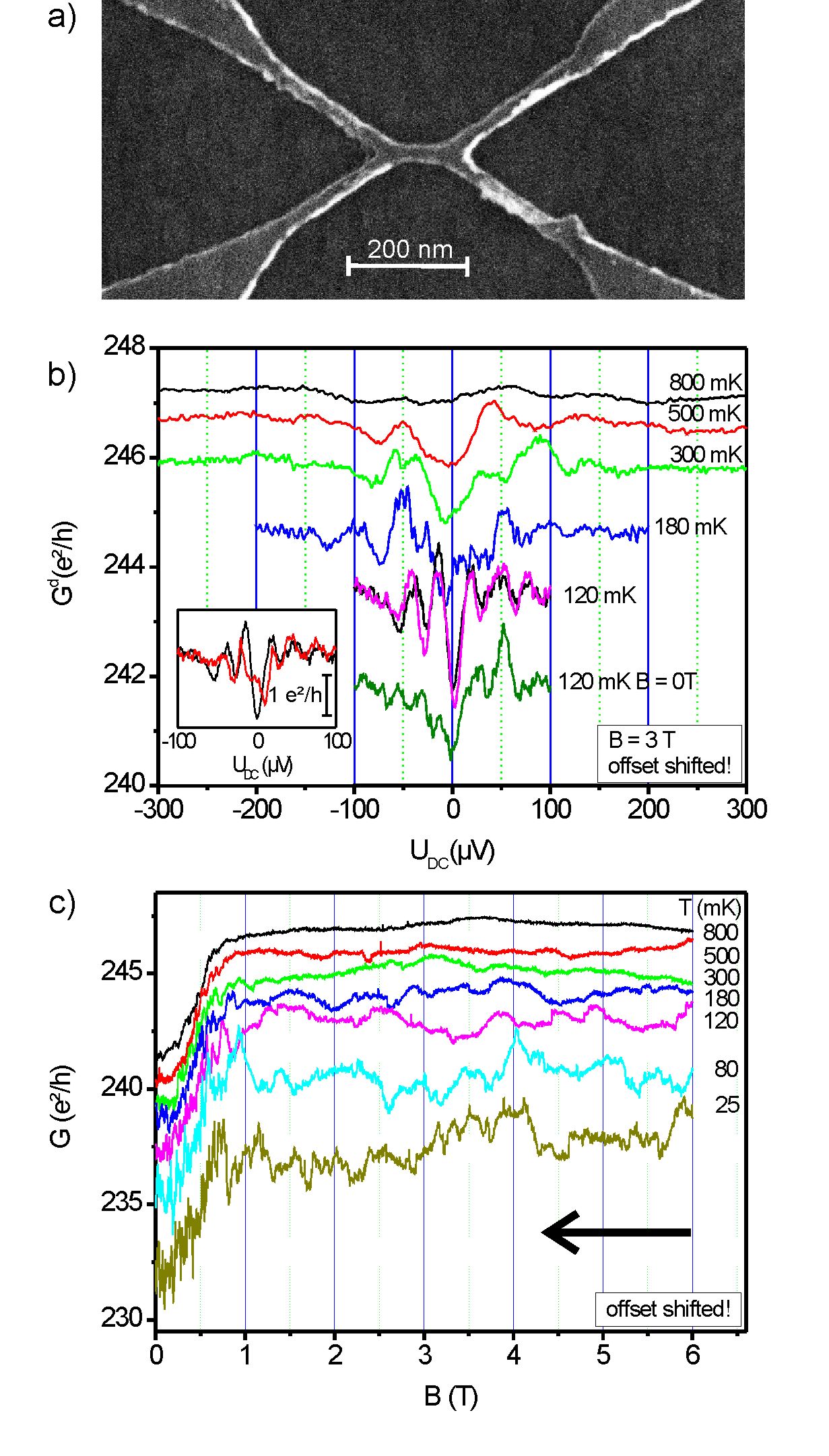
Figure 1: a) Electron micrograph of the 145 nm long Permalloy wire. b) Differential conductance of the 145 nm long Permalloy wire measured at different temperatures. The applied magnetic field was 3 T (except for the lowest trace: Here $B=0$.). The different traces, except the 800 mK trace, were shifted for clarity. The reproducibility is shown for the 120 mK trace (purple and black trace). The inset shows the differential conductance at 120 mK and 3 T before and after the field was raised to 4 T. The black trace in the inset corresponds to the black trace at 120 mK in the main figure. c) Magnetoconductance of the 145 nm long wire in a perpendicular applied magnetic field at different temperatures. Also here, the different traces, except the 800 mK trace, were shifted for clarity. The arrow gives the sweeping direction.

The differential conductance $G^{d}(U_{DC})$ as a function of the applied bias voltage $U_{DC}$ of the 145 nm long wire is shown in figure 1b for temperatures $T$ ranging from 120 mK to 800 mK. The magnetic field applied normal to the sample was 3 T (except for the lowest trace: Here $B=0$). At all temperatures fluctuations in the differential conductance are visible, showing that phase coherent transport takes place in the wire. The reproducibility of the differential conductance is demonstrated for the $T=120$ mK trace. With increasing temperature the fluctuation amplitude gets reduced. This shows that the sample is larger than the phase coherence length at least at 180 mK. Also with increasing DC-voltage the amplitude of the fluctuations decreases. This suggests that the applied voltage causes heating. The correlation voltage $U_{C}$, the average spacing between maxima and minima, gives the energy, which is necessary to change the electron’s phase by $\pi$. Here $U_{C}$ increases with increasing temperature. The correlation voltage is related to the dephasing time $\tau_{\phi}$ by: $|e|U_{C}=\hbar/\tau_{\phi}$ Datta . Hence the dephasing time decreases with increasing temperature as expected Lin . At $T=120$ mK the correlation voltage is approx. 17 $\mu$V. This corresponds to a dephasing time of 40 ps. With the diffusion constant of Permalloy $D\approx 4\cdot 10^{-4}$ m²/Vs Kasai2 we obtain for the phase coherence length $L_{\phi}=\sqrt{D\tau_{\phi}}=130$ nm at 120 mK. For comparison: The thermal energy $k_{B}T=10$ $\mu$eV at 120 mK. Hence thermal broadening does not lead to a suppression of interference as $k_{B}T<eU_{C}$ Beenakker .

To investigate the temperature dependency of the dephasing time we plotted the correlation voltage of the 145 nm long wire in a log-log diagram versus temperature (see inset of figure 2). The slope of the correlation voltage can be approximated by 1. This corresponds to a dephasing time $\tau_{\phi}\propto 1/T$ and thus to a phase coherence length $L_{\phi}\propto 1/\sqrt{T}$. We note that the estimate of the correlation voltage is associated with a relatively high degree of uncertainty, as only the region around zero voltage can be used for an estimate of $U_{C}$. Hence the slope gives only a rough estimate of the temperature dependency.

The differential conductance of the 330 nm long wire also exhibits reproducible fluctuations associated with phase coherent transport (not shown). At $T=120$ mK the correlation voltage in the 330 nm long wire is 20 $\mu$V, which is quite close to the correlation voltage observed in the 145 nm long wire at the same temperature. Hence the dephasing time and the phase coherence length are quite similar in both wires, as the measurement of the correlation voltage gives the dephasing time independent of the sample’s geometry. In the 330 nm long wire the temperature dependence of the correlation voltage couldn’t be estimated properly as the fluctuations disappear above 180 mK. This is due to damping of the conductance fluctuations with increasing sample size. The correlation voltage taken at $T=120$ mK and $T=180$ mK give a temperature dependency in good agreement with the one obtained in the 145 nm long wire (see inset of figure 2).

In mesoscopic samples reproducible conductance fluctuations are also visible in the magnetoconductance $G(B)$, also known as magnetic fingerprint of the sample Lee . In figure 1c the magnetoconductance of the 145 nm long wire is shown for temperatures ranging from 25 mK to 800 mK, exhibiting conductance fluctuations vanishing with increasing temperature. The positive magnetoconductance at $B=0...0.7$ T is due to the anisotropic magnetoresistance (AMR) in ferromagnets McGuire . For a magnetization aligned in wire direction (here the easy magnetic axis) the conductance is smaller than for perpendicular orientation (here a hard magnetic axis). In contrast to fluctuations of the differential conductance, the magnetoconductance fluctuations are not reproducible within several sweeps. As the conductance fluctuations only appear at low temperatures and decrease with increasing temperature and increasing wire length, we ascribe them to phase coherent phenomena. To check whether the fluctuations originate from time dependent fluctuations, we measured the conductance at a fixed magnetic field for the time interval of a magnetic field sweep. Time dependent fluctuations are visible, but their amplitude is by approx. a factor of 4 lower compared to the magnetoconductance fluctuations. Additionally, the time scale of fluctuations is longer in the time-sweep compared to the magnetic field sweep. Hence we can conclude that the observed conductance fluctuations, shown in figure 1c, are primarily due to changes of $B$ but only superimposed by time depending fluctuations. Time dependent universal conductance fluctuations in Permalloy nanowires are in the focus of reference Lee3 . A possible explanation for irreproducible magnetoconductance traces could be a change of the scatterer configuration due to magnetostriction. While the fluctuations in the differential conductance are well reproducible for a fixed magnetic field (see figure 1b), they get less reproducible when the magnetic field is changed between the measurements. This is shown in figure 1b. The two traces in the inset show the differential conductance at $T=120$ mK and $B=3$ T. Between the measurements the magnetic field was increased to 4 T and then reduced to 3 T again (the black trace shows the differential conductance at the beginning and the red trace after the magnetic field was varied). This magnetic field change reduces the reproducibility of the traces compared to the two traces shown in figure 1b at 120 mK (black and purple), where the magnetic field was not changed between the measurements. Hence, a change in the impurity configuration due to magnetostriction is a possible candidate for the origin of the observed irreproducibility.

Figure 2: Amplitude of conductance fluctuations $dG_{rms}$ measured in the magnetoconductance of the 145 nm long (black squares) and 330 nm long wire (red circles). The lines are a guide for the eyes and give a slope of $a=-0.84$. The inset shows the correlation voltage of both wires for different temperatures. Also here black squares correspond to the 145 nm long wire and red circles to the 330 nm long wire. The straight line is a guide for the eyes and gives a slope of $a=1$.

In the low field region ($|B|<0.7$ T), the region where the magnetization rotates from in plane to perpendicular to the plane, the conductance fluctuations are more pronounced than in the high field region. Such a behavior has already been observed in (Ga,Mn)As wires Konni ; Vila and ad hoc ascribed to the formation of domain walls Vila . Analyzing the fluctuations in the differential conductance at zero magnetic field (figure 1b, lowest trace) one finds, that neither the amplitude nor the correlation voltage is significantly different compared to $B=3$ T. This implies that the dephasing time is not much affected due to the presence of domain walls in the low field region. A similar result was found in reference Lee3 analyzing time dependent universal conductance fluctuations (TDUCF) in Permalloy nanowires. Their analysis of TDUCFs supports the idea that domain walls act as coherent scatterers Lee3 . In the following the analysis is limited to high magnetic fields ($B=1...6$ T), where the magnetization is saturated perpendicular to the plane.

The root mean square amplitude of the conductance fluctuations $dG_{rms}$ of the 145 nm and 330 nm long wires (taken at $B=1...6$ T) is plotted in a log-log diagram versus $T$ in figure 2. Here $dG_{rms}=\sqrt{\langle(G-\langle G\rangle)^{2}\rangle}$, where $\langle...\rangle$ denotes averaging over $B$. For a quasi one dimensional wire ($w,t<L_{\phi}<l$) one finds for the amplitude of the conductance fluctuations Lee :

$$dG_{rms}=C\frac{e^{2}}{h}\left(\frac{L_{\phi}}{l}\right)^{3/2}.$$ (1)

Here, $l$ is the wire length and $C$ is a constant, with a value close to or smaller than unity, depending, e.g., on the strength of spin-orbit coupling Chandrasekhar and the applied magnetic field Lee . Equation (1) is applicable to describe the conductance fluctuations as long as thermal averaging can be ruled out: $L_{\phi}<L_{T}=\sqrt{\hbar D/k_{B}T}$, which is equivalent to $eU_{C}>k_{B}T$. In our Permalloy wire this is the case as shown above and equation (1) can be used to extract the phase coherence length. $dG_{rms}$ of the 145 nm long wire is increasing with decreasing temperature until it starts to saturate at 80 mK at a value of 0.5 $e^{2}/h$ (see figure 2). For such a saturation, there are essentially three possible reasons:

1. The effective electron temperature is higher than the bath temperature due to a too high measuring current or external RF-noise.

2. Magnetic impurities lead to a saturation of $L_{\phi}$ due to Kondo-scattering as observed in normal metals Pierre .

3. The phase coherence length reaches the wire length and the wire is no longer quasi one dimensional. In that case $dG_{rms}=Ce^{2}/h$ Lee .

As we deal here with a ferromagnet and since saturation is only observed in the shorter one of the two wires, an intrinsic saturation of the phase coherence length due to Kondo-scattering, is unlikely. While the amplitude of the conductance fluctuations of the 25 mK and the 80 mK trace in figure 1c is the same, the correlation field $B_{C}$ is smaller at 25 mK. The correlation field defines the typical field scale on which the conductance fluctuates and is related to the maximum area enclosed by a phase coherent trajectory. In one dimensional samples $B_{C}=\frac{h}{e}\frac{1}{wL_{\phi}}$ Lee . We note that the correlation field might not be a well defined quantity here, as the impurity configuration might be changed by magnetostriction, as discussed above. Hence the correlation field can only serve as a very rough estimate of the phase coherence length. At 80 mK the correlation field is between $\sim$0.6 T and $\sim$0.8 T. This corresponds to a phase coherence length of $\sim$150-200 nm. When extrapolating the correlation voltage $U_{C}$ (see inset of figure 2) down to 80 mK, one arrives at a phase coherence length of 160 nm. This is in very good agreement with the phase coherence length estimated from the correlation field. Hence, the saturation of $dG_{rms}$ observed in the 145 nm long wire below 80 mK is most likely due to an dimensional cross-over from quasi 1-D to 0-D and the saturation value of $dG_{rms}$ is $\sim 0.5e^{2}/h$.

In both wires the temperature dependency of $dG_{rms}$ can be approximated by a power law: $dG_{rms}\propto T^{-0.84}$. Using equation (1), the temperature dependency of the dephasing length is: $L_{\phi}\propto T^{-0.55}$. This temperature dependency agrees well with the one estimated using the correlation voltage $U_{C}$ ($L_{\phi}\propto T^{-0.5}$). In Permalloy wires noise measurements reveal a temperature dependency of $L_{\phi}$ probably steeper than $T^{-0.5}$ Lee3 , but the analysis was complicated by several uncertainties. Also the wires investigated in Lee3 were quasi two dimensional, because of the higher temperature ($T>2$ K). Hence a direct comparison is difficult. In ferromagnetic (Ga,Mn)As wires the phase coherence length followed a $T^{-0.5}$ dependency Konni ; Vila and was associated with critical electron-electron-scattering (CEEI) Konni ; Review ; Dai . For Permalloy CEEI seems not to be a suitable candidate for dephasing as CEEI describes dephasing in a strongly disordered metal near the metal insulator transition (MIT). In metals far away from the MIT dephasing is usually ascribed to Nyquist scattering leading to a phase coherence length $\propto T^{-1/3}$ in 1-D systems Altshuler . So, the microscopic mechanism of dephasing in Permalloy remains an open issue.

The value of the phase coherence length at 25 mK is approx. 250 nm. We arrive at this value by analyzing the magnetoconductance fluctuations of the 330 nm long wire ($L_{\phi}=180$ nm) or by extrapolating the magnetoconductance fluctuations of the 145 nm long wire down to 25 mK ($L_{\phi}=260$ nm). We note that there is some uncertainty in determining the length of the wires, especially in the region of the voltage probes, where the wire widens up. This uncertainty enters the phase coherence length linearly. Taking the correlation energy and extrapolating the value of $U_{C}$ down to 25 mK leads to a phase coherence length of $\sim$260 nm (145 nm long wire) and $\sim$240 nm (330 nm long wire). This approximation is independent on the exact wire geometry. In reference Kasai the phase coherence length in Permalloy was extracted from periodic Aharonov-Bohm oscillations. Their value of $L_{\phi}=500$ nm taken at 30 mK, is by a factor of 2 larger than the value estimated here. The difference might be explained by the different material used. The saturation field of the magnetization observed in a perpendicular external field, defined by the saturation field of the AMR is in reference Kasai $\sim 1.2$ T. For Permalloy (Ni₈₁Fe₁₉) the saturation magnetization is 1.0 T. Hence the saturation field is 1.0 T in an extended film and 0.5 T in a cigar shaped ellipsoid with infinite aspect ratio (comparable to a long wire with a very small cross-section) and with the long axis perpendicular to the external field Hubert . For the geometry used in reference Kasai (a 2.5 $\mu$m long wire with a cross-section of $40\times 20$ nm², having a ring of 500 nm diameter and the same cross-section in the middle; see reference Kasai for details) one would expect a saturation field above, but still close to 0.5 T. In our samples the saturation field is $\sim 0.7$ T in the 145 nm and 330 nm long wires (see figure 1c), $\sim 1.0$ T in the extended film (see inset of figure 3a) and $\sim 0.6$ T in the wire array (see inset of figure 3b). These values are consistent with the ones expected for Permalloy. Hence the material used in reference Kasai seems to be quite different from the material used here and the values of the phase coherence length can hardly be compared.

IV Electron-electron interaction in 1D and 2D samples

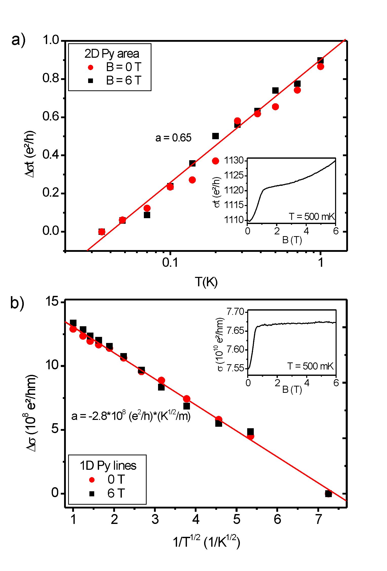
Figure 3: a) Change in conductivity $\Delta\sigma$ multiplied with the layer thickness $t$ of the two-dimensional square at zero field (red circles) and $B=6$ T (black squares) plotted versus log$T$. The line is the best linear fit of the 6 T data and has a slope of 0.65. The inset shows the magnetoconductance at $T=500$ mK. b) Conductivity change of a quasi one dimensional line array at zero field (red circles) and $B=6$ T (black squares) plotted versus $1/\sqrt{T}$. The line is the best linear fit of the 6 T data and has a slope of $-2.8\cdot 10^{8}$ (e²/h)$\cdot(\sqrt{\mathrm{K}}/$m). The inset shows the magnetoconductance at $T=500$ mK.

At low temperatures quantum interference effects like weak localization (WL) Bergmann or electron-electron interaction (EEI) Lee2 lead to a reduction of the conductance even in macroscopic samples. The effect of weak localization originates from the constructive interference of partial waves traveling on time reversed paths. This leads to an increased probability of backscattering and hence reduces the conductance. As a magnetic field removes time-reversal symmetry, weak localization gets suppressed in the presence of a magnetic field and the corresponding magnetoconductance is positive Bergmann . In Permalloy wires and films a positive magnetoconductance in a perpendicular magnetic field, as expected for WL, is already present due to the anisotropic magnetoresistance (AMR) McGuire . But in contrast to WL the AMR is independent of the temperature, at least below 1 K, and thus does not lead to a change in conductivity with decreasing temperature. Electron-electron interaction, on the other hand, arises from a modified screening of the Coulomb potential due to the diffusive propagation Lee2 . The size and the temperature dependency of the conductivity correction are very similar for EEI and WL at zero field Lee2 , but in contrast to WL, EEI is not suppressed by a magnetic field. Hence the different effects (AMR, WL and EEI) can be distinguished quite effectively by comparing the conductivity decrease at different magnetic fields. In case of WL the conductivity at zero field is expected to decrease more precipitously with decreasing $T$ compared to the case with finite $B$.

As ferromagnets have an internal magnetic induction, the question arises whether WL can be observed in a ferromagnet at all. Up to now several experimental works explore this question, showing that WL is absent in Co Brands ; Brands2 , Fe Brands2 , Ni Ono and Co/Pt multilayers Brands3 . In the ferromagnetic semiconductor (Ga,Mn)As, having a rather small internal magnetic induction, weak localization was observed WL ; Rozkinson . As theory claims that WL gets not suppressed by internal magnetic induction Dugaev ; Sil , the question arises why WL can be observed in (Ga,Mn)As but not in Co, Fe, Ni, or Co/Pt multilayers. One important difference between these materials is the phase coherence length. While $L_{\phi}\approx 160$ nm at 20 mK is quite large in (Ga,Mn)As Review , the phase coherence length is comparably small in Co ($L_{\phi}\approx 30$ nm at 30 mK Wei ) and Ni ($L_{\phi}\approx 80$ nm at 30 mK Kasai2 ). Hence Permalloy is a quite promising candidate for exploring WL as it combines a strong internal magnetic induction ($H_{Int}=1.0$ T compared to 40 mT in (Ga,Mn)As Ohno ) with a relatively large phase coherence length of approx. 250 nm at 25 mK.

To study Permalloy for WL/EEI experiments, we fabricated an extended square ($w=l=4$ $\mu$m, $t=$15 nm) and an array of 6 wires in parallel ($w=20$ nm, $l=4$ $\mu$m, $t=15$ nm) and measured their conductivity at different temperatures with and without an applied perpendicular magnetic field. The square is expected to behave quasi two-dimensional, as $w,l>L_{\phi},L_{T}>t$ and the wire array is expected to behave quasi one-dimensional, as $l>L_{\phi},L_{T}>w,t$ at temperature below 1 K. The magnetoconductance of the square and the wire array are shown in the insets of figure 3 for $T=500$ mK. Due to ensemble averaging universal conductance fluctuations are suppressed in both systems. For both samples the AMR is visible up to 1 T (area) and 0.6 T (wires) as expected for Permalloy and the corresponding saturation fields Hubert . The temperature dependency of the conductivity change of the area, relative to $T=35$ mK, is shown in figure 3a for $B=6$ T (black squares) and zero field (red circles). At both magnetic fields the conductivity follows a logarithmical temperature dependency with a slope independent of the applied magnetic field. Hence WL can be ruled out as origin of the conductivity decrease, as WL gets suppressed by an external field. EEI interaction leads to a conductivity decrease independent of the applied magnetic field. For the conductivity decrease due to EEI one obtains in two-dimensional films Lee2 :

$$\Delta\sigma t=\frac{F^{2D}}{\pi}\frac{e^{2}}{h}\mathrm{log}\frac{T}{T_{0}},$$ (2)

with a screening factor $F^{2D}$. In our Permalloy square one obtains a screening factor $F^{2D}=2.0$, using a slope of 0.65 as shown in figure 3a. This value of $F^{2D}$ is in excellent agreement with the screening factors found in other ferromagnets: For Co $F^{2D}=2.0...2.6$ Brands ; Brands2 , for (Ga,Mn)As $F^{2D}=1.8...2.6$ EEI and for Co/Pt multilayers $F^{2D}=2.5$ Brands3 . In Fe and Ni the screening factors are comparable to the screening factor observed in Co Brands2 . We note that the effect of EEI is rather small in the quasi two-dimensional film. The relative conductivity change $\Delta\sigma/\sigma$ from 1 K to 35 mK is only $\sim 8\cdot 10^{-4}$.

The magnetoconductance of the wire array, taken at 500 mK, is shown in the inset of figure 3b. Also in the wire array the AMR is visible but saturates already at $\approx 0.6$ T. This is due to the different shape anisotropy compared to an extended film Hubert . The conductivity decrease with respect to 20 mK is plotted in figure 3b for $B=6$ T and zero field. Also in the wire array the conductivity decrease is independent of the applied magnetic field. Hence WL is absent also in the wire array. The temperature dependency of the conductivity decrease is rather different in the wire array and the Py-square. In the wire array $\Delta\sigma$ follows a $1/\sqrt{T}$ dependency as it is expected for EEI in quasi one-dimensional samples Lee2 :

$$\Delta\sigma=-\frac{F^{1D}}{\pi A}\frac{e^{2}}{\hbar}\sqrt{\frac{\hbar D}{k_{B}T}},$$ (3)

with a screening factor $F^{1D}$, the wire cross-section A and the thermal diffusion length $L_{T}=\sqrt{\frac{\hbar D}{k_{B}T}}$. Using $D=4\cdot 10^{-4}$ m²/Vs Kasai2 and $\delta\sigma\sqrt{T}=-2.8\cdot 10^{8}$ (e²/h)$\cdot$($\sqrt{\mathrm{K}}$/m) (see figure 3b) one obtains as screening factor: $F^{1D}=0.77$. Also the screening factor $F^{1D}$ is in excellent agreement compared to the screening factors obtained for other quasi 1-D ferromagnets ($F^{1D}=0.83$ in Ni Ono and $F^{1D}=0.72...0.80$ in (Ga,Mn)As EEI ). In the quasi one-dimensional wire array the effect of EEI becomes quite large compared to the quasi two-dimensional film, as predicted by theory Lee2 . In 1D the conductivity decreases by approx. 1.1 % from 1 K to 35 mK. This is by a factor of 14 larger than the conductivity decrease in the quasi two-dimensional film.

V Summary

We investigated quantum interference effects in mesoscopic Permalloy films and wires at milikelvin temperatures. Our analysis of universal conductance fluctuations in single wires reveals a phase coherence length of $\sim 250$ nm at 25 mK. Compared to other ferromagnets this value is relatively large (In Co $L_{\phi}=30$ nm at 30 mK Wei , in Ni $L_{\phi}=80$ nm at 30 mK Kasai2 ). A possible explanation was given by Kasai et al. Kasai2 : In ferromagnets the phase coherence length gets probably reduced with increasing magnetocrystalline anisotropy energy. The observed temperature dependency of the dephasing time $\propto T^{-1/2}$ is stronger than expected for Nyquist scattering in 1-D systems Altshuler ($\propto T^{-1/3}$). A similar result was already obtained by Lee et al. Lee3 investigating TDUCF in Permalloy. A microscopic mechanism for the $T^{-1/2}$ temperature dependence is still missing. Although the phase coherence length is relatively large, the conductance in 1-D and 2-D Permalloy is not affected by weak localization. The decreasing conductance with decreasing temperature can be well described by EEI, as already shown for other ferromagnetic metals Brands ; Brands2 ; Brands3 ; Ono . The excellent agreement of the screening factors found in the ferromagnets investigated up to now, underline the universal character of EEI. The size of the WL correction is expected to be of the same order as EEI at zero field Lee2 . Hence our data show that WL is strongly suppressed or even absence in Permalloy. The absence of a Cooperon contribution in Permalloy, the process leading to WL, has already been proposed by Lee et al. investigating TDUCF Lee3 . Although theory predicts the existence of WL in ferromagnets Dugaev ; Sil , it seems that the Cooperon contribution is suppressed in ferromagnets, independent on the value of the phase coherence length. The process which could lead to such a suppression is still unknown. Hence, further investigations, experimental as well as theoretical, are necessary to clarify the role of the internal magnetic induction on the phase coherent transport in general, and on the Cooperon in particular.

Acknowledgement: This work was financially supported by the Deutsche Forschungsgemeinschaft (DFG) via SFB 689.

References

- (1) G. Bergmann, Phys. Rep. 107, 1 (1984).
- (2) P. A. Lee, A. D. Stone, and H. Fukuyama, Phys. Rev. B 35, 1039 (1987).
- (3) Y. Aharonov and D. Bohm, Phys. Rev. 115, 485 (1959).
- (4) Y. Imry, Introduction to mesoscopic Physics (Oxford University Press, Oxford, 1997).
- (5) Y.G. Wei, X. Y. Liu, L. Y. Zhang, and D. Davidović, Phys. Rev. Lett. 96, 146803 (2006).
- (6) S. Kasai, E. Saitoh, and H. Miyajima, Appl. Phys. Lett. 81, 316 (2002).
- (7) S. Lee, A. Trionfi, and D. Natelson, Phys. Rev. B 70, 212407 (2004).
- (8) M. Brands, C. Hassel, A. Carl, and G. Dumpich, Phys. Rev. B 74, 033406 (2006).
- (9) M. Brands, A. Carl, and G. Dumpich, Annalen der Physik 14, 745 (2005).
- (10) M. Brands, A. Carl, O. Posth, and G. Dumpich, Phys. Rev. B 72, 085457 (2005).
- (11) T. Ono, Y. Ooka, S. Kasai, H. Miyajima, K. Mibu and T. Shinjo, J. Magn. Magn. Mater. 226, 1831 (2001).
- (12) P. A. Lee and T. V. Ramakrishnan , Rev. Mod. Phys. 57, 287 (1985).
- (13) H. Ohno, A. Shen, F. Matsukura, A. Oiwa, A. Endo, S. Katsumoto, and Y. Iye, Appl. Phys. Lett. 69, 363 (1996).
- (14) D. Neumaier, K. Wagner, S. Geißler, U. Wurstbauer, J. Sadowski, W. Wegscheider, and D. Weiss, Phys. Rev. Lett. 99, 116803 (2007).
- (15) L. P. Rokhinson, Y. Lyanda-Geller, Z. Ge, S. Shen, X. Liu, M. Dobrowolska, and J. K. Furdyna, Phys. Rev. B 76, 161201(R) (2007).
- (16) S. Washburn and R. A. Webb, Rep. Prog. Phys. 55, 1311 (1992).
- (17) S. Datta, Electronic Transport in Mesoscopic Systems, edited by A.L. Efros and M. Pollak (Elsevier, New York, 2002).
- (18) J. J. Lin and J. P. Bird, J. Phys.: Condens. Matter 14, R501 (2002).
- (19) S. Kasai, S. Saitoh, and H. Miyajima, J. Appl. Phys. 93, 8427 (2003).
- (20) C. W. J. Beenakker and H. van Houten, Solid State Phys. 44, 1 (1991).
- (21) T. R. McGuire and R. I. Potter, IEEE Trans. Magn. MAC-11, 1018 (1975).
- (22) K. Wagner, D. Neumaier, M. Reinwald, W. Wegscheider, and D. Weiss, Phys. Rev. Lett. 97, 056803 (2006).
- (23) L. Vila, R. Giraud, L. Thevenard, A. Lemaître, F. Pierre, J. Dufouleur, D. Mailly, B. Barbara, and G. Faini, Phys. Rev. Lett. 98, 027204 (2007).
- (24) V. Chandrasekhar, P. Santhanam, and D. E. Prober, Phys. Rev. B 42, 6823 (1990).
- (25) F. Pierre, A. B. Gougam, A. Anthore, H. Pothier, D. Esteve, and Norman O. Birge, Phys. Rev. B 68, 085413 (2003).
- (26) D. Neumaier, K. Wagner, U. Wurstbauer, M. Reinwald, W. Wegscheider and D. Weiss, New. J. of Phys. 10, 055016 (2008).
- (27) P. Dai, Y. Zhang, and M. P. Sarachik, Phys. Rev. B 46, 6724 (1992).
- (28) B. L. Altshuler, A. G. Aronov, and D. E. Khmelnitsky, J. Phys. C 15, 7367 (1982).
- (29) A. Hubert and R. Schäfer, Magnetic Domains, Springer (Berlin) (1998).
- (30) V. K. Dugaev, P. Bruno, and J. Barnaś, Phys. Rev. B 64, 144423 (2001).
- (31) S. Sil, P. Entel, G. Dumpich, and M. Brands, Phys. Rev. B 72, 174401 (2005).
- (32) H. Ohno and F. Matsukura, Solid State Commun. 117, 179 (2001).
- (33) D. Neumaier, M. Schlapps, U. Wurstbauer, J. Sadowski, M. Reinwald, W. Wegscheider, and D. Weiss, Phys. Rev. B 77, 041306(R) (2008).