Second Renormalization of Tensor-Network States

Abstract

We propose a second renormalization group method to handle the tensor-network states or models. This method reduces dramatically the truncation error of the tensor renormalization group. It allows physical quantities of classical tensor-network models or tensor-network ground states of quantum systems to be accurately and efficiently determined.

One of the biggest challenges in physics is to develop accurate and efficient methods that can solve many currently intractable problems in correlated quantum or statistical systems. While the density matrix renormalizatoin group (DMRG) has proven to be a powerful numerical tool for the study of strongly correlated systems in one dimension, applications to two or higher dimensions are hampered by accuracy. Quantum Monte Carlo simulations, on the other hand, are not limited by the dimensionality, but are hamstrung by the minus sign problem for fermionic or frustrated spin systems. To resolve these difficulties, increasing interest has recently been devoted to the study of the tensor-network states or modelsNiggemann ; Verstraete ; Levin2007 ; Jiang2008 ; Gu .

In statistical physics, all classical lattice models with local interactions, such as the Ising model, can be written as tensor-network models. To investigate these tensor-network models, Levin and Nave proposed a tensor renormalization group (TRG) methodLevin2007 . They showed that the magnetization obtained with this method for the Ising model on triangular lattice agrees accurately with the exact result.

In a quantum system, a tensor-network stateNiggemann ; Verstraete presents a higher-dimensional extension of the one-dimensional matrix-product stateOstlund1995 in the study of DMRGWhite1992 . It captures accurately the nature of short-range entanglement of a quantum system and is believed to be a good approximation of the ground state. In a recent work, we have developed a projection method to determine accurately and systematically the tensor-network ground state wavefunction for an interacting quantum HamiltonianJiang2008 . In the evaluation of its expectation values, we adopted the TRG method of Levin and NaveLevin2007 . From the calculation, we found that the TRG can indeed produce qualitatively correct results. However, the truncation error in the TRG iteration grows rapidly with the bond dimension of local tensors ($D$). This leads to a big error in the calculation of expectation values. In particular, the ground state energy and other physical quantities oscillate strongly with increasing $D$, indicating that the truncation error of the TRG is too big to produce a converging result in the large $D$ limit.

In this Letter, we propose a novel renormalization group scheme to solve the above problem. In the TRG method of Levin and Nave, the singular-value spectra of an $M$-matrix defined by a product of two neighboring local tensors is renormalized in the truncation of basis space. This can be thought as the first renormalization to the tensor-network state. However, this renormalization does not consider the influence of other tensors (denoted as the environment hereafter) to the $M$-matrix. It presents a local rather than global optimization of the truncation space. The role of environment is to modify the truncation space by reweighing the singular-value spectra of $M$. We will introduce a systematical method to study this renormalization effect of environment. This method, as will be demonstrated below, improves significantly the accuracy of results. We will call it the second renormalization group method of tensor-network states, abbreviated as SRG.

Figure 1: Schematic representation of (a) the partition function of a classical system defined by Eq. (1) and (b) the tensor-network ground state wavefunction of a quantum system defined by Eq. (14) on honeycomb lattices. At each vertex, three bonds are emitted along $x$, $y$, and $z$-directions, respectively.

To understand how our method works, let us first consider how the tensor-network state is renormalized in the TRGLevin2007 . We start with a classical tensor-network model on honeycomb lattices whose partition function is defined by

$$Z=\mathrm{Tr}\prod_{i\in b,j\in w}T^{a}_{x_{i}y_{i}z_{i}}T^{b}_{x_{j}y_{j}z_{j}},$$ (1)

where ’$b/w$’ stands for the black/white sublattice shown in Fig 1. $T^{a}_{x_{i}y_{i}z_{i}}$ and $T^{b}_{x_{j}y_{j}z_{j}}$ are the two tensors of rank three defined on the black and white sublattices, respectively. The subscripts $x_{i}$, $y_{i}$, and $z_{i}$ are the integer bond indices of dimension $D$ defined on the three bonds emitted from site $i$ along the $x$, $y$, and $z$ directions, respectively. A bond links two sites. The two bond indices defined from the two end points take the same values.

The TRG starts by rewiring a pair of tensors with singular value decomposition as shown in Fig. 2. To do this, let us contract a pair of neighboring tensors to form a $N\times N$ matrix $M$ defined by

$$M_{ij,kl}=\sum_{m}T^{a}_{mjk}T^{b}_{mli},$$ (2)

where $N=D^{2}$. The singular value decomposition is then applied to decouple this matrix into the following form

$$M_{ij,kl}=\sum_{m=1}^{N}U_{ij,m}\Lambda_{m}V_{kl,m},$$ (3)

where $U$ and $V$ are two $N\times N$ unitary matrices. $\Lambda=(\Lambda_{1},\cdots,\Lambda_{N})$ is a semi-positive diagonal matrix arranged in descending order, $\Lambda_{1}\geq\Lambda_{2}\geq\cdots\geq\Lambda_{N}$.

Figure 2: (a) To form the $M$ matrix by tracing out the common bond indices of tensors $T^{a}$ and $T^{b}$. (b) To perform the singular value decomposition defined by Eq. (3).

The next step is to truncate the basis space and retain $D_{cut}$ ($\leq N$) largest singular values and the corresponding vectors. $M$ is then replaced by an approximate expression

$$M_{ij,kl}\approx\sum_{m=1}^{D_{cut}}U_{ij,m}\Lambda_{m}V_{kl,m}.$$ (4)

The corresponding truncation error is defined by

$$\varepsilon(\Lambda)=\frac{\sum_{m>D_{cut}}\Lambda_{m}}{\textrm{Tr}\Lambda}$$ (5)

Eq. (4) minimizes the truncation error of $M$. However, it does not consider the influence of the rest of lattice (i.e. environment) to $M$. In real systems, what needs to be minimized is acturally the truncation error of the partition function $Z$. This means that the truncation error is only locally minimized by the TRGLevin2007 . For the spin-1/2 Ising model with $D=2$, the truncation error is generally very small except in the vicinity of the critical point. However, if the bond degrees of freedom $D$ becomes large, the truncation error increases dramatically. This may cause a big error in the final result.

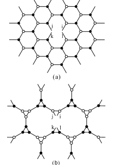
Figure 3: Configuration of an environment lattice (a) and that after one TRG iteration (b).

To understand this more clearly, let us rewrite the partition function (1) as

$$Z=\textrm{Tr}MM^{e}=\sum_{ij,kl}M_{ij,kl}M^{e}_{kl,ij},$$ (6)

where $M^{e}$ is the contribution from the environment lattice defined in Fig. 3. $M^{e}$ is defined by tracing out all bond indices in the environment lattice excluding those connecting with the two vertices on which $M$ is defined. This formula indicates that to reduce the error in $Z$, one needs to minimize the truncation error of $MM^{e}$, rather than that of $M$.

Fig. 3(a) shows the configuration of an environment lattice. In the rewiring and truncation of $M$-matrix, there is no need to evaluate $M^{e}$ rigourously. We propose to evaluate $M^{e}$ iteratively using the TRG method. The configuration of the environment after one TRG iteration before decimation is shown in Fig. 3(b). By contracting all the internal bonds connecting small triangles, a decimated environment lattice, whose configuration is similar to Fig. 3(a), is obtained. This iteration can be repeated until $M^{e}$ is converged. Generally we find that the values of $M^{e}$ such obtained are sufficiently accurate after 5 to 10 iterations, the corresponding numbers of environment lattice sites are $2\times 3^{5}-2$ and $2\times 3^{10}-2$, respectively.

 

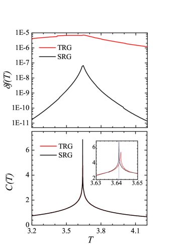
Figure 4: (color online) Comparison of the relative error of the free energy $\delta f(T)=|f(T)-f_{ex}(T)|/f_{ex}(T)$ (upper panel) and the specific heat (lower panel) as functions of temperature for the Ising model on triangular lattices obtained using TRG (red) and SRG. $f_{ex}(T)$ is the exact result calculated using the formula given in Ref. Wannier1950 . The dotted line in the Inset is the exact critical temperatures $T_{c}=4/\ln 3$

In the minimization of the truncation error of $MM^{e}$, it is better to treat the row $ij$ and column $kl$ indices of $M$ as symmetrically as possible. To do this, let us first do a singular value decomposition for $M^{e}$

$$M^{e}=U_{e}\Lambda_{e}V_{e}^{\dagger},$$ (7)

where $U_{e}$ and $V_{e}$ are two unitary matrices and $\Lambda_{e}$ is a semi-positive diagonal matrix. Then we can define a new matrix

$$\tilde{M}=\Lambda_{e}^{1/2}V_{e}^{\dagger}MU_{e}\Lambda_{e}^{1/2},$$ (8)

and show that

$$Z=\textrm{Tr}\tilde{M}.$$ (9)

Thus to minimize the error in $Z$, one needs only to minimize the truncation error of $\tilde{M}$.

Now let us take a singular value decompostion for $\tilde{M}$

$$\tilde{M}=\tilde{U}\tilde{\Lambda}\tilde{V}^{\dagger}.$$ (10)

Again, $\tilde{U}$ and $\tilde{V}$ are two unitary matrices. $\tilde{\Lambda}$ is a semi-positive diagonal matrix whose diagonal matrix elements are arranged in descending order. Then we can truncate the basis space by keeping the $D_{cut}$ largest singular values of $\tilde{\Lambda}$. By substituting the approximate $\tilde{M}$ back into Eq. (8), one can find that

$$M_{ij,kl}\approx\sum_{n=1}^{D_{cut}}S^{a}_{n,ij}S^{b}_{n,kl},$$ (11)

where

$$S^{a} = \tilde{\Lambda}^{1/2}\tilde{U}^{\dagger}\Lambda_{e}^{-1/2}V_{e}^{\dagger},$$ (12)

$$S^{b} = \tilde{\Lambda}^{1/2}\tilde{V}^{\dagger}\Lambda_{e}^{-1/2}U_{e}^{\dagger}$$ (13)

are the two tensors defined in the rewired lattice. Finally one can follow the steps introduced in Ref. Levin2007 to update tensors $T^{a}$ and $T^{b}$ in a squeezed lattice by taking the coarse grain decimation of $S^{a}$ and $S^{b}$. This completes a full cycle of SRG iteration. By repeating this procedure, one can finally obtain the value of partition function in the thermodynamic limit.

We have applied this SRG method to the spin-1/2 Ising model on triangular lattices. Fig. 4 compares the relative error of the free energy and the specific heat obtained using the SRG with those using the TRG. The number of sites is $3^{30}$ and $D_{cut}=24$. In the SRG calculation of $M^{e}$, 10 iterations are used. For the free energy, we find that the SRG can improve the accuracy for more than five orders of magnitude far away from the critical point, and more than two orders of magnitude at the critical point. The critical temperature $T_{c}$ can be determined from the peak position of the specific heat. As shown in the Inset of Fig. 4, the value of $T_{c}$ obtained with SRG is more than two orders of magnitude more accurate than that obtained with TRG. Furthermore, from our calculation, we find that the improvement of the SRG over the TRG becomes more and more pronounced with increasing $D_{cut}$.

It is straightforward to extend the SRG to study ground state properties of a quantum system with tensor-network wavefunction. The two-dimensional tensor-network wave function can be accurately determined using the projection approach we recently proposedJiang2008 . After that one can use the SRG to evaluate the expectation values of the tensor-network statenote .

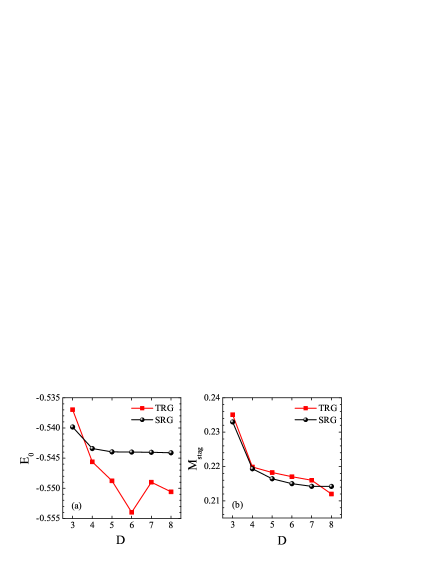
Figure 5: (color online) (a) The ground state energy per site $E_{0}$ and (b) the staggered magnetization $M_{stag}$ as functions of the bond degrees of freedom $D$ on honeycomb lattices.

To demonstrate how the SRG can improve the accuracy of the expectation values of tensor-network states, we have applied the SRG to the Heisenberg model on honeycomb lattices. The ground state wavefunction is assumed to have the following tensor-network form

$$|\Psi\rangle = \mathrm{Tr}\prod_{i\in b,j\in w}\lambda_{x_{i}}\lambda_{y_{i}}\lambda_{z_{i}}A_{x_{i}y_{i}z_{i}}[\sigma_{i}]B_{x_{j}y_{j}z_{i}}[\sigma_{j}]$$ (14)

$$|\sigma_{i}\sigma_{j}\rangle.$$

A schematic representation of this tensor-network state on the honeycomb lattice is shown in Fig. 1(b). $\sigma_{i}$ is the eigenvalue of spin operator $S_{iz}$. $A_{x_{i}y_{i}z_{i}}[\sigma_{i}]$ and $B_{x_{j}y_{j}z_{j}}[\sigma_{j}]$ are the two three-indexed tensors defined on the black and white sublattices, respectively. $\lambda_{\alpha_{i}}$ ($\alpha=x,y,z$) is a positive diagonal matrix of dimension $D$. The trace is to sum over all spin configurations and over all bond indices. The tensor corresponding to $T^{a}$ in Eq. (1) is now defined by

$$T^{a}_{xx^{\prime},yy^{\prime},zz^{\prime}} = \sum_{\sigma}(\lambda_{x}\lambda_{y}\lambda_{z})^{1/2}A_{xyz}[\sigma]$$

$$A_{x^{\prime}y^{\prime}z^{\prime}}[\sigma](\lambda_{x^{\prime}}\lambda_{y^{\prime}}\lambda_{z^{\prime}})^{1/2}.$$

The bond dimension of this tensor is $D^{2}$.

Fig. 5 compares the SRG with the TRG results for the ground state energy and the staggered magnetization for the Heisenberg model on the honeycomb lattice. The number of lattice sites is $2\times 3^{18}$. The truncation error in the SRG calculation is less than $\varepsilon_{0}\sim 10^{-3}$ and $D_{cut}=D^{2}$. We have used the second order Trotter-Suzuki decomposition formula to improve the accuracy in the calculation of the ground state wavefunctions using the projection approach introduced in Ref. Jiang2008 . The staggered magnetization is evaluated directly from the expectation value of the staggered spin operator in the ground state in the limit the external staggered magnetic field approaching zero. This avoids the error in the determination of the staggered magnetization from the numerical derivative of the ground state energy at finite staggered magnetic field, as was done in Ref. Jiang2008 . Unlike the TRG results, we find that the SRG results vary monotonically with $D$ and tend to converge quickly to the infinite $D$ limit.

For $D=8$, the SRG results of the ground energy and the staggered magnetization per site are respectively -0.5445 and 0.2142, consistent with the results obtained by other methodsZheng1991 ; Oitmaa1992 ; Reger1989 . The accuracy of these results are still not comparable with those obtained by the DMRGWhite07 and the quantum Monte Carlo methodSandvik . By considering the symmetry of the Hamiltonian, the tensor-network states with a bond dimension as large as $D\sim 20$ can in principle be handled. In that case, the SRG results will be further improved.

In conclusion, we have introduced a SRG method to improve significantly the accuracy in the TRG calculation. This method differs from the TRG by taking into account the renormalization effect of environment to the $M$-matrix, similar as the DMRG contrasting the conventional block renormalization group method. For the classical Ising model, the relative error of the free energy as well as other quantities is reduced by more than two to five orders of magnitude when $D_{cut}=24$ and can be further reduced by increasing $D_{cut}$, in comparison with the TRG. The SRG, in combined with the projection method introduced in Ref. Jiang2008 , provides an accurate and efficient tool for exploring tensor-network ground states of quantum lattice models. It will play a more and more important role in the study of highly correlated systems. The physical idea present in this work can be also generalized to apply to other physical problems where the system can be divided into two parts and the interplay between them is important. In particular, if one wants to generalize the projection method proposed in Ref. Jiang2008 to evaluate time-dependent or thermodynamic quantities, then the SRG correction to the wavefunction should be considered to minimize the accumulated Trotter and truncation errors in the iteration.

This work was supported by the NSF-China and the National Program for Basic Research of MOST, China.

References

- (1) H. Niggemann, A. Klümper, J. Zittartz, Z. Phys. B 104, 103 (1997).
- (2) F. Verstraete and J. Cirac, cond-mat/0407066.
- (3) M. Levin and C.P. Nave, Phys. Rev. Lett. 99, 120601 (2007).
- (4) H.C. Jiang, Z.Y. Weng, T. Xiang, Phys. Rev. Lett. 101, 090603 (2008).
- (5) Z.C. Gu, M. Levin, X.G. Wen, Phys. Rev. B 78, 205116 (2008).
- (6) S. stlund and S. Rommer, Phys. Rev. Lett. 75, 3537 (1995).
- (7) S.R. White, Phys. Rev. Lett. 69, 2863 (1992).
- (8) G.H. Wannier, Phys. Rev 79, 357 (1950); Phys. Rev. B 7, 5017 (1973).
- (9) The expectation value of a tensor-network state can be also determined using the transfer matrix renormalization group method. R.J. Bursill, T. Xiang, and G.A. Gehring, J. Phys.: Condens. Matt. 8, L583 (1996); X. Wang and T. Xiang, Phys. Rev. B 56, 5061 (1997).
- (10) W. Zheng, J. Oitmaa, and C.J. Hamer, Phys. Rev. B 44, 11869 (1991).
- (11) J. Otimaa, C.J. Hamer, and W. Zheng, Phys. Rev. B 45, 9834 (1992).
- (12) J.D. Reger, J.A. Riera, and A.P. Young, J. Phys.: Condens. Matter 1, 1855 (1989).
- (13) S.R. White and A.L. Chernyshev, Phys. Rev. Lett. 99, 127004 (2007).
- (14) A.W. Sandvik and H.G. Evertz, arXiv:0807.0682.