Quantum phase diagram of a spin-1/2 antiferromagnetic chain with magnetic impurity

Abstract

We present the renormalization group (RG) flow diagram of a spin-half antiferromagnetic chain with magnetic impurity and one altered link. In this two parameters (competing interactions) model, one can find the complex phase diagram with many interesting fixed points. There is no evidence of intermediate stable fixed point in weak coupling phase. It may arise at the strong coupling phase. Depending on the strength of couplings the phases correspond either to a decoupled spin with Curie law behavior or a logarithmically diverging impurity susceptibility as in the two channel Kondo problem.
Keywords: Spin Chain Model, Renormalization Group Methods
Pacs: 75.10.Pq, 05.10.Cc

I I. Introduction

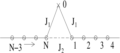
Figure 1: Schematic diagram of impurity model with two parameters, $J_{1}$ and $J_{2}$. Cross sign indicates the position of impurity and the circle represents the regular spin sites in the chain.

The physical behaviors of impurities in the low dimensional magnetic and electronic systems are interesting in their own right. There are few important studies in the literature to describe the behavior of different magnetic impurity configurations and defects in the antiferromagnetic Heisenberg spin chain aff1 ; egg1 ; egg2 ; egg3 . The chain with one altered link and two altered links are, respectively renormalized to an effective open boundary and periodic boundary conditions egg1 . We would like to revisit the problem of spin-1/2 antiferromagnetic chain with magnetic impurity and one altered link (Fig. 1). Motivation of this work comes from the considerable amount of debate on the RG flow diagram and the nature of the Fixed points of this problem egg3 ; zvy ; egg4 and also for the interesting physics of low dimensional spin systems dago . In this communication, we would like to resolve this debate through the numerical analysis of the RG equations and the stability analysis of the fixed point (FP). Before we proceed further, we would like to state the important results that have already existed in the literature of this field. An impurity spin s coupled to one site in the chain gets screened with a decoupled singlet of spin s- 1/2 and becomes an open chain with one site removed nag . An impurity spin coupled to two sites in the chain is equivalent to the two channel Kondo effect gia1 . Kondo effect in one dimension has developed based on the separation of charge and spin in the one dimensional electron gas. The single impurity Kondo effect only involves the spin degree of freedom of the one dimensional electron gas, the charge degrees of freedom are not playing the fundamental role in the Kondo effect nag . The spin degrees of freedom of the one-dimensional interacting electron system at low energies can be described as half-integer Heisenberg antiferromagnetic spin chain. Hence it is natural to look for a Kondo effect involving a magnetic impurity interacting with Heisenberg chain egg1 .

II II. Renormalization Group study of model Hamiltonian

We now present renormalization group (RG) study of two parameter model (${J_{1}},{J_{2}}$). The model Hamiltonian of our system is

$$H=J\sum_{i=1}^{N-1}\vec{S_{i}}.\vec{S_{i+1}}+J_{1}\vec{S_{0}}.(\vec{S_{N}}+\vec{S_{1}})+J_{2}\vec{S_{N}}.\vec{S_{1}}$$ (1)

$J$ is the nearest-neighbor Heisenberg exchange coupling. $J_{1}$, the symmetric coupling of the impurity to two sites in the chain and the coupling between two sites is $J_{2}$ (Fig. 1). At low temperature, this system is known to be well described by a level 1 Wess-Zumino-Witten model with a marginal irrelevant operator egg1 ; aff2 . A spin operator at the position x in the chain can be expressed in terms of current operators $\vec{J}$ and WZW field $g$,

$$\vec{{S_{j}}}(x)~{}=~{}\vec{J_{L}}~{}+~{}\vec{J_{R}}+constant*~{}{(-1)^{j}}tr[\vec{\sigma}g]$$ (2)

where $\vec{J_{L}}$ and $\vec{J_{R}}$ are the left and right SU(2) currents. ${J_{L}}(x)~{}=~{}-\frac{i}{4\sqrt{\pi}}tr[g^{\dagger}{{\partial}_{-}}g{\sigma}]$ ${J_{R}}(x)~{}=~{}\frac{i}{4\sqrt{\pi}}tr[{{\partial}_{+}}gg^{\dagger}{\sigma}]$. $g$ is related with the Abelian boson field $\phi$ and ${\tilde{\phi}}$ egg1 ; aff2 ,

$$g\propto\left(\begin{array}[]{cc}ie^{i\sqrt{2\pi}}{\phi}&e^{i\sqrt{2\pi}}{\tilde{\phi}}\\ -e^{-i\sqrt{2\pi}}{\tilde{\phi}}&-ie^{-i\sqrt{2\pi}}{\phi}\end{array}\right)$$

, where ${\phi}~{}=~{}{\phi}_{R}+{\phi}_{L}$ and $\tilde{{\phi}}~{}=~{}{\phi}_{R}-{\phi}_{L}$. This model Hamiltonian has already been studied by Eggert $et~{}al.$ egg3 ; egg4 by using field-theory arguments and numerical calculations. They have predicted the possibilities of different fixed points based on simple boundary conditions egg3 ; egg4 . Here we briefly describe those fixed points and their consequences in the phase diagram. (1). $P_{N+1}$: $J_{1}=J$ and $J_{2}=0$, a periodic chain with $N+1$ sites and no impurity spin. In this fixed point leading irrelevant operator is ${{\partial}_{x}}trg$ because the site parity symmetry does not allow more relevant operators. The authors of Ref. (egg4 ) conclude that this FP is stable in all directions of $J_{1}-J_{2}$ phase diagram egg3 ; egg4 . We will see in our study that there is no intermediate stable fixed point.

(2). $O_{N}$: $J_{1}=0$ and $J_{2}=0$, a periodic chain with N sites and a decouple impurity spin. The leading operator $(~{}\vec{J_{L}}(0)+\vec{J_{L}}(N)~{}).{\vec{S}}_{imp}$ of scaling dimension one is created by the coupling $J_{1}$ to the impurity from the open ends. This operator is marginally relevant for a antiferromagnetic coupling and irrelevant for ferromagnetic coupling. ${\vec{S}}_{imp}$ is the spin at the impurity site. ${J_{L}},{J_{R}}$ and $g$ have already defined in Eq. 2. The coupling between the end spins , $J_{2}$, can only produce the irrelevant operators egg3 ; egg4 .

(3). $O_{N-2}$: ${J_{1}}=0$ and ${J_{2}}\rightarrow\infty$, near this fixed point, impurity spin is separated by a locked singlet, which is effectively decoupled from the rest of the chain egg3 ; egg4 .

(4). $P_{N}$: $J_{1}=0$ and $J_{2}=J$, a periodic chain with N sites and a decoupled impurity spin. The most relevant operator $trg$ corresponds to a slight modification of one link in the chain $J_{2}$. A small coupling to the impurity spin $J_{1}$ produces the operator $(\vec{J_{L}}+\vec{J_{R}}).{\vec{S}}_{imp}$. The irrelevant operator ${{\partial}_{x}}tr({\vec{\sigma}}g)$ of dimension $d=3/2$ is also created by $J_{1}$ egg3 ; egg4 .

The author of Ref. zvy has argued that the analysis of the FPs of Ref. egg4 is not the complete one. There exist several other FPs like ${J_{1}}\rightarrow-\infty$ and ${J_{2}}\rightarrow-\infty$. He has argued at least one extra FP exist with $J_{1}\rightarrow\infty$.

The authors of Ref. egg3 ; egg4 , have expressed impurity Hamiltonian at the fixed point $P_{N}$ as

$$H_{imp}={{\gamma}_{1}}trg+{{\gamma}_{2}}(\vec{J_{L}}+\vec{J_{R}}).\vec{S_{imp}}+{{\gamma}_{3}}{{\partial}_{x}}tr(\vec{\sigma}g).\vec{S_{imp}},$$ (3)

where ${{\gamma}_{1}}\propto(J_{2}-J)$, ${{\gamma}_{2}}\propto J_{1}$ ${{\gamma}_{3}}\propto J_{1}$. ${J_{L}},{J_{R}}$ and $g$ have defined in Eq. 2. They have obtained the RG equations as follows

$$\frac{d{{\gamma}_{1}}}{dl}~{} = ~{}\frac{1}{2}{{\gamma}_{1}}~{}-~{}\frac{3}{2}{{\gamma}_{2}}{{\gamma}_{3}},$$

$$\frac{d{{\gamma}_{2}}}{dl}~{} = ~{}{{\gamma}_{2}}^{2}-\frac{3}{4}{{\gamma}_{3}}^{2},$$

$$\frac{d{{\gamma}_{3}}}{dl}~{} = ~{}-\frac{1}{2}{{\gamma}_{3}}+2{{\gamma}_{3}}{{\gamma}_{2}},$$

The third equation of the above RG equations has generated dynamically. We obtain the RG flow diagram by solving the above mentioned equations with sophisticated numerical package, MATLAB. These RG equations have both trivial, (${{\gamma}_{1}}^{*},{{\gamma}_{2}}^{*},{{\gamma}_{3}}^{*}$) = ($0,0,0$) and nontrivial fixed points (${{\gamma}_{1}}^{*},{{\gamma}_{2}}^{*},{{\gamma}_{3}}^{*}$) = ($\frac{\sqrt{3}}{8},\frac{1}{4},\frac{1}{2\sqrt{3}}$). We do the linear stability analysis to check the stability of these fixed points (FP). After the linear stability analysis RG equations reduce to

$$\frac{d}{dl}A_{1}~{}=~{}B_{1}A_{1},$$ (5)

where

$$A_{1}=\left(\begin{array}[]{c}{\gamma}_{1}\\ {\gamma}_{2}\\ {\gamma}_{3}\end{array}\right)$$

and

$$B_{1}=\left(\begin{array}[]{ccc}\frac{1}{2}&\frac{-3}{2}{{\gamma}_{3}}^{*}&\frac{-3}{2}{{\gamma}_{2}}^{*}\\ 0&2{{\gamma}_{2}}^{*}&\frac{-3}{2}{{\gamma}_{3}}^{*}\\ 0&2{{\gamma}_{3}}^{*}&\frac{-1}{2}+2{{\gamma}_{2}}^{*}\end{array}\right)$$

. At the trivial fixed point, $\frac{d{\gamma}_{1}}{dl}~{}=~{}\frac{{\gamma}_{1}}{2}$ and $\frac{d{\gamma}_{3}}{dl}~{}=~{}-\frac{{\gamma}_{3}}{2}$, $\frac{d{\gamma}_{2}}{dl}~{}=~{}0*{\gamma}_{2}$. The equation for ${\gamma}_{1}$ is unstable whereas the equation for ${\gamma}_{3}$ is stable. The equation for ${\gamma}_{2}$ is marginal. If we look at the next order term for the marginal case, i.e., $\frac{d{\gamma}_{2}}{dl}~{}=~{}a{{\gamma}_{2}}^{2}$ ($a>0$), we say that FP at ${\gamma}_{2}~{}=~{}0$ is stable on the $x<0$ side and unstable on the $x>0$ side.
We now present the stability analysis near to the nontrivial FPs. After the linear stability analysis RG equations reduce to

$$\frac{d}{dl}A_{2}~{}=~{}B_{2}A_{2},$$ (6)

where

$$A_{2}=\left(\begin{array}[]{c}{\gamma}_{1}\\ {\gamma}_{2}\\ {\gamma}_{3}\end{array}\right)$$

and

$$B_{2}=\left(\begin{array}[]{ccc}\frac{1}{2}&\frac{-\sqrt{3}}{4}&\frac{-3}{8}\\ 0&\frac{1}{2}&\frac{-\sqrt{3}}{4}\\ 0&\frac{1}{\sqrt{3}}&0\end{array}\right)$$

.

The eigenvalues of the matrix $B_{2}$ are (${{\lambda}_{1}},{{\lambda}_{2}},{{\lambda}_{3}})~{}=~{}(1/2,1/4+i\sqrt{3}/{4},1/4-i\sqrt{3}/{4}$ ). One of them is real and positive and the other two have imaginary parts , conjugated to each other but the real part is positive. Hence the system is in an unstable phase.
In Fig. 2, we present the RG flow diagram in ${{\gamma}_{1}}-{{\gamma}_{2}}$ plane, ${{\gamma}_{3}}=0$ as a initial parameter. We observe that here there is no intermediate nontrivial FPs for small values of coupling constants. The different coupling constants are flowing off to the higher values at the different sector of RG flow diagram and the corresponding instabilities are growing up in the systems. In our RG flow diagram, once the coupling constants flowing off to the higher values, there is no opportunity to return in the weak coupling phase. So the system flowing off to the strong coupling phase. We conject about the existence of these strong coupling phases following the prescription of seminal work of Furusaki and Nagaosa on one dimensional Kondo problem nag , which is well accepted in the literature. They have had tentatively extended the scaling equation to the strong coupling region. One is ${{\gamma}_{1}}\rightarrow\infty$ (we denote this phase region by A), the effective coupling $J_{2}$ increases quickly so that two end spins lock into a singlet, upto a critical value of $J_{1}$. In region A, system flows to the $O_{N-2}$. The region B is the another strong coupling phase region, system flows to the $O_{N}$. In this phase region effective coupling, ${J_{2}}$ decreases to zero. The phase regions, A and B, are upto a critical value of $J_{1}$. When $J_{1}$ exceed the critical value, system drives to a another critical region C. This region is another strong coupling phase region, independent on the initial value of $J_{2}$. We call this fixed point as $O_{N+1}$, this FP appears at ${{\gamma}_{1}}=0$, i.e., ${J_{2}}=J$ and ${J_{1}}\rightarrow\infty$. This fixed point may coincide with the $P_{N+1}$ of Ref. egg3 ; egg4 for large values of $J_{1}$. There is no evidence of intermediate stable fixed point as claimed in Ref. [4-5]. There is no stability analysis of FPs in Ref. [4-6], hence the conjecture regarding the FPs are not consistent ones. In this strong coupling regime, impurity spin tightly bound to the nearest-neighbor spin and the system behaves like a two channel Kondo problem with logarithmic susceptibility. This FP occurs at $J_{2}=J$, so there is no opportunity that impurity spin and two neighboring spins decoupled from the chain. This conjecture is consistent with the findings of Ref. egg4 . So in this complex phase diagram, there is only one FP, ${O}_{N-2}$, where the spin singlet locked and decouple from the rest of the chain. In Ref. egg4 , performed the TMRG calculation to predict the parabolic phase boundary between the phases $O_{N}$ and $O_{N-2}$. The phase boundaries of our study is also parabolic. Our RG flow diagram is the extensive one . The phase regions A and B behave as a Curie law behavior as $T\rightarrow 0$ from the decoupled impurity spin degrees of freedom and region C is logarithmically divergent impurity susceptibility gia1 .
In. Fig. 3, we present the RG flow diagram in ${\gamma}_{1}$ - ${\gamma}_{2}$ plane, ${{\gamma}_{3}}=0.1$ is the initial parameter of the system. We observe only two strong coupling phases, ${O_{N-2}}$ and ${O_{N}}$. Most of the regions of the phase diagram corresponds to the B phase.
Similarly in Fig. 4, ${{\gamma}_{3}}=-0.1$ is the initial parameter of the system, here we also observe two strong coupling phase regions like Fig. 3 but most of the phase regions covers by the phase A. The studies of the effect of the initial values of ${\gamma}_{3}$ are absent in the previous studies egg3 ; zvy ; egg4 . There is no evidence of the existence of phase region C.

III III. Conclusions

We have revisited the problem of magnetic impurity in a spin-1/2 antiferromagnetic chain with one alter link. The phase diagram of the previous studies egg3 ; zvy ; egg4 are the schematic ones and there are no sound numerical analyses to predict the different fixed points and their nature (stability analysis of the fixed points). We have presented an extensive RG flow diagram and has also done the stability analysis of the FPs. We have predicted that there is no evidence of intermediate stable FPs at the weak coupling limit, i.e., for the small values of coupling constants. FP may arise for the large values of coupling constant (${J_{1}}$). We have concluded that this fixed point does not correspond to any completely decoupled phase. We have studied the explicit role of ${\gamma}_{3}$ term. For ${{\gamma}_{3}}=\pm 0.1$, our RG flow diagrams study is entirely new, the system possessing only two strong coupling phase regions.

Acknowledgments

The author would like to acknowledge The Center for Condensed Matter Theory of the Physics Department of IISc for providing working space and also Mr. M. Vasudeva for reading the manuscript very critically.

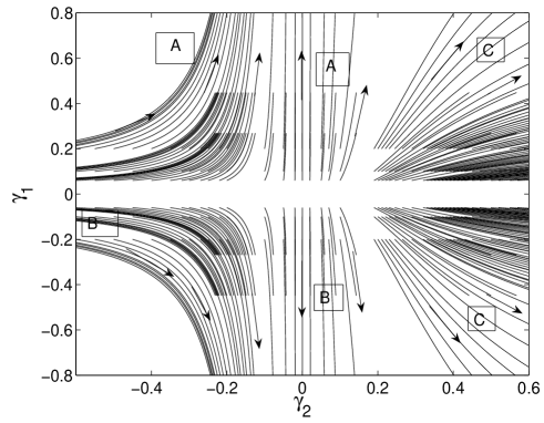
Figure 2: The RG flow diagram in the ${\gamma}1-{\gamma}2$ plane for Eq. 4 . The solid line and arrow show the flow and the direction respectively. This phase diagram consists of three strong coupling phase regions A ($O_{N-2}$), B ($O_{N}$) and C ($O_{N+1}$) (please see text for detailed analysis). ${\gamma}3=0$.

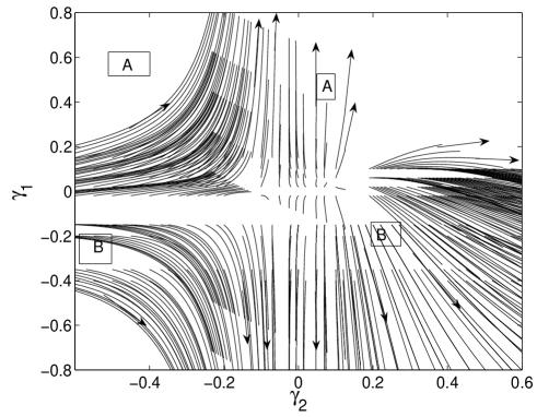
Figure 3: The RG flow diagram in the ${\gamma}1-{\gamma}2$ plane for Eq. 4. The solid line and arrow show the flow and the direction respectively. This phase diagram consists of two strong coupling phase regions A ($O_{N-2}$) and B ($O_{N}$) (please see text for detailed analysis). ${\gamma}3=0.1$.

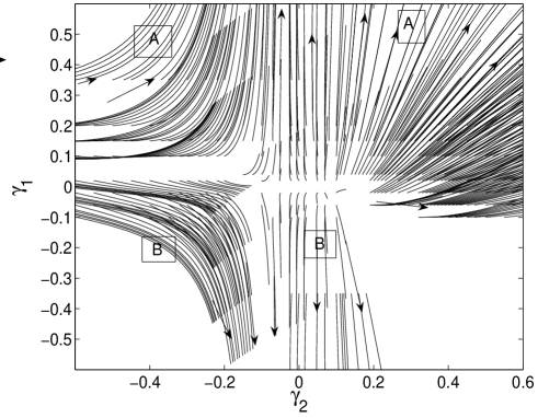
Figure 4: The RG flow diagram in the ${\gamma}1-{\gamma}2$ plane for Eq. 4 . The solid line and arrow show the flow and the direction respectively. This phase diagram consists of two strong coupling phase regions A ($O_{N-2}$) and B ($O_{N}$) (please see text for detailed analysis). ${\gamma}3=-0.1$.

References

- (1) I. Affleck, cond-mat/9311054; Acta Phys. Pol. B 26, (1995) 1869.
- (2) S. Eggert and I. Affleck, Phys. Rev. B 46, (1992) 10866.
- (3) S. Eggert and S. Rommer, Phys. Rev. Lett. 81, (1998) 1690.
- (4) S. Eggert, D. P. Gustafsson, and S. Rommer, Phys. Rev. Lett. 86, (2001) 516.
- (5) A. A. Zvyagin, Phys. Rev. Lett 87, (2001) 59701.
- (6) S. Eggert, D. P. Gustafsson and S. Rommer, Phys. Rev. Lett 87, (2001) 59702.
- (7) E. Dagato and T. M. Rice, Science 271, 618 (1996).
- (8) A. Furusaki and N. Nagaosa, Phys. Rev. Lett 72, (1994) 892.
- (9) D. G. Clarke, T. Giamarchi and B. I. Shariman, Phys. Rev. B 48, (1993) 7070.
- (10) I. Affleck, Fields Strings and Critical Phenomena, edited by E. Brezin and J. Zinn-Justin (North-Holland, Amsterdam, 1990), P. 563.