Brown-HET-1563

Remarks on Power Spectra of Chaotic Dynamical Systems

G. Guralnik, Z. Guralnik, C. Pehlevan

Department of Physics

Brown University

Providence, RI 02912

Abstract

We develop novel methods to compute auto-correlation functions, or power spectral densities, for chaotic dynamical systems generated by an inverse method whose starting point is an invariant distribution and a two-form. In general, the inverse method makes some aspects of chaotic dynamics calculable by methods familiar in quantum field theory. This approach has the numerical advantage of being amenable to Monte-Carlo parallel computation. We demonstrate the approach on a specific example, and show how auto-correlation functions can be computed without any direct numerical simulation, by Pade approximants of a short time expansion.

1 Introduction

Due to their sensitive dependence on initial conditions, the precise behavior of a chaotic dynamical system over long times is unpredictable in practice, even though the underlying system is deterministic. However there is no fundamental obstruction to calculating statistical properties of the long time behavior of chaotic systems.

Typically, statistical properties of chaotic systems are calculated by direct numerical simulation, with the assumption that the statistics, in the form of time averages, converge quickly compared to the rate at which numerical errors accumulate due to the sensitivity to initial conditions. Direct numerical simulation of systems with a very large number of degrees of freedom requires significant computational power which in many cases is not yet available. Moreover, it is difficult to gain theoretical insight from direct simulations.

In a previous paper [1], which we review in section II, we described an alternative approach to direct numerical simulation. This approach involves an inverse method whereby chaotic dynamical systems are generated, given a two-form and exact statistical information given by an invariant distribution over phase space. Several examples of chaotic systems were given for which there was precise agreement between equal time moments calculated by direct numerical simulation or by using the initial invariant distribution.

There are several advantages to the inverse approach over direct simulation. In principle, the inverse approach can be applied to systems with a large number of degrees of freedom, without placing intense demands on computational power. It is also possible to begin a classification of chaotic systems in terms of analytic properties of the statistics. We expect that, using the inverse approach, many theoretical insights into properties of chaotic dynamical systems are forthcoming.

In [1], only equal time moments (and cumulants) were computed for chaotic systems generated by the inverse approach. The present work is a sequel to [1], in which we will apply the inverse method to the computation of auto-correlation functions, whose Fourier transform is the power spectral density. Ordinarily, the auto-correlation or power spectrum is computed by a direct numerical simulation with a long run-time. However, for chaotic systems generated by the inverse method, the auto-correlation can be computed by a Monte-Carlo simulation, involving many fixed time simulations from different initial conditions, as opposed to one long simulation. This has the great advantage of being amenable to parallel computation. We discuss the Monte-Carlo approach in section III. Although we only consider auto-correlation functions here, we emphasize that our approach is applicable to any correlation functions of phase space variables at different times.

For chaotic systems generated by the inverse method, it is also possible to calculate auto-correlation functions without direct numerical simulation. In section IV, we show that the inverse approach yields a small $t$ expansion for the auto-correlation $G(t)$, whose validity can be extended deeper into the complex $t$ plane by Pade approximants. We shall see that this approach shows good agreement with results obtained by direct numerical simulation.

Power spectra of dynamical systems are sometimes obtained from Fourier decomposition of a signal within some time window. For a chaotic system, this approach is rife with ambiguities and pitfalls, unlike the Fourier transform of the auto-correlation function which is well defined. However these pitfalls are themselves interesting and can be well understood using the inverse approach, as we shall see in section V.

2 Review of the inverse approach

We give a very brief review of the inverse method here. For details the reader is referred to [1]. We consider deterministic dynamical systems, with phase space coordinates $x_{1}(t)\cdots x_{N}(t)$ and equations of motion

$$\frac{dx_{n}}{dt}=v_{n}(x_{1},\cdots x_{N})$$ (2.1)

A distribution over initial conditions $\rho[x]$ which is left invariant by the time evolution is a solution of the zero diffusion limit of the static Fokker-Planck equation,

$$\vec{\nabla}\cdot(\rho\vec{v})=0\,,$$ (2.2)

For $N=3$, this implies that $\rho\vec{v}$ can be written as the curl of a vector field,

$$\vec{v}=\frac{\vec{\nabla}\times\vec{A}}{\rho}\,,$$ (2.3)

and the inverse method amounts to choosing $\vec{A}$ and $\rho$, such that $\vec{v}$ is polynomial in the phase space coordinates $x_{n}$. For $N>3$, it is convenient to use the language of differential forms, in which case (2.1) becomes

$$d{}^{*}(\rho v)=0$$ (2.4)

where $v$ is the velocity one form $v_{m}dx^{m}$, $d$ is the exterior derivative, and * indicates the Hodge dual. This implies that

$$v=\frac{{}^{*}d{\cal A}}{\rho}$$ (2.5)

where ${\cal A}$ is an $N-2$ form. The problem is then to choose $\rho$ and ${\cal A}$ such that $v$ is polynomial in $x_{n}$. This was done in [1] for a few increasingly complex analytic structures of $\rho$ and ${\cal A}$.

Since ${}^{*}{\cal A}$ is a two-form, which is more conveniently written down for large $N$ than ${\cal A}$, it can be said that an invariant distribution and a two-form uniquely specify dynamical systems. This is very similar to the specification of Hamiltonian dynamical systems by a Hamiltonian and a symplectic form, although far more general. For example $N$ need not be even, and a Liouville theorem, $d{}^{*}v=0$, need not apply. There also are not necessarily any conserved quantities.

Amongst the simplest distributions, so far as analytic structure is concerned, are polynomial distributions for which the real zeroes form a closed manifold inside of which the polynomial is positive. For these,

$${\cal A}=\rho^{2}\Omega$$ (2.6)

were $\rho$ is a polynomial, and $\Omega$ is a polynomial $N-2$ form, so that

$$v={}^{*}(\rho d\Omega+2d\rho\wedge\Omega)$$ (2.7)

Chaotic dynamical systems of this type are invariably repellers (see [1]). Chaotic attractors arise from distributions and two-forms with more complicated analytic structure, which are also discussed in [1].

Although a distribution $\rho$ satisfying (2.1) is an invariant distribution over initial conditions, it does not necessarily describe the statistics of a single chaotic trajectory. It must be verified that the dynamics is chaotic and that $\rho$, or strictly speaking its projection, is an ergodic measure, having no convex decomposition into independent invariant measures $\rho\neq x\rho_{1}+(1-x)\rho_{2}$. In many instances it is necessary to modify the domain of support of the initial distribution $\rho$ to make it ergodic. For chaotic invariant sets with fractional information dimension, a function $\rho(x)$, with support in $N$ dimensions, can not be ergodic, although it may still contain exact information about the statistics, either via projection to lower integer dimension or, after Fourier transformation, as the generator of polynomial moments. The question of the general relevance of the distributions $\rho$ arising in the inverse approach has not been definitively resolved. However, for the chaotic systems which have been considered so far in [1], the distributions used to generate the dynamical systems give extremely accurate results for moments and cumulants (connected equal time correlation functions). Of course it is possible that these systems have information dimension which is very nearly $N$, in which case $\rho$ yields, at worst, an extremely accurate approximation to the exact statistics.

We emphasize that the results in this article are not restricted to chaotic dynamical systems generated by the inverse method. In fact, they may be applied to any system for which there is known information about the invariant measure over phase space or equal time moments. The point of this article is to use known information about static (time independent) statistics to facilitate the computation of time dependent quantities, such as auto-correlation functions and power spectral densities.

3 Monte-Carlo computation of the auto-correlation and power spectrum

Power spectra are useful signatures of dynamical systems derived from time series data. The power spectrum associated with a signal $x(t)$ is defined as the squared amplitude of the Fourier transform of $x(t)$. However, the Fourier transform of an a-periodic chaotic signal $x(t)$ is not generally well defined since $x(t)$ does not fall of as $t\rightarrow\pm\infty$. The power spectral density on the other hand is well defined;

$$\tilde{G}(\omega)\equiv\int_{-\infty}^{\infty}\,d\Delta\,\exp(i\omega\Delta)G(\Delta)$$ (3.8)

where $G(\Delta)$ is the auto-correlation function,

$$G(\Delta)\equiv\lim_{T\rightarrow\infty}\frac{1}{T}\int_{-T/2}^{T/2}\,dt\,x(t)x(t+\Delta)\,.$$ (3.9)

Due to the tendency of chaotic systems to ‘forget’ their initial conditions, $G(\Delta)$ falls off with large $\Delta$ (assuming $<x>=0$) sufficiently rapidly that the Fourier transform (3.8) is well defined. The total power between frequencies $\omega$ and $\omega+d\omega$ is given by $\tilde{G}(\omega)d\omega$.

A remarkable property of chaotic systems is that time averages of functions of phases space over a trajectory are equal to spatial averages with respect to an ergodic measure:

$$<f>=\lim_{T\rightarrow\infty}\frac{1}{T}\int_{0}^{T}\,dt\,f(\vec{x}(t))=\int d\mu(\vec{X})f(\vec{X})$$ (3.10)

The auto-correlation of a phase space variable $x_{i}$ can therefore be written as

$$G_{i}(\Delta)=\int d\mu(\vec{X})f_{\Delta}(\vec{X})$$ (3.11)

where

$$f_{\Delta}(\vec{X})\equiv x_{i}(t=0)x_{i}(t=\Delta)\,,\,\,\,\,\,{\rm with}\,\,x_{i}(0)=X_{i}\,.$$ (3.12)

Thus, when the exact invariant measure is known, the auto-correlation and power spectral density can be computed by Monte-Carlo methods, which entail multiple fixed time simulations of the dynamical system from randomly generated initial conditions rather than a single very long simulation. This approach is amenable to efficient parallel computation schemes.

4 An example

Consider a specific chaotic system of the type (2.7) (studied in [1]) with

$$\rho =1-x^{4}-y^{2}-z^{6}$$

$$\Omega =(xyz)dy+(y^{2})dz\,.$$ (4.13)

yielding

$$v_{x}=13z^{6}xy-6y^{3}-xy+2y+yx^{5}-2yx^{4}-2yz^{6}+y^{3}x\,,$$

$$v_{y}=8x^{3}y^{2}\,,$$ (4.14)

$$v_{z}=-9x^{4}yz+yz-yz^{7}-y^{3}z\,.$$

Initial conditions with $\rho(x,y,z)>0$, $y>0$ and $z>0$ give rise to chaotic trajectories whose statistics are described by an invariant distribution $\tilde{\rho}=\rho$ for $\rho(x,y,z)>0,\,y>0,\,z>0$, up to a normalization, and $\tilde{\rho}=0$ outside this domain.

Next we will evaluate the auto-correlation $G_{x}(\Delta)=<x(t)x(t+\Delta)>$ for these chaotic trajectories. The auto-correlation can be evaluated by direct numerical simulation, taking the time average of $x(t)x(t+\Delta)$ over a long run-time. Alternatively, it can be evaluated using (3.11),(3.12);

$$G_{x}(\Delta)=\int dXdYdZ\tilde{\,}\tilde{\rho}(X,Y,Z)\,f_{\Delta}(X,Y,Z)$$ (4.15)

where

$$F_{\Delta}(X,Y,Z)=x(t=0)x(t=\Delta)$$ (4.16)

with

$$x(t=0)=X,\,\,y(t=0)=Y,\,\,z(t=0)=Z$$ (4.17)

Evaluating (4.15) by Monte Carlo simulation amounts to generating initial conditions $X,Y,Z$ randomly according to the distribution $\tilde{\rho}$, and simulating the time evolution from each of these points over a duration $\Delta$. The results of both the Monte-Carlo calculation and a direct long-duration numerical simulation of (4) are shown in figure 1, showing extremely good agreement.

The example we have given is a small dimension system, with $N=3$, so there is little computational advantage to the Monte-Carlo approach over a direct long duration simulation. The advantage comes at large $N$, for which the Monte-Carlo approach will be far faster, as it is amenable to parallel computation.

  

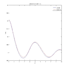
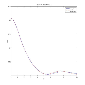
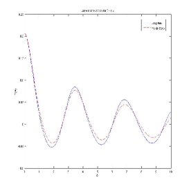
Figure 1: Auto-correlation functions calculated by Monte-Carlo simulation (dashed line) and direct long-duration simulation (solid line). The dimensionless number $\beta$ parameterizes a variation of the dynamical system (4), obtained from $\rho=1-x^{4}-y^{2}-z^{6},\,\,\,\Omega=(xyz)dy+\beta(y^{2})dz$.

5 Calculating the auto-correlation without direct
numerical simulation.

Using (3.11), the auto-correlation function $G_{i}(\Delta)$ can be expanded as a power series in $\Delta$. To do so let us first expand (3.12) in $\Delta$:

$$F_{\Delta}(\vec{X})\sim x_{i}(0)\left(x_{i}(0)+\Delta\dot{x}_{i}(0)+\frac{1}{2}\Delta^{2}\ddot{x}_{i}(0)\cdots\right)\,,\,\,\,{\rm with}\,\,\,\vec{x}(0)=\vec{X}\,.$$ (5.18)

Note that $x_{i}\frac{d^{n}x_{i}}{dt^{n}}$ can be written as a total time derivative for odd $n$:

$$x_{i}\frac{dx_{i}}{dt}=\frac{d}{dt}\left(\frac{1}{2}x_{i}^{2}\right),\,\,\,x_{i}\frac{d^{3}x_{i}}{dt^{3}}=\frac{d}{dt}\left(x_{i}\frac{d^{2}x_{i}}{dt^{2}}-\frac{1}{2}\left(\frac{dx_{i}}{dt}\right)^{2}\right)\,,\,\,{\rm etc}$$ (5.19)

For even $n$, $n=2m$,

$$x_{i}\frac{d^{n}x_{i}}{dt^{n}}=\frac{d}{dt}\left(g_{n}\right)+(-1)^{m}\left(\frac{d^{m}x_{i}}{dt^{m}}\right)^{2}$$ (5.20)

where we will not bother to specify $g_{n}$, since total time derivatives vanish when averaged over a chaotic trajectory. Thus

$$G(\Delta)=\left<F_{\Delta}\right>\sim\sum_{m=0}^{\infty}\alpha_{m}\Delta^{2m}$$ (5.21)

$$\alpha_{m}\equiv(-1)^{m}\frac{1}{2m!}\left<\left(\frac{d^{m}x_{i}}{dt^{m}}\right)^{2}\right>$$ (5.22)

Using the equations of motion

$$\frac{dx_{i}}{dt}=v_{i}(\vec{x})$$

the terms $(d/dt)^{m}x_{i}$ can be related to functions on phase space. For example

$$\frac{d^{2}x_{i}}{dt^{2}}=\frac{dv_{i}}{dt}=\sum_{j}v_{j}(\vec{x})\frac{\partial v_{i}(\vec{x})}{\partial x_{j}}$$

so that

$$\alpha_{2}=\left<\left(\frac{d^{2}x_{i}}{dt^{2}}\right)^{2}\right>=\int d\mu(\vec{X})\left(\sum_{j}v_{j}(\vec{X})\frac{\partial v_{i}(\vec{X})}{\partial X_{j}}\right)^{2}$$

Since $F_{\Delta}(\vec{X})$ can not have singularities on the real axis (the real solutions of the equations of motion are assumed to be non-singular), the series (5.21) has a finite radius of convergence. We propose to evaluate $G(\Delta)$ by Monte-Carlo integration to evaluate the coefficients $\alpha_{m}$, followed by a Pade resummation of (5.21).

For the dynamical system (4), the moments $\alpha_{m}$ are evaluated with respect to the measure $d\mu(\vec{x})=dxdydz\tilde{\rho}(\vec{x})$

$$\tilde{\rho}=1-x^{4}-y^{2}-z^{6}\,\,{\rm for}\,\,x^{4}+y^{2}+z^{6}<1\,,$$

$$\tilde{\rho}=0\,\,{\rm for}\,\,x^{4}+y^{2}+z^{6}\geq 1\,,$$ (5.23)

We have calculated $\alpha_{0}\cdots\alpha_{8}$ for the auto-correlation $G_{x}(\Delta)$ using Monte-Carlo simulation, together with a significant amount of algebra which was also carried out with a computer. The corresponding $(4|4)$ Pade approximant is a ratio of polynomials of degree 4 whose first 9 Taylor-Mclaurin series coefficients are $\alpha_{0}\cdots\alpha_{8}$. The $(4|4)$ Pade approximant to $G(\Delta)$ is plotted in figure 2, along with the 9’th order Taylor Mclauren series result and the result of direct numerical simulation by a long run of the dynamical system. Note that the 9-th order Taylor-Mclaurin series begins to differ markedly from the result of direct numerical simultation at $\Delta\sim 0.35$, well before the first zero, whereas the $(4|4)$ Pade approximant gives accurate result for much larger values of $\Delta$, and is an acceptable approximation up to a neighborhood of the first zero, $\Delta\sim 2$. Higher order Pade approximants are needed to obtain more real zeros, and to provide a good approximation of the exact result for larger values of $\Delta$. This requires more computing power than we have presently applied to the problem. Nevertheless, the initial results are very encouraging, suggesting that the auto-correlation may be computed without a direct simulation of the dynamical system.

  

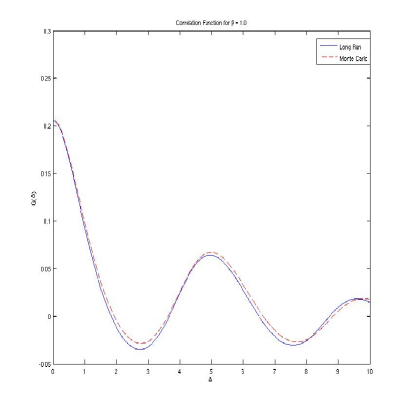
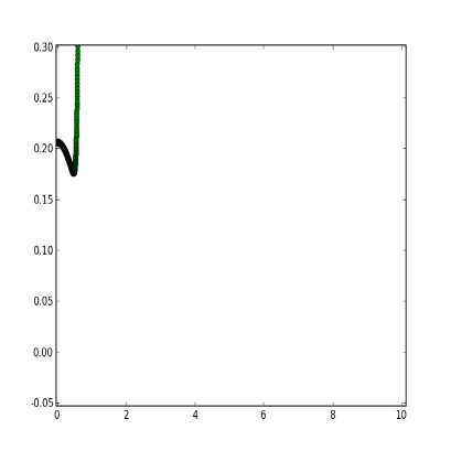
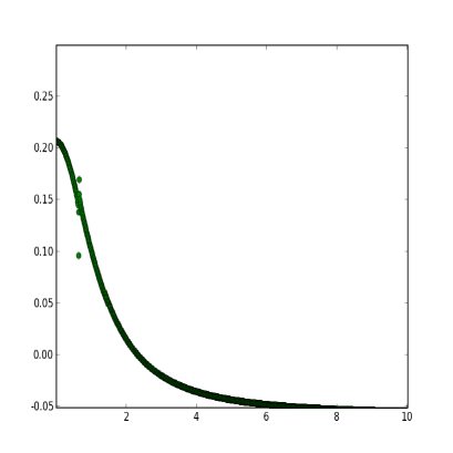
Figure 2: The auto-correlation calculated by long-run numerical simulation and by Monte-Carlo short run simulations (top), by 9’th order Monte-Carlo/Taylor-Mclauren series (bottom left) , and by Monte-Carlo/$(4|4)$ Pade approximant (bottom right). The Pade result is a smooth continuous curve, with the exception of a very small neighborhood of the point $\Delta=0.6529$, at which there is a spurious pole.

An oft stated property of chaotic power spectra is that there is non-zero exponentially small component at high frequency [3, 2], $\tilde{G}(\omega)\sim\exp(-\alpha\omega)$. The time-scale $\alpha$ is determined by the proximity of the nearest singularity of the auto-correlation $G(\Delta)$ to the real $\Delta$ axis. Note that there can not be any singularities on the real $\Delta$ axis, as it is assumed that the time evolution of the dynamical system does not encounter any singularities. Due to the tendency of chaotic systems to ‘forget’ their intial conditions, one expects singularities of $G(\Delta)$ near the real axis to occur for small values of $Re(\Delta)$. This suggest that the high frequency behavior of the power spectral density can be extracted from the small $\Delta$ behavior of the auto-correlation.

It may be possible to use the Pade approximant to the auto-correlation to get an estimate of the parameter $\alpha$. The poles of the Pade approximant do not necessarily correspond to the true analytic structure, and may in general be spurious. In fact the $(4|4)$ Pade approximant we have computed here has two poles which are likely spurious, including one on the positive real axis which is definitely spurious. These poles are extremely close to zeros of the Pade approximant. There is one pole which is not near any zero, at $\Delta=1.24i$. Verifying that this yields a good first approximation to $\alpha$ requires consideration of higher orders in the Pade sequence, $(n|n)$ for $n>4$, which we have yet to attempt.

6 Remarks on the Fourier transform of a chaotic signal

The Fourier transform of a chaotic trajectory $x(t)$,

$${\tilde{x}_{i}}(\omega)=\lim_{\epsilon\rightarrow 0}\int_{-\infty}^{\infty}\,dt\,e^{i\omega t}x_{i}(t)\,.$$ (6.24)

is not well defined. Nevertheless, it is quite common to take the Fourier (or discrete Fourier) transform of chaotic time series with some window of fixed duration, squaring the amplitude to give a kind of power spectrum.

Let us consider a function on phase space $f_{\omega}(\vec{X})$, defined by

$$f_{\omega}(\vec{X})=\frac{\omega}{2\pi}\int_{0}^{2\pi/\omega}dt\,x_{i}(t)e^{-i\omega t}$$ (6.25)

where

$$\vec{x}(t=0)=\vec{X}$$ (6.26)

and $\vec{x}(t)$ satisfies the equations of motion. Next consider a chaotic trajectory $\vec{X}(t)$, and define $<f_{\omega}>$ to be the time averaged value of $f_{\omega}(\vec{X}(t))$ on this trajectory. The average can be computed by summing over values of $f_{\omega}(\vec{X}(t))$ at arbitrary regular time intervals $\Delta t$, yielding a result which is independent of the interval. If one chooses the interval $\Delta t=2\pi/\omega$, one arrives at the formal result

$$<f_{\omega}>=\lim_{T\rightarrow\infty}\frac{1}{T}\int_{0}^{T}\,dt\,e^{-i\omega t}x_{i}(t)$$ (6.27)

In terms of the invariant measure $d\mu(\vec{X})$ on the phase space of a chaotic system, ergodicity implies

$$<f_{\omega}>=\int d\mu(\vec{X})f_{\omega}(\vec{X})$$ (6.28)

Note that different initial conditions $\vec{x}(0)$ which are different points on the same chaotic trajectory lead to a different overall phase in (6.27). On the other hand, (6.28), too which (6.27) is formally equivalent, has no reference to an initial condition. This is consistent only if $<f_{\omega}>=0$.

It is interesting to try to compute (6.28) by Monte-Carlo simulation. Note that any non-zero result is pure error, which we shall see is closely related to the power spectral density. The Monte-Carlo calculation amounts to generating a set of $n$ initial conditions randomly, according to the distribution of the chaotic invariant set, and then running the dynamical system from each initial condition for a duration $2\pi/\omega$. Given the chaotic ‘loss of information’ about initial conditions with time, one expects this to yield a very similar result to direct numerical simulation from a single initial condition over a duration $2\pi n/\omega$.

Calculating $<f_{\omega}>$ by Monte-Carlo simulation, any non-zero result is pure error, the size of which is related to the variance of $f_{\omega}$. The variance of $f_{\omega}$ can be expressed in terms of the auto-correlation,

$$<|f_{\omega}-<f_{\omega}>|^{2}> =\int_{0}^{2\pi/\omega}dt\int_{0}^{2\pi/\omega}dt^{\prime}\int d\mu(\vec{X})x(t)x(t^{\prime})e^{i\omega(t-t^{\prime})}$$ (6.29)

$$\vec{x}(t=0) =\vec{X}$$ (6.30)

so that

$$<|f_{\omega}-<f_{\omega}>|^{2}>=\int_{0}^{2\pi/\omega}dt\int_{0}^{2\pi/\omega}dt^{\prime}G(t-t^{\prime})e^{i\omega(t-t^{\prime})}$$ (6.31)

Note that (6.31) is very similar to the power spectral density, with the exception of the boundaries of integration.

We have calculated a ‘power spectrum’ for the dynamical system defined by (4), defined as the square of the amplitude of a discrete Fourier transform within some time window, or of a Monte-Carlo approximation to $f_{\omega}$. The results of both calculations for $\beta=1$ are plotted in figure 3.

  

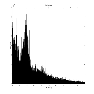
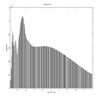
Figure 3: ‘Power spectrum’ computed by Fast Fourier Transform of a chaotic signal (on the left) and by Monte-Carlo simulation (on the right).

Due to the tendency of chaotic systems to ‘forget’ their initial conditions, on might expect the Fourier transform of a run of finite but long duration to be qualitatively similar to the Monte-Carlo result, which involves shorter runs from randomly generated initial conditions. Indeed the results plotted in figure 3 have some crude qualitative equivalence. In some sense, both these results can be viewed as nothing but finite total simulation time errors, the exact result vanishing identically, where the error is related to a quantity (6.31) similar, but not equivalent, to the power spectral density.

7 Conclusions

Direct numerical simulation of chaotic dynamical systems is a viable method to compute their statistics. However this approach rarely yields theoretical insight, and places extreme or prohibitive demands on computational resources for systems with a very large number of degrees of freedom. The intent of this work has been to develop an inverse method, introduced in [1], which permits the calculation of statistical quantities of chaotic systems without the use of direct numerical simulation over long time durations.

The inverse method generates chaotic dynamical systems, given an invariant measure and a two-form. At present we we have tested the approach on systems with a small number of degrees of freedom, by computing static statistical quantities in [1] such as equal time correlations, and time dependent statistical quantities such as auto-correlation functions in the present article.

Already at the level of a few degrees of freedom, one should be able to make theoretical progress which is not possible with studies involving only direct numerical simulation. In particular it should be possible to construct a classification of chaotic dynamical systems according to the phase space analytic structure of an invariant distribution and a two-form.

Given the invariant measure of a chaotic dynamical system, which is the starting point of the inverse approach, one can write closed form expressions for equal time correlation functions, for which analytic approximation schemes may exist, such as saddle point expansions. Non-equal time correlation functions, such as auto-correlations, may also be computable without recourse to direct numerical simulation, by Pade re-summation of short time expansions. In fact, many of the calculations arising using the inverse approach bear a close resemblance to calculations in quantum field theory, which may yield useful ideas in the present context of chaotic dynamics.

The true power of the inverse method will come for a large number of degrees of freedom, since this approach is amenable to parallel computation. There are numerous interesting problems which remain to be solved, in particular that of reverse engineering a chaotic dynamical system of particular physical interest, such as a turbulent fluid. Efforts along these lines are underway.

There remain subtle and interesting theoretical problems concerning the meaning of the invariant distribution, which is the starting point of the inverse method, when the information dimension is fractional. These subtleties have been discussed in [1] and remain to be resolved.

8 Acknowledgments

We wish to think S. Libby for helpful discussions. The work of G. Guralnik and C. Pehlevan is supported in part by funds provided by the U.S. Department of Energy (DoE) under DE-FG02- 91ER40688-Task D.

References

- [1] Z. Guralnik, Exact statistics of chaotic dynamical systems, arXiv.org:0804.3793
- [2] D. Sigeti, Exponential decay of power spectra at high frequency and positive Lyapunov exponents, Physica D 82 (1995) 136-153.
- [3] U. Frisch and R. Morf, Intermittency in nonlinear dynamics and singularities at complex times, Phys. Rev. A 23 ( 1981) 2673-2705.