Solitons in one-dimensional photonic crystals

Abstract

We report results of a systematic analysis of spatial solitons in the model of 1D photonic crystals, built as a periodic lattice of waveguiding channels, of width $D$, separated by empty channels of width $L-D$. The system is characterized by its structural “duty cycle”, $\mathrm{DC~{}}\equiv D/L$. In the case of the self-defocusing (SDF) intrinsic nonlinearity in the channels, one can predict new effects caused by competition between the linear trapping potential and the effective nonlinear repulsive one. Several species of solitons are found in the first two finite bandgaps of the SDF model, as well as a family of fundamental solitons in the semi-infinite gap of the system with the self-focusing nonlinearity. At moderate values of $\mathrm{DC}$ (such as $0.50$), both fundamental and higher-order solitons  populating the second bandgap of the SDF model suffer destabilization with the increase of the total power. Passing the destabilization point, the solitons assume a flat-top shape, while the shape of unstable solitons gets inverted, with local maxima appearing in empty layers. In the model with narrow channels (around $\mathrm{DC}=0.25$), fundamental and higher-order solitons exist only in the first finite bandgap, where they are stable, despite the fact that they also feature the inverted shape.

I Introduction and the model

The potential offered by photonic crystals (PhCs) for various applications, as well for the development of fundamental studies is well known Yabl1 -Mingaleev . The combination of PhC waveguiding structures with the Kerr or saturable nonlinearity may give rise to spatial solitons, that were studied theoretically in various settings John -switch . Experimentally, spatial solitons similar to those expected in PhCs have been created in photorefractive media with optically induced lattices, using the methods developed in Refs. Moti-theory -Moti2 . In addition to spatial solitons, possibilities of the creation of temporal solitons were also considered in PhC and related nonlinear media Sipe -Mantsyzov (the temporal solitons in PhCs may resemble their counterparts studied theoretically and experimentally in photonic-crystal fibers, see, e.g., works. Herrmann -Skryabin ).

The fundamental model of effectively one-dimensional (1D) PhCs is built as a periodic array of material stripes, with linear refractive index $\left(n_{0}\right)_{\mathrm{mat}}>1$ and Kerr coefficient $\left(n_{2}\right)_{\mathrm{mat}}\neq 0$, alternating with empty layers (filled with air), that have $n_{0}=1$ and $n_{2}=0$. In a more general case, one may consider an “all-solid” model, which assumes an alternation of stripes made of different materials. The structure based on the periodic alternation of stripes with different local properties is usually called the Kronig-Penney (KP) model KP .

In the case when only $n_{0}$ is modulated according to the KP model, while $n_{2}\neq 0$ is constant, the model gives rise to 1D solitons and other nonlinear states that were studied in Refs. Smerzi ; Carr . A combination of the linear KP part with the uniform cubic-quintic nonlinearity was studied too Gisin ; China . A characteristic feature of the latter model is bistability of solitons and a plethora of stable multi-peak localized patterns.

In a realistic PhC model, both the linear and nonlinear local coefficients should be periodically modulated . The corresponding nonlinear Schrödinger (NLS) equation for the spatial evolution of the complex amplitude of the electromagnetic field, $\Psi(x,z)$, along propagation distance $z$ takes the following normalized form:

$$i\Psi_{z}+\Psi_{xx}+W(x)\left(1+\sigma\left|\Psi\right|^{2}\right)\Psi.$$ (1)

Here, term $\Psi_{xx}$ accounts for the transverse diffraction in the usual paraxial approximation ($x$ is the transverse coordinate), and the KP modulation function describes a periodic array of guiding channels, each of width $D$ and depth $U>0$, which are separated by buffer (empty) layers of width $L-D$, i.e., $D/L\equiv\mathrm{DC}$ may be considered as the “duty cycle” of the underlying material pattern:

$$W(x)=\left\{\begin{array}[]{cc}0,&D+Ln<x<L\left(1+n\right)-D\\ U,&Ln<x<D+Ln\end{array}\right.,~{}n=0,\pm 1,\pm 2...~{}.$$ (2)

Coefficient $\sigma=\pm 1$ in Eq. (1) determines the sign of the nonlinearity, $\sigma=+1$ and $-1$ corresponding, severally, to the self-focusing (SF) and self-defocusing (SDF) material. By means of an obvious rescaling, one can fix $L\equiv 2\pi$ [and also $|\sigma|\equiv 1$, leaving the total power, $Q=\int_{-\infty}^{+\infty}\left|\Psi(x)\right|^{2}dx$, as a control parameter of stationary solutions].

The limit case corresponding to $\mathrm{DC}\rightarrow 0,~{}U\rightarrow\infty$ is the “Dirac comb”, with $W(x)$ replaced by a chain of $\delta$-functions. This variant of the PhC model was studied in Refs. Sukhorukov ; Sukhorukov2 . Our objective is to consider the regular version of the KP system, with an intention to explore effects of the $\mathrm{DC}$ parameter on properties of solitons. We report systematic results for fixed depth $U=3$ (which adequately represents the generic case), and three characteristic values of $\mathrm{DC}$, viz., $0.75,~{}0.50$, and $0.25$, the second case being the most interesting one. The results (the shape of the solitons, their stability, etc.) are quite different from those reported in Refs. Sukhorukov ; Sukhorukov2 . We are chiefly dealing with the SDF nonlinearity, $\sigma=-1$, which is most promising for finding new properties of solitons. Indeed, while the linear part of the NLS equation tends to trap them in waveguiding channels, the repulsive nonlinearity produces a competing effect, tending to push the field into buffer layers. A noteworthy consequences of the competition is the existence of a nontrivial instability border for solitons in the second bandgap, see below.

In the case of the uniform SDF nonlinearity, which corresponds to Eq. (1) with the last term replaced by $\left[W(x)-|\Psi|^{2}\right]\Psi$, the periodic potential gives rise to gap solitons (GSs), which were studied in detail in terms of Bose-Einstein condensates (BECs) Salerno -Louis . Solitons found in the present work for $\mathrm{DC}=0.75$ are similar to the ordinary GSs, while those found for $\mathrm{DC}=0.50$ and $0.25$ are quite different from them. In terms of BEC, it is also possible to consider solitons trapped in a purely nonlinear lattice, which corresponds to Eq. (1) with the last term replaced by $W(x)\left|\Psi\right|^{2}\Psi$, where modulation function $W(x)$ is sinusoidal Sakaguchi ; Fibich . In the latter context, the competition between linear and nonlinear lattices was considered too Fatkhulla ; lin-nonlin-competition . However, our results are different from those reported for the nonlinear and combined lattice potentials in the BEC models, because in the PhC model the local nonlinearity does not change its sign.

The paper is structured as follows. A brief account of the methods used for the analysis is given in Section II; the linear spectrum of the model is also presented in this section. Basic results for the SDF model are reported in Section III. These include families of fundamental and multi-peak GSs in the first two finite (alias Bragg-reflection) bandgaps, which are always stable in the first bandgap, but may feature an instability threshold in the second. The stability of the GSs is identified through the computation of eigenvalues for modes of small perturbations, and is verified by direct simulations. Also reported are (weakly unstable) antisymmetric subfundamental solitons (named as per Ref. we ), which are found in the second bandgap, and (generally, stable) antisymmetric bound states of fundamental solitons (alias “twisted modes”, as per Ref. Kivshar ). In Section IV, we present a summary of results for the SF version of the model, i.e., the one with $\sigma=+1$ in Eq. (1). These results are not drastically different from those reported earlier in other models combining the periodic potential and attractive Kerr nonlinearity Wang ; Salerno [in particular, the stability of soliton families found in the semi-infinite (alias total-internal-reflection) gap obeys the known Vakhitov-Kolokolov (VK) criterion VK ]. The paper is concluded by Section V.

II The methods

Stationary soliton solutions to Eq. (1) are sought for in the ordinary form, $\Psi(x,z)=e^{ikz}\Phi(x)$, where $k$ is a real propagation constant, and real function $\Phi(x)$ obeys equation

$$-k\Phi+\Phi_{xx}+W(x)\left(\Phi+\sigma\Phi^{3}\right)=0.$$ (3)

Equation (3) was solved numerically by means of the iterative Newton’s method. For finding spatially even solutions, the initial guess was taken as $\Phi_{0}(x)=A_{0}\mathrm{sech}\left(a_{0}x\right)$, with constants $A_{0}$ and $a_{0}$. Odd solutions (the above-mentioned subfundamental and twisted modes) were generated by a different initial guess, $\Phi_{0}(x)=A_{0}\sin\left(q_{0}x\right)\cdot\mathrm{sech}\left(a_{0}x\right)$, with another constant $q_{0}$. Various families of localized solutions are characterized by the total power as a function of $k$, $Q=Q(k)$.

The stability of the stationary solutions has been identified through eigenvalues of small-perturbation modes. To this end, the perturbed solution was substituted in Eq. (1) as $\Psi\left(x,z\right)=e^{ikz}\left[\Phi(x)+u\left(x\right)e^{i\lambda z}+v^{\ast}\left(x\right)e^{i\lambda^{\ast}z}\right]$, where $\Phi_{0}(x)$ is a solution of Eq. (3), while $u(x)$ and $v(x)$ are complex eigenmodes of the infinitesimal perturbation that can grow exponentially at (generally, complex) rate $\lambda$. The linearization gives rise to the eigenvalue problem in the following form:

$$\left(\begin{array}[]{cc}-\left(\frac{d^{2}}{dx^{2}}-k\right)-W\left(x\right)\left(1+2\sigma\Phi_{0}^{2}\right)&-\sigma W\left(x\right)\Phi_{0}^{2}\\ \sigma W\left(x\right)\Phi_{0}^{2}&\left(\frac{d^{2}}{dx^{2}}-k\right)+W\left(x\right)\left(1+2\sigma\Phi_{0}^{2}\right)\end{array}\right)\left(\begin{array}[]{c}u\\ v\end{array}\right)=\lambda\left(\begin{array}[]{c}u\\ v\end{array}\right),$$ (4)

the underlying solution $\Phi_{0}$ being stable if all the eigenvalues are real. Equations (4) have been solved numerically with the help of a finite-difference method based on Taylor-series expansions.

Before proceeding to the presentation of results for soliton families, it is necessary to display the bandgap spectrum of the linearized version of Eq. (3), as the location of solitons should be identified with respect to this spectrum. It has been computed by means of software package SpectrUW spectrum . Characteristic examples of the spectrum are displayed in Fig. 1 for three different values of the $\mathrm{DC}$.

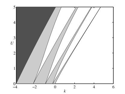
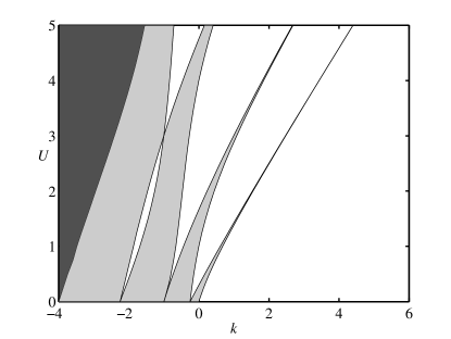
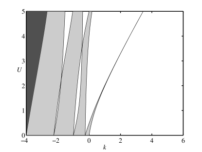
Figure 1: The bandgap structure, as a function of modulation depth $U$ [see Eq. (2)], found from the linearization of Eq. (3) for (a) $D=3\pi/2$, (b) $D=\pi$, and (c) $D=\pi/2$, the respective “duty-cycle” values being $\mathrm{DC}=0.75,~{}0.50,~{}0.25$. Here and in other figures that display ranges of $k$, shaded areas are occupied by Bloch bands. The spectrum was not computed in the black area.

In the SDF model, soliton families were looked for in the first two finite bandgaps of the spectrum. For very small values of the “duty cycle”, namely, $\mathrm{DC}\lesssim 0.05$ and sufficiently large values of $U$, the results are very similar to those reported for the “Dirac-comb” model in Refs. Sukhorukov ; Sukhorukov2 , while they are quite different for the above-mentioned values, $\mathrm{DC}=0.75,~{}0,50,~{}0.25$ and $U=3$, for which systematic results are reported below. Naturally, for fixed $U$ and very small values of $\mathrm{DC}$, solitons cannot exist with the SDF sign of the nonlinearity. In particular, fixing $U=3$, we have found that the solitons disappear at $\mathrm{DC}\leq\left(\mathrm{DC}\right)_{\mathrm{cr}}\approx 0.04$. On the other hand, in the SF model the solitons do not disappear in the same limit, as very narrow solitons with a large total power can be held in a very narrow channel.

III The self-defocusing (SDF) nonlinearity

III.1 Fundamental and higher-order spatially symmetric gap solitons

Different families of GSs are identified by the number of peaks in them. In addition to the fundamental (single-peak) solitons, we have found families of spatially symmetric (even) localized modes with two, three, and four peaks. Figure 2 represents these families by means of respective dependences $Q(k)$, at the three above-mentioned characteristic values of $\mathrm{DC}$, in the first two finite bandgaps. In the case of $\mathrm{DC}=0.25$, the second bandgap is empty, as no soliton solutions could be found in it. It is also necessary to mention that, in the latter case, the higher-order solitons are classified as $2$-, $3$-, and $4$-peak ones by analogy with the situation observed for $\mathrm{DC}=0.75$ and $0.50$, while their actual shape is different, see Fig. 9 below (in fact, numbers $2$, $3$ and $4$ for these solitons pertain not to the number of peaks but rather to the number of channels occupied by each localized mode).

For $\mathrm{DC}=0.75$, the GS families are entirely stable, while, in the intermediate case, $\mathrm{DC}=0.50$, the analysis identifies an intrinsic stability border in the middle of the second bandgap. The transition from stable to unstable solutions occurs at points where the GSs feature a specific flat-top shape, see below.

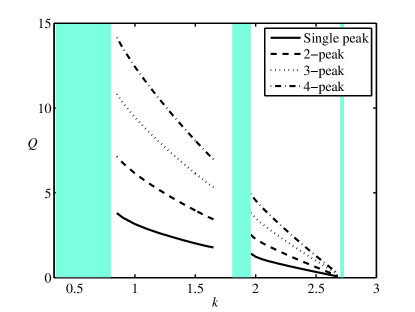
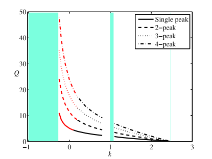
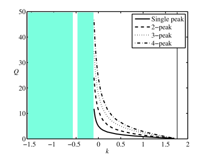
Figure 2: Total power $Q$ versus propagation constant $k$ for fundamental and higher-order gap-soliton families in the defocusing model, is shown at three values of the structural “duty cycle”: $\mathrm{DC}\equiv D/L=0.75$, $0.5$, and $0.25$, in panels (a), (b), and (c), respectively. Families of stable and unstable solutions are shown, severally, by black and red (gray, in the black-and-white version) curves.

For $\mathrm{DC}=0.75$, typical examples of stable fundamental GSs, together with $2$-, $3$- and $4$-peak solitons, are displayed in Fig. 3 and 4, in the first and second bandgaps, respectively. For both $\mathrm{DC}=0.75$ and $\mathrm{DC}=0.50$, maxima and minima of the local power in stable solitons are always observed, respectively, in waveguiding channels and in empty layers between them, while for $\mathrm{DC}=0.25$ the situation is different, see below. Another relevant conclusion is that the $N$-peak solitons may be clearly considered as bound states of $N$ fundamental ones, as suggested by the fact that, as obvious in Fig. 2, the respective powers are related by $Q_{N}\approx NQ_{\mathrm{fund}}$.

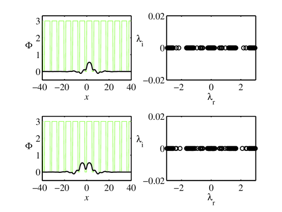
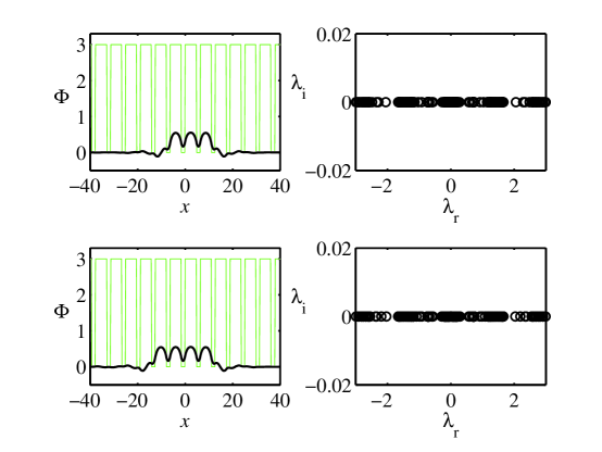
Figure 3: Examples of stable fundamental and double-peak solitons (a), and their three- and four-peak counterparts (b), found in the first bandgap of the defocusing model with $\mathrm{DC}=0.75$, for a fixed value of the propagation constant, $k=2$. In each panel (here and in similar figures below), the right plot shows the spectral plane of stability eigenvalues for the respective soliton, $\lambda\equiv\lambda_{\mathrm{r}}+i\lambda_{\mathrm{i}}$ (the stability in implied by $\lambda_{\mathrm{i}}=0$). Here and in other figures, the background pattern represents the underlying structure of the layered medium.

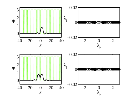
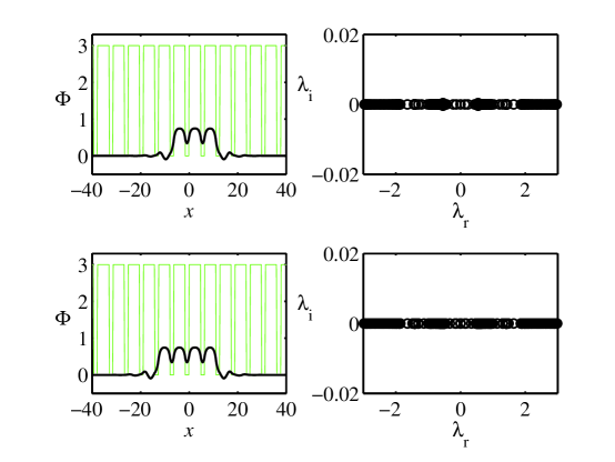
Figure 4: The same as in Fig. 4, but in the second bandgap, for $k=1.3$.

In fact, dependences $Q(k)$ and shapes of the solitons in the SDF model with $\mathrm{DC}=0.75$ are very similar to those known for ordinary GSs in the standard model with the KP potential and uniform repulsive nonlinearity, cf. Refs. Smerzi ; Carr ; Gisin . For $\mathrm{DC}=0.5$, the fundamental and multi-peak GSs in the first bandgap are close to their counterparts displayed in Fig. 3 for $\mathrm{DC}=0.75$. However, as shown in Fig. 5, they are essentially different in the second bandgap of the model with $\mathrm{DC}=0.5$ (hence, different from the ordinary GSs too), showing a trend to flattening.

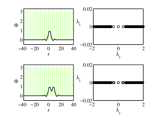
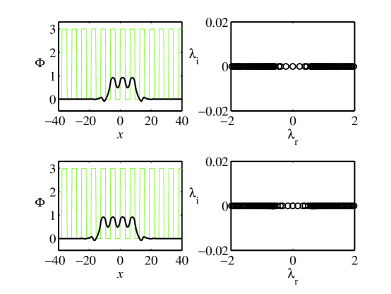
Figure 5: Examples of stable solitons in the second bandgap of the defocusing model with $\mathrm{DC}=0.5$, for a fixed propagation constant, $k=0.4$: (a) a fundamental soliton, with $Q=3.20$, and a double-peak one, with $Q=6.69$; (b) a three- and four-peak solitons, with $Q=10.17$ and $Q=13.65$, respectively.

As said above, a new feature found in the second bandgap of the SDF model with $\mathrm{DC}=0.5$ is destabilization of all branches of the GSs (fundamental and multi-peak ones alike). As seen in Fig. 2(b), this happens at small positive values of $k$. Exactly at the stability border (and close to it, on both sides) all the solitons feature a flat-top shape, as shown in Fig. 6.

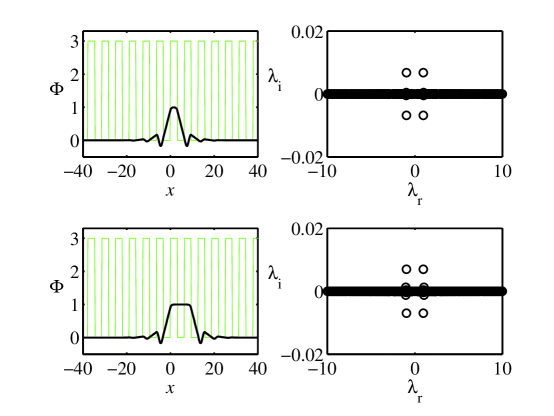
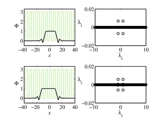
Figure 6: Weakly unstable nearly flat-top solitons found at $k=0$ in the second bandgap of the defocusing model with $\mathrm{CD}=0.50$: (a) A fundamental soliton, with $Q=5.08$, and flat-top counterpart of the double-peak soliton, with $Q=11.33$. (b) Flat-top counterparts of three- and four-peak solitons, with $Q=17.58$ and $23.83$, respectively.

Deeper into the instability region, the higher-order GSs develop inverted shapes, with respect to their stable counterparts, see Fig. 7: on top of the flat-top background, peaks emerge in empty spaces between the waveguiding channels. In this case, the fundamental soliton tends to keep a nearly flat-top shape (although its instability is not essentially weaker than that of its higher-order counterparts), featuring a shallow depression in the central guiding channel. Thus, each localized mode that had $N$ peaks, and $N-1$ troughs between them, in the stable configuration, develops $N-1$ inverted peaks, in locations of the former troughs, after passing the destabilization threshold (which corresponds to the flat-top configuration). In fact, this shape transformation suggests that, with the increase of total power $Q$, the effective repulsive nonlinear potential becomes stronger than the trapping linear one, pushing the wave into the empty space and destabilizing the trapped state.

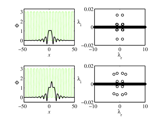
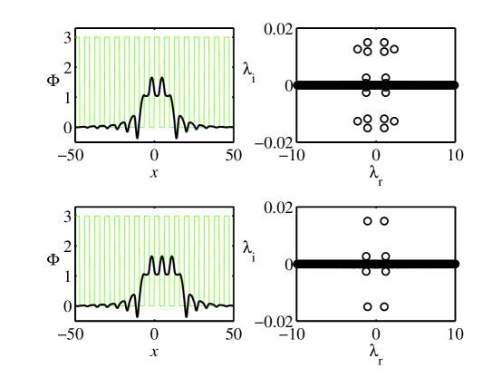
Figure 7: Unstable solitons with the inverted shape (i.e., with local power maxima in empty layers). All the examples are shown for $k=-0.22$. The top and bottom plots in panel (a) display, respectively, a fundamental soliton, with $Q=9.17$ , and the former double-peak soliton (which actually features a single-peak structure, as a result of the inversion), with $Q=21.06$. The top and bottom plots in panel (b) display, respectively, inverted counterparts of former three- and four-peak solitons, with powers $Q=30.88$ and $Q=42.74$.

When the flat-top fundamental GS becomes unstable, direct simulations demonstrate that growing perturbations slowly destroy it, see Fig. 8(a). As for unstable flat-top counterparts of stable multi-peak solitons, the perturbation first splits them back into a multi-peak structure, and then gradually destroys them. A typical example of this scenario of the instability development is shown, for the GS of the $3$-peak type, in Fig. 8(b).

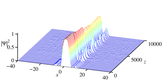
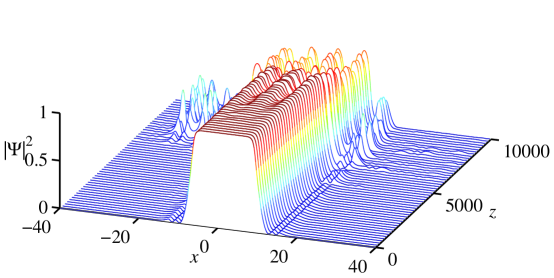
Figure 8: (a) The evolution of an unstable fundamental soliton with $k=-0.15$ and $Q=17.58$ in the self-defocusing model with $\mathrm{DC}=0.5$. (b) The same for an unstable flat-top soliton belonging to the three-peak family, with $k=0$ and $Q=17.58$.

At small values of $\mathrm{DC}$, such as $\mathrm{DC}=0.25$, GSs of all types are found only in the first bandgap. A peculiarity of the soliton families in this case is that they feature peaks in empty layers, being, nevertheless, completely stable, on the contrary to their unstable counterparts in the second bandgap found at $\mathrm{DC}=0.50$, which demonstrate a similar structure, as described above. Examples of these stable solitons are displayed in Fig. 9.

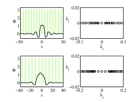
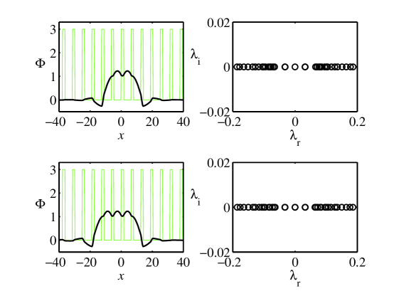
Figure 9: Examples of stable gap solitons in the first bandgap of the self-defocusing model with $\mathrm{DC}=0.25$. In panel (a), the top and bottom plots represent, respectively, a fundamental soliton (i.e., the one localized in a single channel), with $k=-0.1$ and $Q=11.77$, and a soliton occupying two channels, with $k=-0.05$ and $Q=15.26$. Panel (b) displays higher-order solitons occupying three and four channels, with $Q=23.18$ and $31.60$, respectively, both pertaining to $k=-0.05$. Note that these stable solitons feature local maxima of the power in empty channels.

III.2 Antisymmetric gap solitons

In addition to the two-peak states displayed above, which may be considered as symmetric bound states of fundamental GSs, a family of their antisymmetric (“twisted”) bound states can be readily found too. These bound states turn out to be stable in the first finite bandgap, but unstable in the second, both for $\mathrm{DC}=0.75$ and $0.50$. In the case of $\mathrm{DC}=0.25$, the second bandgap stays empty, as shown above, therefore bound states do not exist in that bandgap either, while twisted bound states of fundamental GSs exist and are stable in the first bandgap. These findings are presented in Figs. 10 and 11. An example of the evolution (gradual destruction) of an unstable antisymmetric bound state in the second bandgap is shown (for $\mathrm{DC}=0.50$) in Fig. 12(a).

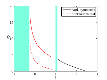
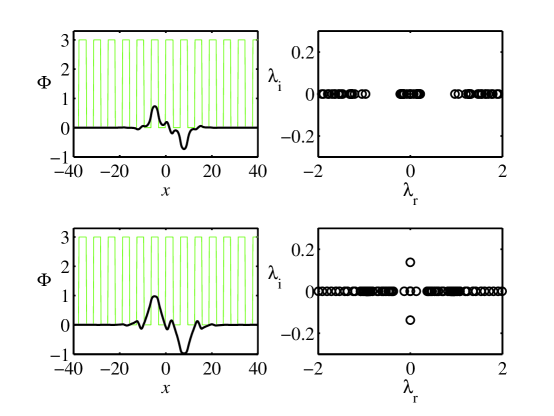
Figure 10: (a) The total power of antisymmetric (“twisted”) bound states of fundamental gap solitons versus the propagation constant, in the defocusing model with $\mathrm{DC}=0.50$. The same characteristic is also shown for the family of subfundamental solitons in the second bandgap. Typical examples of stable ($k=1.2$ and $Q=3.19$) and unstable ($k=0.1$ and $Q=8.17$) antisymmetric bound states, in the first and second bandgaps, are shown in panel (b).

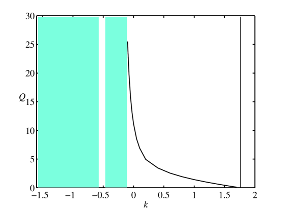
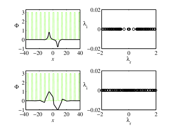
Figure 11: (a) The total power of the antisymmetric bound state versus the propagation constant, in the first bandgap of the defocusing model with $\mathrm{DC}=0.25$. (b) Examples of these stable antisymmetric bound states: (top panel) $k=0.5$ and $Q=2.96$; (bottom panel) $k=0$ and $Q=11.14$.

It is known that the combination of a periodic potential and spatially uniform SDF nonlinear term (whose power may be different from cubic SKA ) gives rise to an additional family of weakly unstable subfundamental solitons, in the second bandgap only. The solitons were given this name because their total power is smaller than that of the fundamental solitons found in the same bandgap we . Each subfundamental soliton is an antisymmetric one, but it is not a bound state of fundamental GSs, as it is localized as tightly as fundamental solitons (i.e., it is a twisted state squeezed, essentially, into a single guiding channel). Subfundamental solitons can also be found in the second bandgap of the present model, for $\mathrm{DC}=0.75$ and $\mathrm{DC}=0.50$ (they do not exist at $\mathrm{DC}=0.25$, as in that case the second bandgap is empty, as shown above). For $\mathrm{DC}=0.50$, dependence $Q(k)$ for the family of subfundamental solitons is shown by the dashed curve in Fig. 10(a), and an example of the subfundamental soliton is displayed in Fig. 12(b). Similar to the ordinary model, the subfundamental solitons in the present model are weakly unstable, and spontaneously transform themselves into fundamental GSs belonging to the first bandgap.

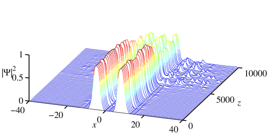
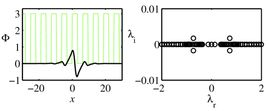
Figure 12: (a) The evolution of an unstable “twisted” soliton (antisymmetric bound state of two fundamental gap solitons) in the second bandgap, for $k=0.1$ and $Q=8.17$, in the self-defocusing model with $\mathrm{DC}=0.5$. (b) An example of a weakly unstable subfundamental soliton (for $k=0.1$ and $Q=2.43$) found in the second bandgap of the model with $\mathrm{DC}=0.50$.

IV The self-focusing (SF) nonlinearity

In model with SF the sign of the nonlinear term, solitons can be readily found in the semi-infinite gap. As might be expected, they are quite similar to solitons previously found in the model with the KP periodic potential and uniform nonlinearity Smerzi . In Fig. 13, we display a set of respective curves $Q\left(k\right)$ for different values of $\mathrm{DC}$, and a typical example of a stable soliton, for $\mathrm{DC}=0.25$. The stability of the entire soliton family complies with the prediction of the VK criterion VK , according to which the positive slope of the curve, $dQ/dk>0$, is a necessary stability condition (this criterion is irrelevant to SDF models). As concerns the example of the soliton displayed in Fig. 13, it is worthy to note that the soliton remains trapped almost entirely within a single waveguiding channel, even when it is narrow (corresponding to $\mathrm{DC}=0.25$). The same feature has been observed in all other cases.

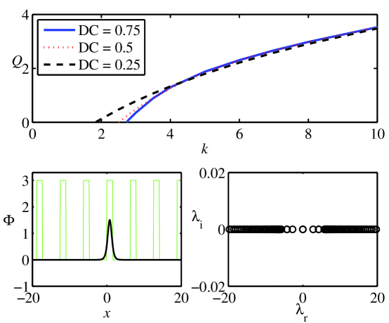
Figure 13: The top plot shows the total power versus the propagation constant for families of solitons found in the semi-infinite gap of the self-focusing model. The bottom plot displays a typical example of a stable soliton, with $k=6$ and $Q=2.21$, trapped in a narrow channel corresponding to $\mathrm{DC}=0.25$.

In the parameter region investigated in the framework of this work, we have not found multi-peak solitons in the semi-infinite gap. Solitons in finite bandgaps of the SF model were not found either (unlike the models combining a periodic potential and spatially uniform cubic-quintic nonlinearity, which realizes the competition between SF and SDF terms Gisin ; China ).

V Conclusion

The objective of this work was to develop a systematic analysis of spatial solitons in the model of 1D photonic crystals, built as the periodic alternation of nonlinear waveguiding channels, of width $D$, and empty layers between them, of width $L-D$. The main parameter of the model is the structural “duty cycle”, $\mathrm{DC~{}}\equiv D/L$. We have concentrated, chiefly, on the model with the SDF (self-defocusing) sign of the nonlinearity in the channels, as this setting makes it possible to study new effects due the competition between the linear trapping potential and its effective repulsive nonlinear counterpart. Various types of solitons in this model have been found in the first two finite bandgaps (alias Bragg-reflection gaps) of the SDF model. The family of fundamental solitons has been constructed too in the semi-infinite gap (alias the one accounted for by the total internal reflection) of the system with the SF (self-focusing) nonlinearity. In the SDF model with $\mathrm{DC}=0.75$, and also in the SF one, the solitons are quite similar to their counterparts in the respective models with the uniform nonlinearity. On the other hand, the solitons residing in the second bandgap of the SDF model with $\mathrm{DC}=0.50$ strongly differ from the ordinary GSs: both fundamental solitons and their spatially symmetric bound states pass a destabilization point, with the increase of the total power. At this point, the solitons feature a flat-top shape, while beyond it the shape is inverted, with local maxima emerging in empty layers. The shape inversion and destabilization of the solitons are explained by the competition between the linear trapping potential and its nonlinear repulsive counterpart. In the system with narrow guiding channels, $\mathrm{DC}=0.25$, GSs are found only in the first finite bandgap, where they are stable (both fundamental ones and their bound states), despite the fact that they feature the inverted shape.

New properties of the fundamental solitons and their bound complexes in the system with moderate or low values of $\mathrm{DC}$, $0.50$ and $0.25$, may find applications to the design of all-optical data-processing schemes based on spatial solitons in planar settings.
ACKNOWLEDGMENTS
The work of T. Mayteevarunyoo is supported, in a part, by a postdoctoral fellowship from the Pikovsky-Valazzi Foundation, by the Israel Science Foundation through the Center-of-Excellence grant No. 8006/03, and by the Thailand Research Fund under grant No. MRG5080171.

References

- (1) E. Yablonovitch, “Photonic band-gap structures”, J. Opt. Soc. Am. B 10, 283-295 (1993).
- (2) E. Yablonovitch, “Photonic crystals”, J. Mod. Opt. 41, 173-194 (1994).
- (3) T. F. Krauss and R. M. De la Rue, “Photonic crystals in the optical regime – past, present and future”, Progr. Quant. Electr. 23, 51-96 (1999).
- (4) M. Soljacic and J. D. Joannopoulos, “Enhancement of nonlinear effects using photonic crystals”, Nature Materials 3, 211-219 (2004).
- (5) B. Maes, P. Bienstman, and R. Baets, “Bloch modes and self-localized waveguides in nonlinear photonic crystals”, J. Opt. Soc. Am. B 22, 613-619 (2005).
- (6) P. S. J. Russell, “Photonic-crystal fibers”, J. Lightwave Tech. 24, 4729-4749 (2006).
- (7) E. Istrate and E. H. Sargent, “Photonic crystal heterostructures and interfaces”, Rev. Mod. Phys. 78, 455-481 (2006).
- (8) K. Busch, G. von Freymann, S. Linden, S. F. Mingaleev, L. Tkeshelashvili, and M. Wegener, “Periodic nanostructures for photonics”, Phys. Rep. 444, 101-202 (2007).
- (9) N. Akozbek and S. John, “Optical solitary waves in two- and three-dimensional nonlinear photonic band-gap structures”, Phys. Rev. E 57, 2287-2319 (1998).
- (10) C. Conti, S. Trillo, and G. Assanto, “Energy localization in photonic crystals of a purely nonlinear origin”, Phys. Rev. Lett. 85, 2502-2505 (2000).
- (11) S. F. Mingaleev, Y. S. Kivshar, and R. A. Sammut, “Long-range interaction and nonlinear localized modes in photonic crystal waveguides”, Phys. Rev. E 62, 5777-5782 (2000).
- (12) S. F. Mingaleev and Y. S. Kivshar, “Self-trapping and stable localized modes in nonlinear photonic crystals”, Phys. Rev. Lett. 86, 5474-5477 (2001).
- (13) A. A. Sukhorukov and Y. S. Kivshar, “Spatial optical solitons in nonlinear photonic crystals”, Phys. Rev. E 65, 036609 (2002).
- (14) A. A. Sukhorukov and Y. S. Kivshar, “Nonlinear guided waves and spatial solitons in a periodic layered medium”, J. Opt. Soc. Am. B 19, 772-781 (2002).
- (15) P. Xie, Z. Q. Zhang, and X. D. Zhang, “Gap solitons and soliton trains in finite-sized two-dimensional periodic and quasiperiodic photonic crystals”, Phys. Rev. E 67, 026607 (2003).
- (16) A. Ferrando, M. Zacarés, P. Fernández de Córdoba, D. Binosi, and J. A. Monsoriu, “Spatial soliton formation in photonic crystal fibers”, Opt. Exp. 11, 452-459 (2003).
- (17) A. Ferrando, M. Zacarés, P. Fernández de Córdoba, D. Binosi, and J. A. Monsoriu, “Vortex solitons in photonic crystal fibers”, Opt. Exp. 12, 817-822 (2004).
- (18) Y. V. Kartashov, V. A. Vysloukh, and L. Torner, “Soliton trains in photonic lattices”, Opt. Exp. 12, 2831-2837 (2004).
- (19) B. Maes, P. Bienstman, and R. Baets, “Switching in coupled nonlinear photonic-crystal resonators”, J. Opt. Soc. Am. B 22, 1778-1784 (2005).
- (20) N. K. Efremidis, S. Sears, D. N. Christodoulides, J. W. Fleischer, and M. Segev, “Discrete solitons in photorefractive optically induced photonic lattices”, Phys. Rev. E 66, 046602 (2002).
- (21) J. W. Fleischer, M. Segev, N. K. Efremidis, and D. N. Christodoulides, “Observation of two-dimensional discrete solitons in optically induced nonlinear photonic lattices”, Nature 422, 147-150 (2003).
- (22) D. Neshev, E. Ostrovskaya, Y. Kivshar, and W. Królikowski, “Spatial solitons in optically induced gratings”, Opt. Lett. 28, 710-712 (2003).
- (23) G. Bartal, O. Manela, O. Cohen, J. W. Fleischer, and M. Segev, “Observation of second-band vortex solitons in 2D photonic lattices”, Phys. Rev. Lett. 95, 053904 (2005).
- (24) N. A. R. Bhat and J. E. Sipe, “Optical pulse propagation in nonlinear photonic crystals”, Phys. Rev. E 64, 056604 (2001).
- (25) D. N. Christodoulides and N. K. Efremidis, “Discrete temporal solitons along a chain of nonlinear coupled microcavities embedded in photonic crystals”, Opt. Lett. 27, 568-570 (2002).
- (26) J. K. S. Poon, J. Scheuer, S. Mookherjea, G. T. Paloczi, Y. Y. Huang, and A. Yariv, “Matrix analysis of microring coupled-resonator optical waveguides”, Opt. Exp. 12, 90-103 (2004).
- (27) B. I. Mantsyzov, I. V. Mel’nikov, and J. Stewart Aitchison, “Controlling light by light in a one-dimensional resonant photonic crystal”, Phys. Rev. E 69, 055602(R) (2004).
- (28) A. V. Husakou and J. Herrmann, “Supercontinuum generation of higher-order solitons by fission in photonic crystal fibers”, Phys. Rev. Lett. 87, 203901 (2001).
- (29) J. Herrmann, U. Griebner, N. Zhavoronkov, A. Husakou, D. Nickel, J. C. Knight, W. J. Wadsworth, P. S. J. Russell, and G. Korn, “Experimental evidence for supercontinuum generation by fission of higher-order solitons in photonic fibers”, Phys. Rev. Lett. 88, 173901 (2002).
- (30) F. Luan, J. C. Knight, P. St. J. Russell, S. Campbell, D. Xiao, D. T. Reid, B. J. Mangan, D. P. Williams, and P. J. Roberts, “Femtosecond soliton pulse delivery at 800nm wavelength in hollow-core photonic bandgap fibers”, Opt. Exp. 12, 835-840 (2004).
- (31) A. Efimov, A. V. Yulin, D. V. Skryabin, J. C. Knight, N. Joly, F. G. Omenetto, A. J. Taylor, and P. Russell, “Interaction of an optical soliton with a dispersive wave”, Phys. Rev. Lett. 95, 213902 (2005).
- (32) J. F. Corney and O. Bang, “Solitons in quadratic nonlinear photonic crystals”, Phys. Rev. E Volume: 64, 047601 (2001).
- (33) C. Kittel, Introduction to Solid State Physics (Wiley: New York, 1995).
- (34) W. Li and A. Smerzi, Phys. Rev. E 70, 016605 (2004).
- (35) B. T. Seaman, L. D. Carr, and M. J. Holland, “Nonlinear band structure in Bose-Einstein condensates: Nonlinear Schrödinger equation with a Kronig-Penney potential”, Phys. Rev. A 71, 033622 (2005).
- (36) I. M. Merhasin, B. V. Gisin, R. Driben, and B. A. Malomed, “Finite-band solitons in the Kronig-Penney model with the cubic-quintic nonlinearity”, Phys. Rev. E 71, 016613 (2005).
- (37) J. Wang, F. Ye, L. Dong, T. Cai, and Y.-P. Li, “Lattice solitons supported by competing cubic–quintic nonlinearity”, Phys. Lett. A 339, 74 (2005).
- (38) G. L. Alfimov, V. V. Konotop, and M. Salerno, Europhys. Lett., “Matter solitons in Bose-Einstein condensates with optical lattices”, Europhys. Lett. 58, 7-13 (2002).
- (39) B. B. Baizakov, V. V. Konotop, and M. Salerno, “Regular spatial structures in arrays of Bose–Einstein condensates induced by modulational instability”, J. Phys. B: At. Mol. Opt. Phys. 35, 5105–5119 (2002).
- (40) P. J. Y. Louis, E. A. Ostrovskaya, C. M. Savage, and Y. S. Kivshar, “Bose-Einstein condensates in optical lattices: Band-gap structure and solitons”, Phys. Rev. A 67, 013602 (2003).
- (41) H. Sakaguchi and B. A. Malomed, “Matter-wave solitons in nonlinear optical lattices”, Phys. Rev. E 72, 046610 (2005).
- (42) Y. Sivan, G. Fibich, and M. I. Weinstein, “Waves in nonlinear lattices: Ultrashort optical pulses and Bose-Einstein condensates”, Phys. Rev. Lett. 97, 193902 (2006).
- (43) F. Abdullaev, A. Abdumalikov, and R. Galimzyanov, “Gap solitons in Bose–Einstein condensates in linear and nonlinear optical lattices”, Phys. Lett. A 367, 149-155 (2007).
- (44) Z. Rapti, P. G. Kevrekidis, V. V. Konotop and C. K. R. T. Jones, “Solitary waves under the competition of linear and nonlinear periodic potentials”, J. Phys. A: Math. Theor. 40, 14151-14163 (2007).
- (45) T. Mayteevarunyoo and B. A. Malomed, “Stability limits for gap solitons in a Bose-Einstein condensate trapped in a time-modulated optical lattice”, Phys. Rev. A 74, 033616 (2006).
- (46) B. A. Malomed, Z. H. Wang, P. L. Chu, and G. D. Peng, “Multichannel switchable system for spatial solitons”, J. Opt. Soc. Am. B 16, 1197-1203 (1999).
- (47) N. G. Vakhitov and A. A. Kolokolov, “Stationary solutions of the wave equation in a medium with nonlinearity saturation”, Izv. Vyssh. Uchebn. Zaved., Radiofiz. 16, 10120 (1973) [in Russian; English translation: Radiophys. Quantum. Electron. 16, 783 (1973)]; see also L. Bergé, “Wave collapse in physics: principles and applications to light and plasma waves”, Phys. Rep. 303, 259-370 (1998).
- (48) B. Deconinck, F. Kiyak, J. D. Carter, and J. N. Kutz, “SpectrUW: A laboratory for the numerical exploration of spectra of linear operators, “Math. Comput. Simul. 74, 370-378 (2007).
- (49) S. Adhikari and B. A. Malomed, “Tightly bound gap solitons in a Fermi gas”, Europhys. Lett. 79, 50003 (2007).