Full-Potential Multiple Scattering Theory with Space-Filling Cells for bound and continuum states

Abstract

We present a rigorous derivation of a real space Full-Potential Multiple-Scattering-Theory (FP-MST) that is free from the drawbacks that up to now have impaired its development (in particular the need to expand cell shape functions in spherical harmonics and rectangular matrices), valid both for continuum and bound states, under conditions for space-partitioning that are not excessively restrictive and easily implemented. In this connection we give a new scheme to generate local basis functions for the truncated potential cells that is simple, fast, efficient, valid for any shape of the cell and reduces to the minimum the number of spherical harmonics in the expansion of the scattering wave function. The method also avoids the need for saturating ’internal sums’ due to the re-expansion of the spherical Hankel functions around another point in space (usually another cell center). Thus this approach, provides a straightforward extension of MST in the Muffin-Tin (MT) approximation, with only one truncation parameter given by the classical relation $l_{\rm max}=kR_{b}$, where $k$ is the electron wave vector (either in the excited or ground state of the system under consideration) and $R_{b}$ the radius of the bounding sphere of the scattering cell. Moreover, the scattering path operator of the theory can be found in terms of an absolutely convergent procedure in the $l_{\rm max}\rightarrow\infty$ limit. Consequently, this feature provides a firm ground to the use of FP-MST as a viable method for electronic structure calculations and makes possible the computation of x-ray spectroscopies, notably photo-electron diffraction, absorption and anomalous scattering among others, with the ease and versatility of the corresponding MT theory. Some numerical applications of the theory are presented, both for continuum and bound states.

1 Introduction

At its most basic, Multiple scattering Theory (MST) is a technique for solving a linear partial differential equation over a region of space with certain boundary conditions. It is implemented by dividing the space into non-overlapping domains (cells), solving the differential equation separately in each of the cells and then assembling together the partial solutions into a global solution that is continuous and smooth across the whole region and satisfies the given boundary conditions.

As such MST has been applied to the solution of many problems drawn both from classic as well as quantum physics, ranging from the study of membranes and electromagnetism to the quantum-mechanical wave equation. In quantum mechanics it has been widely used to solve the Schrödinger equation (SE) ( or the associated Lippmann-Schwinger equation (LSE)) both for scattering and bound states. It was proposed originally by Korringa and by Kohn and Rostoker (KKR) as a convenient method for calculating the electronic structure of solids  [1, 2] and was later extended to polyatomic molecules by Slater and Johnson  [3]. A characteristic feature of the method is the complete separation between the potential aspect of the material under study, embodied in the cell scattering power, from the structural aspect of the problem, reflecting the geometrical position of the atoms in space.

Applications of the KKR method were first made within the so-called muffin-tin (MT) approximation for the potential. In this approximation the potential is confined within non-overlapping spheres, where it is spherically symmetrized, and takes a constant value in the interstitial region. Moreover, although spherical symmetry is not formally necessary, the condition that the bounding spheres do not overlap was thought to be necessary for the validity of the theory. Despite this approximation the method is complicated and demanding from a numerical point of view and as a band-structure method it was therefore superseded by more efficient linearized methods, such as the linearized muffin-tin-orbital method (LMTO)  [4] and the linearized augmented-plane-wave method (LAPW).  [5]

Full-potential versions of these band methods have also been introduced in recent years. However, none of these methods can match the power and versatility of a full-potential method based on the formalism of MST, either in terms of providing a complete solution of the SE or in the range of problems that could be treated. In particular, none of these methods leads easily to the construction of the Green’s Function (GF) which is indispensable in the study of a number of properties of many physical systems.

Due to these reasons, in the last two decades, the KKR method has experienced a revival in the framework of the Green’s function method (KKR-GF). Indeed, due to the introduction of the complex energy integration, it was found that the method is well suited for ground-state calculations, with an efficiency comparable to typical diagonalization methods. An host of problems became in this way tractable, ranging from solids with reduced symmetry (like e.g. isolated impurities in ordered crystal, surfaces, interfaces, layered systems, etc..) to randomly disordered alloys in the coherent potential approximation (CPA).

At the same time it soon became clear that the MT approximation was not adequate to the treatment of systems with reduced symmetry or for the calculation of lattice forces and relaxation. In order to deal with these problems a number of groups developed a full potential (FP) KKR-GF method, obtaining very good results, comparable with full-potential LAPW method (FLAPW), for what concerns total energy calculations, lattice forces, relaxation around an impurity, ( [6, 7, 8, 9, 10] and Refs. therein). Due to their method of generating the single site solutions and the cell t-matrix, the additional numerical effort required for the implementation of the FP-MS scheme scales only linearly with the number of non-equivalent atoms and is not significantly greater than in the MT case.

In this development the authors took an empirical attitude toward some fundamental problems related to the extension of MST to the full-potential case, like the strongly debated question of the l-convergence of the theory or the need to converge “internal” sums arising from the re-expansion of the free Green’s function around two sites, which entails the unwanted feature of the introduction of rectangular matrices into the theory. [11] Without getting involved into ab initio questions, they just use square matrices for the structural Green’s Function $G^{nn^{\prime}}_{LL^{\prime}}(E)$ needed to calculate the Green’s Function of the system (see e.g. Eqs. (6) and (9) in Ref. [9]) and truncate the l-expansion to $l_{\rm max}=$ 3 or 4, obtaining in this way the same accuracy as the FLAPW method.

Some observations are in order at this point. First, the FP method in the framework of MST has been initially developed only for periodic systems in two or three dimensions and for states below the Fermi level. To our knowledge, its extension to treat bound and continuum states of polyatomic molecules and in general real space applications of the method have progressed very slowly and have been scarce. Secondly, the generation of the local solutions of the SE with truncated cells in the FP extension of the MST has up to now involved the expansion of the cell shape function in spherical harmonics, which might create convergence problems, as discussed below. Thirdly, the FP extension of MST has generated a lot of controversies that have gone on for more than thirty years  [12]. Some of the problems have found a solution and we refer the reader to the book of Gonis and Butler  [13] for a comprehensive review of the state of the art in this field (in particular see their chapter 6). However, questions like the l-convergence of the theory or the use of square matrices are still matter of debate and some rigorous answer should be given to them.

As mentioned above, applications to states well above the Fermi energy, as required in the simulations of x-ray spectroscopies, like absorption, photo-emission, anomalous scattering, etc…, have been scarce. In the words of Ref.  [13], “the feeling that one should calculate the “near-field-corrections” (NFC), coupled with the need to solve a fairly complicated system of coupled differential equation to determine the local (cell) solutions (based on the phase function method) has contributed greatly to the slow development of a FP method based on MST”. It was only after it was realized that NFC are not necessary and a new method to generate local solutions was found that progress became faster, at least in the calculation of the electronic structure of solids. ( [6, 7, 8, 9, 10] and Refs. therein) The only remaining drawback was and is the truncation of the potential at the cell boundary which is still performed via a shape function expanded in spherical harmonics. Added to this there is the feeling that one should still converge the “internal” sums leading to the use of rectangular matrices in the angular momentum (AM) indexes, although this last step is sometimes ignored without justifications. Last, but not least, the question of the l-convergence of the theory remains unsettled.

For all these reasons FP codes based on MST for the calculation of x-ray spectroscopies are not very numerous. We mention here the work by Huhne and Ebert  [14] on the calculation of x-ray absorption spectra using the FP spin-polarized relativistic MST and that of Ankudinov and Rehr  [15] in the scalar relativistic approximation. These authors use the potential shape function to generate the local basis functions which are at the heart of MST. The expansion of the shape function and the cell potential in spherical harmonics leads to a high number of spherical components in the coupled radial equations that becomes progressively cumbersome to handle and time consuming with increasing energy and in absence of symmetry. This feature might also be at the origin of another problem related with the saturation of ”internal” sums in the MSE  [13], as discussed later in this paper. Moreover no critical discussion is devoted in their work to the l-convergence problems of MST or the use of square matrices in the theory.

Another code based on a version of the MST that uses non overlapping spherical cells and treats the interstitial potential in the Born approximation is that of Foulis et al.  [16, 17] This method however treats in an approximate way the potential in the interstitial region and moreover looses one of the major advantages of the MST, namely the separation between dynamics and geometry in the solution of the scattering problem. Foulis  [18] is now developing an exact FP-MS scheme based on distorted waves in the interstitial region that seem to be promising, but its numerical implementation is still to come.

There are other codes that simulates x-ray spectroscopies and are not based on MST: that of Joly  [19] is based on the discretization of the Laplacian in three dimensions (finite-difference method (FDM)), where the SE is solved in a discretized form on a three-dimensional grid, the values of the scattering wave-function being the unknowns. This method is however limited to cluster sizes of the order of 20 atoms (without symmetry), due to the high memory requirement when the number of mesh points increases with the dimensions of the cluster. Finally a method based on the pseudo-potential theory to calculate x-ray absorption is worth mentioning. [20] It can easily cope with clusters of many atoms (300 and more) with a computational effort that scales linearly with the number of atoms. One of its drawback is its little physical transparency and the fact that it has been applied only to calculate x-ray absorption spectra. Also, relaxation around the core hole must be taken into account by super-cell calculations and there is little flexibility to deal with energy-dependent complex potentials.

The purpose of the present paper is the rigorous derivation of a real space FP-MST, valid both for continuum and bound states, that is free from the drawbacks hinted to above, in particular the need to use cell shape functions and rectangular matrices, under conditions for space-partitioning that are not excessively restrictive and easily implemented (see beginning of Section 3). In connection with this we shall present a new scheme to generate local basis functions for the truncated potential cells that is simple, fast, efficient, valid for any shape of the cell and reduces to the minimum the number of spherical harmonics in the expansion of the scattering wave function. Finally we shall also address the problem of the l-convergence of the theory, giving a positive answer to this debated question.

Even though this work is primarily motivated by applications in spectroscopy, it will be clear from the context that bound states can be treated as well. Actually the method can also work for complex energy values, so that one can take advantage of the fact that the solution of the Schrödinger equation is analytical in the energy plane, as is the associated Green’s function, except for cuts and poles on the real axis. Therefore spectroscopy is only one regime of applications.

Section 2 of this paper presents the new scheme to generate local basis functions and tests it against known solutions for potentials cells with and without shape truncation. Section 3 provides a new derivation of the FP-MST that allows us to work with square matrices for the phase functions $S_{LL^{\prime}}$ and $E_{LL^{\prime}}$ and for the cell $T_{LL^{\prime}}$ matrix with only one truncation parameter, contrary to the present accepted view. [13] Due to their importance in the theory, various equivalent forms for the Green’s function are presented in this scheme. This latter is extended to the calculation of bound states of polyatomic molecules and tested against the known eigenvalues of the hydrogen molecular ion. Section 4 discusses the strongly debated problem of the l-convergence of the theory and provides a truncation procedure that converges absolutely in the $l_{\rm max}\rightarrow\infty$ limit.

Section 5 reports one additional application of the present FP-MS theory besides those already presented in Ref.s  [21] and  [22], namely the calculation of the absorption cross section in the case of linear molecules ($Br_{2}$ diatomic molecule), where the improvement of over the MT approximation is quite dramatic. Moreover, with an eye to using the theory to study the performance of model optical potentials, Section 5 also presents a preliminary application of the non-MT (NMT) approach to the study of the relative performance of the Hedin-Lundqvist (HL) and the Dirac-Hara (DH) potentials in the case of a transition metal. Finally Section 6 presents the conclusions of the present work. A preliminary and partial account of this latter has been presented in Ref.s  [21] and  [22].

2 Local Basis functions for single truncated potential cells

A characteristic feature of MST is that it does not rely on a finite basis set for the expansion of the global wave function inside each cell as all other methods of electronic structure calculations do. Instead it relies on expanding the global solution in terms of local solutions of the Schrödinger equation at the energy of interest, which can be regarded as an optimally small, energy adapted basis set [9]. Therefore it is essential for the practical implementation of the theory to devise an efficient numerical method to generate them. We shall consider Williams and Morgan (WM) basis functions $\Phi_{L}({\bf r})$  [23] which inside each cell are local solutions of the SE and behave at the origin as $J_{L}({\bf r})$ for $r\rightarrow 0$. Throughout the paper we shall use real spherical harmonics and shall put for short $J_{L}({\bf r};k)\equiv j_{l}(kr)Y_{L}(\hat{\bf r})$, $N_{L}({\bf r};k)\equiv n_{l}(kr)Y_{L}(\hat{\bf r})$ and $\tilde{H}_{L}^{+}({\bf r};k)\equiv-ikh_{l}^{+}(kr)Y_{L}(\hat{\bf r})$, where $j_{l},n_{l},h_{l}$ denote respectively spherical Bessel, Neumann and Hankel functions of order $l$. The truncated cell potential $V(r,\hat{\bf r})$ is defined to coincide with the global system potential inside the cell and to be equal to zero (or to a constant) outside. As mentioned in the introduction we want to avoid the expansion of the truncated cell shape function (or equivalently of the truncated potential) in spherical harmonics due to convergence problems. However we observe that, even if the potential has a step, the wave function and its first derivative are continuous, so that its angular momentum expansion is well behaved and even converges uniformly in $\hat{\bf r}$. [24] Therefore we can safely write $\Phi_{L}({\bf r})=\sum_{L^{\prime}}R_{L^{\prime}L}(r)Y_{L^{\prime}}(\hat{\bf r})$ and this expression can be integrated term by term under integral sign.

2.1 Three-dimensional Numerov method

In order to generate the basis functions we write the SE in polar coordinates for the function $P_{L}({\bf r})=r\Phi_{L}({\bf r})$

$$\left[\frac{d^{2}}{dr^{2}}+E-V(r,\hat{\bf r})\right]P_{L}(r,\hat{\bf r})=\frac{1}{r^{2}}\tilde{L}^{2}P_{L}(r,\hat{\bf r})$$ (1)

where $\tilde{L}^{2}$ is the angular momentum operator, whose action on $P_{L}(r,\hat{\bf r})$ can be calculated as:

$$\tilde{L}^{2}P_{L}(r,\hat{\bf r})=\sum_{L^{\prime}}l^{\prime}(l^{\prime}+1)rR_{L^{\prime}L}(r)Y_{L^{\prime}}(\hat{\bf r})$$ (2)

Equation (1) in the variable $r$ looks like a second order equation with an inhomogeneous term. Accordingly we use Numerov’s method to solve it. As is well known, putting $f_{i,j}^{L}=P_{L}(r_{i},\hat{\bf r}_{j})$ and dropping for simplicity the index $L$, the associated three point recursion relation is

$$A_{i+1,j}f_{i+1,j}-B_{i,j}f_{i,j}+A_{i-1,j}f_{i-1,j}=g_{i,j}-\frac{h^{6}}{240}f_{i,j}^{\rm vi}$$ (3)

where,

$$A_{i,j} = 1-\frac{h^{2}}{12}v_{i,j}$$

$$B_{i,j} = 2+\frac{5h^{2}}{6}v_{i,j}=12-10A_{i,j}$$

$$v_{i,j} = V(r_{i},\hat{\bf r}_{j})-E$$

$$g_{i,j} = \frac{h^{2}}{12}[q_{i+1,j}+10q_{i,j}+q_{i-1,j}]$$

$$q_{i,j} = \frac{1}{r_{i}^{2}}\sum_{L^{\prime}}l^{\prime}(l^{\prime}+1)r_{i}R_{L^{\prime}L}(r_{i})Y_{L^{\prime}}(\hat{\bf r}_{j})$$ (4)

Here $i$ is an index of radial mesh and $j$ an index of angular points on a Lebedev surface grid.  [25] Obviously $r_{i}R_{L^{\prime}L}(r_{i})=\sum_{j}w_{j}P_{L}(r_{i},\hat{\bf r}_{j})Y_{L^{\prime}}(\hat{\bf r}_{j})$, where $w_{j}$ is the weight function for angular integration associated with the chosen grid. The number of surface points $N_{Leb}$ is given by $N_{Leb}\approx(2l_{\rm max}+1)^{2}/3$ as a function of the maximum angular momentum used [26], taking into account that one integrates the product of two spherical harmonics. As it is, we cannot use Eq. (3) to find $f_{i+1,j}$ by iteration, from the knowledge of $f_{i,j}$ and $f_{i-1,j}$ at all the angular points, since the ”inhomogeneous” term $q_{i+1,j}$ is not expressible in terms of $f_{i+1,j}$ due to the last line of Eq. (4) and is calculated at the radial mesh point $i+1$.

We first eliminate this point from the expression of $g_{i,j}$, observing that

$$g_{i,j} = \frac{h^{2}}{12}\left[q_{i+1,j}+10q_{i}+q_{i-1,j}\right]$$

$$= \frac{h^{2}}{12}\left[\frac{q_{i+1,j}-2q_{i}+q_{i-1,j}}{h^{2}}h^{2}+12q_{i,j}\right]$$

The second order central difference is given by  [27]

$$q_{i+1}-2q_{i}+q_{i-1} = h^{2}q_{i}^{\prime\prime}+\frac{h^{4}}{12}q_{i}^{iv}+\frac{h^{6}}{360}q_{i}^{vi}+\frac{h^{8}}{20160}q_{i}^{viii}+\cdots$$ (6)

so that

$$g_{i,j} \sim \frac{h^{2}}{12}\left[\left(q_{i,j}^{\prime\prime}+\frac{h^{2}}{12}q_{i,j}^{iv}\right)h^{2}+12q_{i,j}\right]$$ (7)

omitting errors of order $h^{6}$ and higher.

Now for the second derivative $q_{i,j}^{\prime\prime}$ we use the backward formula  [27]

$$q_{i,j}^{\prime\prime}=\frac{q_{i,j}-2q_{i-1,j}+q_{i-2,j}}{h^{2}}+hq_{i,j}^{\prime\prime\prime}-\frac{7h^{2}}{12}q_{i,j}^{iv}.$$ (8)

to avoid the contribution of the point $i+1$. Inserting Eq. (8) into Eq. (7)

$$g_{i,j} \sim \frac{h^{2}}{12}\left[13q_{i,j}-2q_{i-1,j}+q_{i-2,j}\right]+\frac{h^{5}}{12}q_{i,j}^{\prime\prime\prime}-\frac{h^{6}}{24}q_{i,j}^{\rm iv}$$ (9)

which is the formula we wanted to arrive at. Therefore our modified Numerov procedure becomes:

$$A_{i+1,j}f_{i+1,j}-B_{i,j}f_{i,j}+A_{i-1}f_{i-1,j}=g_{i,j}+\frac{h^{5}}{12}q_{i,j}^{\prime\prime\prime}$$ (10)

where,

$$A_{i,j} = 1-\frac{h^{2}}{12}p_{i,j}$$

$$B_{i,j} = 2+\frac{5h^{2}}{6}p_{i,j}=12-10A_{i,j}$$

$$g_{i,j} = \frac{h^{2}}{12}\left[13q_{i,j}-2q_{i-1,j}+q_{i-2,j}\right]$$ (11)

which now needs three backward points to start.

The appearance of the third $r$ derivative of $q_{i}^{\prime\prime\prime}$ in Eq. (10), which is strictly infinite at the step point, does not cause practical problems. Although not necessary, one can always assume a smoothing of the potential at the cell boundary à la Becke,  [28] reducing at the same time the mesh $h$, so that the error at that particular step point is negligible.

In this way, at the cost of a bigger error $O(h^{5})$ compared to the original Numerov formula and the introduction of a further backward point (three points $i$, $i-1$ and $i-2$ are now involved in (11)), the three-dimensional discretized equation can be solved along the radial direction for all angles in an onion-like way, provided the expansion (2) is performed at each new radial mesh point to calculate $q_{i,j}$. We use a log-linear mesh $\rho=\alpha\,r+\beta\,{\ln}\,r$, to reduce numerical errors around the origin and the bounding sphere. [29]

2.2 Matrix Numerov method

It is well known that errors in the Numerov difference equation originating from the unidimensional differential equation

$$\left[\frac{d^{2}}{dr^{2}}+E-\frac{l(l+1)}{r^{2}}-V(r)\right]P_{l}(r)=0$$

grows exponentially when $E-l(l+1)/r^{2}-V(r)\leq 0$. Therefore near the origin and in general for large $r$ meshes and/or high $l$ values the method is not suitable. This is also true for Eq. (1). To avoid this problem we use the so called Gaussian elimination for the difference equation  [30, 31, 32]. We notice that in the MT sphere lying inside the cell the AM expansion of the potential is regular and in general only few multipoles are appreciable. Therefore, by projecting onto $Y_{L}({\hat{\bf r}})$ we can rewrite Eq. (1) as  [33]

$$\left(-\frac{d^{2}}{dr^{2}}+\frac{l(l+1)}{r^{2}}-E\right)X_{L\,L^{\prime}}(r)+\int d{\hat{\bf r}}\,Y_{L}({\hat{\bf r}})\,V({\bf r})P_{L^{\prime}}({\bf r})=0$$

i.e.

$$\sum_{L^{\prime\prime}}\left[\left(-\frac{d^{2}}{dr^{2}}+\frac{l(l+1)}{r^{2}}-E\right)\delta_{LL^{\prime\prime}}+V_{LL^{\prime\prime}}(r)\right]X_{L^{\prime}L^{\prime\prime}}(r)$$

$$={\bf F}(r){\tilde{\bf X}}(r)=0$$ (12)

where $X_{L\,L^{\prime}}(r)=\,r\,R_{L\,L^{\prime}}(r)$, $\tilde{X}$ is its transposed,

$$V_{LL^{\prime}}(r)=V_{L^{\prime}L}(r)=\int d{\hat{\bf r}}\,Y_{L}({\hat{\bf r}})\,V({\bf r})\,Y_{L^{\prime}}({\hat{\bf r}})$$ (13)

and

$$({\bf F}(r))_{LL^{\prime}} =({\bf F}(r))_{L^{\prime}L}$$ (14)

$$=\left[\left(-\frac{d^{2}}{dr^{2}}+\frac{l(l+1)}{r^{2}}-E\right)\delta_{LL^{\prime}}+V_{LL^{\prime}}(r)\right]$$

Eq. ( 12 ) is a system of coupled radial Schrödinger equations in matrix form that can be solved simultaneously for all $L,L^{\prime}$ components with appropriate initial conditions.

The Numerov recursion relation for the matrix SE [33] is (notice the change of sign of the coefficient $B$ for sake of later convenience)

$${\bf A}_{i+1}{\tilde{\bf X}}_{i+1}+{\bf B}_{i}{\tilde{\bf X}}_{i}+{\bf A}_{i-1}{\tilde{\bf X}}_{i-1}=0$$ (15)

$${\bf A}_{i}=1-\frac{h^{2}}{12}{\bf P}_{i}$$

$$-{\bf B}_{i}=2+\frac{5h^{2}}{6}{\bf P}_{i}=12-10{\bf A}_{i}$$

$$({\bf P}_{i})_{L\,L^{\prime}}=V_{L\,L^{\prime}}(r_{i})+\left[\frac{l(l+1)}{r_{i}^{2}}-E\right]\delta_{L\,L^{\prime}}$$ (16)

where $i$ is the generic point of the radial mesh. Its explicit matrix form is,

$$\left(\begin{array}[]{cccccc}{\bf A}_{0}&{\bf B}_{1}&{\bf A}_{2}&&&\mbox{\huge{$O$}}\\ &{\bf A}_{1}&{\bf B}_{2}&{\bf A}_{3}&&\\ &&\ddots&\ddots&\ddots&\\ \mbox{\huge{$O$}}&&&{\bf A}_{M-1}&{\bf B}_{M}&{\bf A}_{M+1}\end{array}\right)\left(\begin{array}[]{l}{\tilde{\bf X}}_{0}\\ {\tilde{\bf X}}_{1}\\ \hskip 5.69054pt\vdots\\ {\tilde{\bf X}}_{M+1}\end{array}\right)=\left(\begin{array}[]{c}{\bf 0}\\ {\bf 0}\\ \vdots\\ {\bf 0}\end{array}\right)$$ (17)

Since the regular solution has the boundary condition, ${\bf X}_{0}={\bf 0}$ we can rewrite this latter equation as

$$\left(\begin{array}[]{ccccc}{\bf B}_{1}&{\bf A}_{2}&&\mbox{\huge{$O$}}\\ {\bf A}_{1}&{\bf B}_{2}&{\bf A}_{3}&&\\ &\ddots&\ddots&\ddots&\\ \mbox{\huge{$O$}}&&{\bf A}_{M-1}&{\bf B}_{M}\end{array}\right)\left(\begin{array}[]{l}{\tilde{\bf X}}_{1}\\ {\tilde{\bf X}}_{2}\\ \hskip 5.69054pt\vdots\\ {\tilde{\bf X}}_{M}\end{array}\right)=\left(\begin{array}[]{c}{\bf 0}\\ {\bf 0}\\ \vdots\\ -{\bf A}_{M+1}{\tilde{\bf X}}_{M+1}\end{array}\right)$$ (18)

This set of equations can be solved by performing forward Gaussian elimination near the origin, [30, 31, 32]

$$\left(\begin{array}[]{ccccc}{\bf D}_{1}&{\bf A}_{2}&&&\mbox{\huge{$O$}}\\ &{\bf D}_{2}&{\bf A}_{3}&\\ &&\ddots&\ddots\\ &&&{\bf D}_{M-1}&{\bf A}_{M}\\ \mbox{\huge{$O$}}&&&&{\bf D}_{M}\end{array}\right)\left(\begin{array}[]{l}{\tilde{\bf X}}_{1}\\ {\tilde{\bf X}}_{2}\\ \hskip 5.69054pt\vdots\\ {\tilde{\bf X}}_{M-1}\\ {\tilde{\bf X}}_{M}\end{array}\right)=\left(\begin{array}[]{c}{\bf 0}\\ {\bf 0}\\ \vdots\\ {\bf 0}\\ -{\bf A}_{M+1}{\tilde{\bf X}}_{M+1}\end{array}\right)$$ (19)

with

$${\bf D}_{1}={\bf B}_{1},$$

$${\bf D}_{2}={\bf B}_{2}-{\bf A}_{1}{\bf D}_{1}^{-1}{\bf A}_{2},$$

$$...,$$

$${\bf D}_{i}={\bf B}_{i}-{\bf A}_{i-1}{\bf D}_{i-1}^{-1}{\bf A}_{i},\;(i=1,...,M)$$ (20)

constituting a set of forward recurrence relations for the quantities ${\bf D}_{i}$. In terms of these latter we finally obtain the following recurrence relations:

$${\tilde{\bf X}}_{i}=-{\bf D}_{i}^{-1}{\bf A}_{i+1}{\tilde{\bf X}}_{i+1},(i=1,...,M)$$ (21)

the solution of which can be calculated backward starting from ${\tilde{\bf X}}_{M+1}={\bf I}$, modulo a constant normalization matrix. As will be clear from the following, this initial matrix in practice will not be needed. Summarizing, our strategy to generate the cell basis functions $P_{L}({\bf r})=r\Phi_{L}({\bf r})$ is the following. In a spherical domain around the origin, inside which there are no discontinuities of the potential, we use the matrix Numerov method with Gaussian elimination (GE), since we can expand the potential in a well behaved series of spherical harmonics. We use the GE method to avoid the well know instability of the Numerov recursion relation near the origin when the angular momentum l is high, as mentioned above. As boundary conditions we use ${\tilde{\bf X}}_{0}$ = 0 at the origin and ${\tilde{\bf X}}_{M+1}$ = I at the radius of the sphere, which is usually taken to coincide with the MT sphere inscribed in the cell. We then take the last three points of the solution so obtained to start the 3-d modified Numerov procedure outward across the potential discontinuity up to the cell bounding sphere. Since the local SE we are dealing with is an homogeneous equation, its solution is determined up to an arbitrary normalization constant (reflected in the second arbitrary condition ${\tilde{\bf X}}_{M+1}$ = I ). For the basis functions $P_{L}({\bf r})$ we never need such a constant, since only ratios of these functions appear in MS Theory, as clear in the following. Instead, when we compare with a definite solution, like in Fig.s 1 and 2 below, we need to provide the value of this solution at another point, usually the radius of the sphere. This means taking a value for ${\tilde{\bf X}}_{M+1}$ appropriate for this solution.

It is also clear that the method can also be applied to generate by inward integration the irregular solutions needed to calculate the Green’s function.

This procedure is quite efficient and was tested against analytically solvable, separable model potentials, with and without shape truncation, obtaining very good results. In Ref. [22] we have shown the comparison between the analytical solution and the numerical one for certain directions in the special case of the truncated potential $V(x,y,z)=a\,\theta(|x|-R_{c})+b\,\theta(|y|-R_{c})+c\,\theta(|z|-R_{c})$, where $\theta$ is the step function, $R_{c}$ = 3.78 au = 2.0 Å  and $a=-0.05,\,b=-0.1,\,c=-0.15$ Ryd, for an energy E = 0.3 Ryd. For this comparison we used an $l_{\rm max}=7$ and a number of surface points on the Lebedev grid equal to 266.

Fig. 1 shows the same comparison in the more stringent case of a discontinuity of the order of one Ryd. We took indeed $a=-0.5,\,b=-1.0,\,c=-1.5$ Ryd for E = 0.3 Ryd. In this case, along the $z$ direction, one can even observe a kink in the curvature of the solution, which is well reproduced and related to the discontinuity of the second derivative at the truncation value of $R_{c}$ = 2.0 Å. As expected, for good agreement we had to increase $l_{\rm max}$ up to 11 and take a number of Lebedev points equal to 1454. Notice here that the numerical method to generate the solution is really three-dimensional and does not take advantage of the separability of the analytical one. For this comparison we used the Matrix Numerov method with GE up to $R_{c}=2.0\,\AA=3.78\,{\rm au}$, then switched to 3-d Numerov. Due to the high potential step in this case, we took a number N of radial mesh points given by N = 834.

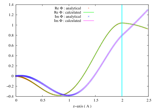
Figure 1: Real and imaginary part of the numerical solution of the SE along $z$ direction for the separable truncated potential given in the text, compared to the analytical one. (Color online)

In order to test the reliability of the method also in the case of a potential which is not truncated but varies substantially in sign and magnitude inside the defining region, we show in Fig. 2 the same comparison for the Mathieu functions, solution of the separable SE with periodic boundary conditions

$$\left[\frac{d^{2}}{dx^{2}}+\frac{d^{2}}{dy^{2}}+\frac{d^{2}}{dz^{2}}\right]\psi(x,y,z)$$

$$=(-a_{x}-a_{y}-a_{z}+2q_{x}\cos 2x+2q_{y}\cos 2y+2q_{z}\cos 2z)\psi(x,y,z)$$ (22)

for the case where

$$q_{x}=1.0,\quad a_{x}=-0.455139,\qquad{\rm parity=even,\;period=\pi}$$

$$q_{y}=0.3,\quad a_{y}=-0.044566,\qquad{\rm parity=even,\;period=\pi}$$

$$q_{z}=1.0,\quad a_{z}=+1.859110,\qquad{\rm parity=even,\;period=2\pi}$$

The energy eigenvalue is E = 1.359405, $l_{max}=20$ and the number of surface points is given by 1730. For the convenience of the reader the Mathieu functions are described in  A. The number of radial mesh points was equal to 250. Also in this case we employed both methods of integration with a switch radius of $2.45\,$ au.

In general the minimum number of surface points is chosen according to the rule that to integrate exactly $\int d\Omega Y_{L}(\Omega)$ we need $\approx(l+1)^{2}/3$ points. [25] If we want to integrate the product of two Spherical Harmonics, $l$ should be the sum of the individual $l^{\prime}s$; the same for a product three, etc… So for the 3-d Numerov we need to integrate only a product of two functions whose expansions are both truncated to a certain $l_{\rm max}$, therefore the number of points is $(2l_{\rm max}+1)^{2}/3$, whereas for the truncated separable potential and the Mathieu functions we have the product of three functions (one for each space coordinate), so we need $(3l_{\rm max}+1)^{2}/3$ points. Moreover for the matrix Numerov method we again have $(3l_{\rm max}+1)^{2}/3$ due to the calculation of $V_{LL^{\prime}}$.

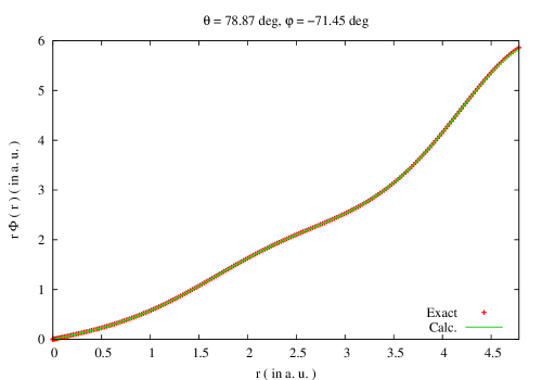
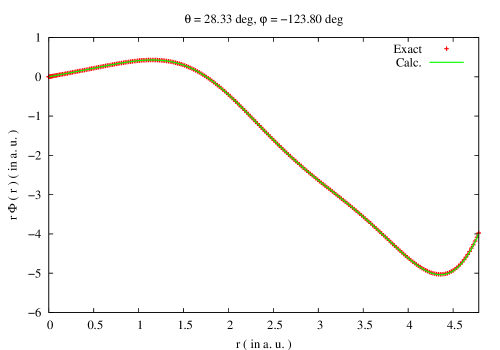
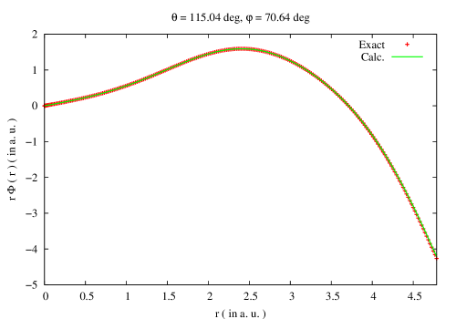
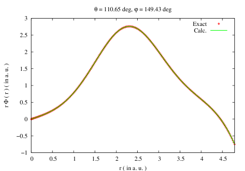
Figure 2: Comparison of the particular Mathieu function described in the text with the one generated by matrix and 3-d Numerov method at four different angles. The switch radius was at $2.45\,$ au. (Color online)

2.3 A linear-logarithmic mesh

To solve Eq. (1) by Numerov procedure, there are several choices for the radial mesh. Due to the singularity of the potential near the origin we found that the best strategy in our case was to take a mixed logarithmic and linear mesh, as usual in atomic physics.  [29, 30, 32] For non-MT calculation, especially with truncated potential, this mesh is the appropriate choice. In this case the new radial variable is

$$\rho\,(\,r\,)=\alpha\,r+\beta\,{\ln}\,r$$ (23)

with $\alpha$ and $\beta$ constant. A constant mesh size of $\rho$ can be taken in the interval $\rho_{0}\leq\rho\leq\rho_{N}$. The initial value of $\rho_{0}$ is chosen according to the empirical formula

$$\rho_{0}=-\beta\,(\,10+\,{\ln}\,Z\,)$$

whereas the final $\rho$ is defined as

$$\rho_{N}=\rho_{0}+Nh$$ (24)

so that $\alpha$ is given by

$$\alpha=(\rho_{N}-\beta\,{\ln}\,r_{N})/r_{N}$$ (25)

taking $\beta$, the mesh size $h$ and the number of points $N$ as input values. In the calculation of local basis functions we choose $r_{N}$ equal to the radius of the cell bounding sphere $R_{b}$, $\beta=1.0$ and put $N\approx 100R_{b}$. Instead for Fig.s 1 and 2 we took respectively $\beta=0.67$ and $\beta=0.05$. The value of $r=r(\rho)$ corresponding to a given value of $\rho$ can be readily found by application of the Newton technique. [32]

Following the change of variable in Eq. (23) the SE in Eq. (12) becomes ${\bf F}(\rho){\bf Y}(\rho)=0$ where

$$({\bf F}(\rho))_{LL^{\prime}}$$

$$=\Bigg{[}\left\{-\frac{d^{2}}{d\rho^{2}}+\left(\,\alpha+\frac{\beta}{r}\right)^{-2}\right.$$

$$\left.\times\left(\frac{l(l+1)+\beta\,(\,\alpha\,r+\beta/4\,)(\,\alpha\,r+\beta\,)^{-2}}{r^{2}}-E\right)\right\}\delta_{LL^{\prime}}$$

$$+\left(\,\alpha+\frac{\beta}{r}\right)^{-2}V_{LL^{\prime}}(r)\Bigg{]}$$

$${\bf Y}(\rho)=\sqrt{\alpha+\frac{\beta}{r}}\,{\bf X}\,(\,r\,)$$ (26)

where $r=r(\rho)$. The same, mutatis mutandis, applies to Eq. (1) for the three-dimensional Numerov method.

A comment is in order at this point. Strictly speaking by changing to the log-linear mesh the Eq.s (16-21) are not valid anymore, since $r=0$ cannot be realized (it would correspond to $\rho=-\infty)$ and therefore not explicitly implemented as boundary condition. By working out again the Gaussian elimination process when $X_{0}$ is not zero, one arrives at the same equations (20), except that in the rhs term the zero of the i-th row is replaced by $A_{i-1}\,D_{i-1}^{-1}\,A_{0}\,Y_{0}$, where $Y_{0}$ is the value of (26) calculated at the first point $\rho_{0}$. Now

$$Y_{LL^{\prime}}(\rho)=\sqrt{\alpha+{\beta\over r(\rho)}}X_{LL^{\prime}}(r(\rho))=\sqrt{\alpha r(\rho)+\beta}\sqrt{r(\rho)}R_{LL^{\prime}}(r(\rho))$$ (27)

Since at the origin $R_{LL^{\prime}}$ is diagonal in l and behaves like a spherical Bessel function, $\sqrt{r(\rho)}R_{LL}(r(\rho))$ is of the order of $10^{-3}$ for l=0 at $\rho_{0}\approx 10^{-5}$, $10^{-8}$ for l=1 etc.. We can therefore take $Y_{0}=0$ and use the simplified Gaussian elimination formulas Eq.s (16-21). We checked that this is a good approximation also for l=0.

3 Multiple scattering method for scattering and bound states

3.1 Scattering states

We begin by presenting the derivation of MSE for scattering states. In this case we seek a solution of the SE continuous in the whole space with its first derivatives, satisfying the asymptotic boundary condition

$$\psi({\bf r};{\bf k})\,\simeq\,\left(\frac{k}{16\pi^{3}}\right)^{\frac{1}{2}}\,\left[{\rm e}^{{\rm i}{\bf k}\cdot{\bf r}}+f(\hat{\bf r};{\bf k})\frac{{\rm e}^{{\rm i}{kr}}}{r}\right]$$ (28)

where ${\bf k}$ is the photo-electron wave-vector and $f(\hat{\bf r};{\bf k})$ is the scattering amplitude. The factor $\left(k/(16\pi^{3})\right)^{\frac{1}{2}}$ takes into account the normalization of the scattering states to one state per Ryd. In the spirit of MST we partition the space in terms of non overlapping space-filling cells $\Omega_{j}$ with surfaces $S_{j}$ and centers at ${\bf R}_{j}$. Accordingly we partition the overall space potential $V({\bf r})$ into cell potentials, such that $V({\bf r})=\sum_{j}v_{j}({\bf r}_{j})$, where $v_{j}({\bf r}_{j})$ takes the value of $V({\bf r})$ for ${\bf r}$ inside cell $j$ and vanishes elsewhere. As clear from the following the zero value of the potential outside the cell is not necessary and can be replaced by any constant. The results will not depend on this particular value. Here and in the following ${\bf r}_{j}={\bf r}-{\bf R}_{j}$. The partition is assumed to satisfy the requirement that the shortest inter-cell vector ${\bf R}_{ij}={\bf R}_{i}-{\bf R}_{j}$ joining the origins of the nearest neighbors cells $i$ and $j$, is larger than any intra-cell vector ${\bf r}_{i}$ or ${\bf r}_{j}$, when ${\bf r}$ is inside cell $i$ or cell $j$. If necessary, empty cells can be introduced to satisfy this requirement. We also assume that there exists a finite neighborhood around the origin of each cell lying in the domain of the cell. [12] We then start from the following identity involving surface integrals in ${d\hat{\bf r}}\equiv d\sigma$

$$\displaystyle{\sum_{j=1}^{N}\,\int_{S_{j}}\,\left[G_{0}^{+}({\bf r}^{\prime}-{\bf r};{\bf\kappa}){\bf\nabla}\psi({\bf r};{\bf k})-\psi({\bf r};{\bf k}){\bf\nabla}G_{0}^{+}({\bf r}^{\prime}-{\bf r};{\bf\kappa})\right]\cdot{\bf n}_{j}\,{\rm d}\sigma_{j}}$$

$$\displaystyle{=\int_{S_{o}}\,\left[G_{0}^{+}({\bf r}^{\prime}-{\bf r};{\bf\kappa}){\bf\nabla}\psi({\bf r};{\bf k})-\psi({\bf r};{\bf k}){\bf\nabla}G_{0}^{+}({\bf r}^{\prime}-{\bf r};{\bf\kappa})\right]\cdot{\bf n}_{o}\,{\rm d}\sigma_{o}\,}.$$ (29)

Here $\Omega_{o}=\sum_{j}\Omega_{j}$, with surface $S_{o}$, centered at the origin $o$ and $G_{0}^{+}({\bf r}^{\prime}-{\bf r};{\mathbf{\kappa}})$ is the free Green’s function with outgoing wave boundary conditions satisfying the equation $(\nabla^{2}+{\bf\kappa}^{2})\,G_{0}^{+}({\bf r}^{\prime}-{\bf r};{\bf\kappa})=\delta({\bf r}^{\prime}-{\bf r})$, where ${\bf\kappa}^{2}=E-V_{0}$ and $V_{0}$ is an arbitrary constant equal to the assumed value of the cell potential outside the cell domain. The identity (29)is valid for all ${\bf r}^{\prime}$ lying in the neighborhood of the origin of each cell, since in this case the integrands are continuous with their first derivatives. In this context we shall use two distinct $k$-vectors, defined respectively as ${k}=\sqrt{E}$ and ${\kappa}=\sqrt{E-V_{0}}$. This letter will appear in the expansion of the Green’s function $G_{0}^{+}({\bf r}^{\prime}-{\bf r};{\bf\kappa})$ by spherical functions.  [16] Obviously ${k}={\kappa}$ for $V_{0}=0$.

Equation (29), with the choice $V_{0}=0$, can also be derived from the Lippmann-Schwinger equation

$$\psi({\bf r}^{\prime};{\bf k})={\rm e}^{{\rm i}{\bf k}\cdot{\bf r}^{\prime}}+\int\,G_{0}^{+}({\bf r}^{\prime}-{\bf r};{k})\,V({\bf r})\,\psi({\bf r};{\bf k})\,{\rm d^{3}r}$$ (30)

satisfied by the scattering state (see C ). However we prefer to start from the identity Eq. (29) to take advantage of the arbitrariness of the constant $V_{0}$. For convenience of the reader we recall the expansions  [13]

$${\rm e}^{{\rm i}{\bf k}\cdot{\bf r}} = 4\pi\sum_{L}i^{l}Y_{L}(\hat{\bf k})J_{L}({\bf r};k)$$ (31)

$$G_{0}^{+}({\bf r}^{\prime}-{\bf r};{\bf\kappa}) = -\frac{1}{4\pi}\,\frac{e^{i{\bf\kappa}|{\bf r}^{\prime}-{\bf r}|}}{|{\bf r}^{\prime}-{\bf r}|}$$ (32)

$$= G_{0}^{+}({\bf r}_{i}^{\prime}-{\bf r}_{i};{\bf\kappa})$$

$$= \sum_{L}J_{L}({\bf r}_{i}^{\prime};{\bf\kappa})\tilde{H}_{L}^{+}({\bf r}_{i};{\bf\kappa})\;(r_{i}^{\prime}<r_{i})$$

$$= \sum_{L}J_{L}({\bf r}_{i};{\bf\kappa})\tilde{H}_{L}^{+}({\bf r}_{i}^{\prime};{\bf\kappa})\;(r_{i}^{\prime}>r_{i})$$ (33)

Notice for future reference that in the case ${\bf\kappa}=0$ the solid spherical harmonics $J_{L}({\bf r};{\bf\kappa})$ and $\tilde{H}_{L}^{+}({\bf r};{\bf\kappa})$ are to be understood as $\overline{J}_{L}({\bf r})=r^{l}Y_{L}(\hat{\bf r})/(2l+1)$ and $\overline{H}_{L}({\bf r})=r^{-l-1}Y_{L}(\hat{\bf r})$, due to the well known expansion

$$\frac{1}{|{\bf r}-{\bf r}^{\prime}|}=\sum_{L}\frac{4\pi}{2l+1}\,\frac{r_{<}^{l}}{r_{>}^{l+1}}\,Y_{L}(\hat{\bf r})\,Y_{L}(\hat{\bf r}^{\prime})$$ (34)

which is the $\kappa\rightarrow 0$ limit of Eq.s (32) and (33).

The heart of MST is the introduction of the functions $\Phi_{L}({\bf r}_{j};k)$ which inside cell $j$ are local solutions of the SE with potential $v_{j}({\bf r}_{j})$ behaving as $J_{L}({\bf r}_{j};k)$ for $r_{j}\rightarrow 0$. They form a complete set of basis functions such that the global scattering wave function can be locally expanded as  [12]

$$\psi({\bf r}_{j};{\bf k})=\sum_{L}A_{L}^{j}({\bf k})\Phi_{L}({\bf r}_{j};k)$$ (35)

where we have underlined the $k$ dependence of $\Phi_{L}({\bf r}_{j};k)$ through its behavior at the origin.

In order to find the asymptotic behavior in the outer region $\mathcal{C}\Omega_{o}$ we introduce the scattering functions in response to an exciting wave of angular momentum $L$:

$$\psi_{L}({\bf r}_{o};{k})=J_{L}({\bf r}_{o};k)+\int\,G_{0}^{+}({\bf r}_{o}-{\bf r}_{o}^{\prime};{k})\,V({\bf r}_{o}^{\prime})\,\psi_{L}({\bf r}_{o}^{\prime};{k})\,{\rm d^{3}r_{o}^{\prime}}$$ (36)

Then, under the assumption of short range potentials (i.e. potentials that behave like $1/r^{1+\epsilon}$ with positive $\epsilon$ at great distances), letting ${\bf r}_{o}\rightarrow\infty$ and using expansion Eq. (33) in Eq. (36) we find

$$\psi({\bf r}_{o};{\bf k}) = \sum_{L}\tilde{A}_{L}^{o}({\bf k})\Bigg{[}J_{L}({\bf r}_{o};k)$$ (37)

$$+\sum_{L^{\prime}}\tilde{H}_{L^{\prime}}^{+}({\bf r}_{o};k)\int J_{L^{\prime}}({\bf r}_{o}^{\prime};k)\,V({\bf r}_{o}^{\prime})\,\psi_{L}({\bf r}_{o}^{\prime};{k})\,{\rm d^{3}r_{o}^{\prime}}\Bigg{]}$$

$$= \sum_{L}\tilde{A}_{L}^{o}({\bf k})\Bigg{[}J_{L}({\bf r}_{o};k)+\sum_{L^{\prime}}\tilde{H}_{L^{\prime}}^{+}({\bf r}_{o};k)T_{L^{\prime}L}^{o}\Bigg{]}$$ (38)

where, in order to impose the asymptotic behavior in Eq. (28), $\tilde{A}_{L}^{o}=i^{l}Y_{L}(\hat{\bf k})\,({k/\pi})^{1/2}$ and $T_{LL^{\prime}}^{o}$ is the $T$-matrix for the whole cluster, equal to

$$T_{L^{\prime}L}^{o}=\int J_{L^{\prime}}({\bf r}_{o};k)\,V({\bf r}_{o})\,\psi_{L}({\bf r}_{o};{k})\,{\rm d^{3}r_{o}}$$ (39)

In general for short range potentials decaying slowly, the asymptotic behavior in Eq. (38) is reached only at great distance from the origin of the coordinates (usually at the center of the atomic cluster under study). In order to limit the number of cells, so that the surface $S_{o}$ just surrounds the cluster, we introduce the local solution

$$\Phi_{L}({\bf r}_{o};k)=\sum_{L^{\prime}}\,R_{L^{\prime}L}^{o}(r_{o})\,Y_{L^{\prime}}(\hat{\bf r}_{o})$$ (40)

in the outer region $\mathcal{C}\Omega_{o}$, which can be obtained by inward integration of the SE starting from the appropriate asymptotic value $\tilde{H}_{L^{\prime}}^{+}({\bf r}_{o};k)$. Therefore we take here

$$\psi({\bf r}_{o};{\bf k})=\sum_{L}\left[\tilde{A}_{L}^{o}({\bf k})J_{L}({\bf r}_{o};k)+\Phi_{L}({\bf r}_{o};k)A_{L}^{o}({\bf k})\right]$$ (41)

Notice that the function $\Phi_{L}({\bf r}_{o};k)$ in Eq. (40) (and consequently $R_{L^{\prime}L}^{o}(r_{o})$ ) is complex, unlike the functions $\Phi_{L}({\bf r}_{i};k)$ that can be taken real, if the potential is real. If the potential has a Coulomb tail, the spherical Bessel and Hankel functions should be replaced by the corresponding regular and irregular solutions $F_{L}({\bf r}_{o};k)$ and $G_{L}({\bf r}_{o};k)$ of the radial SE with a Coulomb potential. Due to the possibility that the optical potential used for calculating the spectroscopic response functions be complex, it should be clear from the context that the formalism works also for complex energies and/or potentials. The extension to complex energies will come very handy when exploiting the analytic properties of the Green function.

Insertion of the expressions Eq.s (35) and (41) into the identity Eq. (29) provides a set of algebraic equations (known as MSE) that determine the expansion coefficients $A^{j}_{L}({\bf k})$ and the $A_{L}^{o}({\bf k})$ in such a way that the local representations are smoothly continuous across the common boundary of contiguous cells. Indeed, taking ${\bf r}^{\prime}$ in the neighborhood of the origin of cell $i\neq o$, using the expansion Eq. (32) (since ${\bf r}$ is confined to lie on the cell surfaces), and putting to zero the coefficients of $J_{L}({\bf r}_{i}^{\prime};{\bf\kappa})$ due to their linear independence, we readily arrive at the MST compatibility equations for the amplitudes $A^{j}_{L}({\bf k})$ and $A_{L^{\prime}}^{o}({\bf k})$

$$\sum_{jL^{\prime}}H_{LL^{\prime}}^{ij}A^{j}_{L^{\prime}}({\bf k})=\sum_{L^{\prime}}\left[M_{LL^{\prime}}^{io}\tilde{A}_{L^{\prime}}^{o}({\bf k})+N_{LL^{\prime}}^{io}A_{L^{\prime}}^{o}({\bf k})\right]$$ (42)

where

$$H_{LL^{\prime}}^{ij}=\int_{S_{j}}[\,\tilde{H}_{L}^{+}({\bf r}_{i};\kappa)\nabla\Phi_{L^{\prime}}({\bf r}_{j};k)-\Phi_{L^{\prime}}({\bf r}_{j};k)\nabla\tilde{H}_{L}^{+}({\bf r}_{i};\kappa)\,]\cdot{\bf n}_{j}\,{\rm d}\sigma_{j}$$

$$M_{LL^{\prime}}^{io}=\int_{S_{o}}[\,\tilde{H}_{L}^{+}({\bf r}_{i};\kappa)\nabla J_{L^{\prime}}({\bf r}_{o};k)-J_{L^{\prime}}({\bf r}_{o};k)\nabla\tilde{H}_{L}^{+}({\bf r}_{i};\kappa)\,]\cdot{\bf n}_{o}\,{\rm d}\sigma_{o}$$

$$N_{LL^{\prime}}^{io}=\int_{S_{o}}[\,\tilde{H}_{L}^{+}({\bf r}_{i};\kappa)\nabla\Phi_{L^{\prime}}({\bf r}_{o};k)-\Phi_{L^{\prime}}({\bf r}_{o};k)\nabla\tilde{H}_{L}^{+}({\bf r}_{i};\kappa)\,]\cdot{\bf n}_{o}\,{\rm d}\sigma_{o}$$

A further set equation is obtained by taking ${\bf r}^{\prime}$ inside the outer region $\mathcal{C}\Omega_{o}$, using the expansion Eq. (33) (remembering that ${\bf r}_{o}<{\bf r}_{o}^{\prime}$, since ${\bf r}_{o}$ lies on $S_{o}$). By putting to zero the coefficients of $\tilde{H}_{L}^{+}({\bf r}_{o}^{\prime};{\bf\kappa})$ we obtain

$$\sum_{jL^{\prime}}K_{LL^{\prime}}^{oj}A^{j}_{L^{\prime}}({\bf k})=\sum_{L^{\prime}}\left[\tilde{M}_{LL^{\prime}}^{oo}\tilde{A}_{L^{\prime}}^{o}({\bf k})+\tilde{N}_{LL^{\prime}}^{oo}A_{L^{\prime}}^{o}({\bf k})\right]$$ (43)

where

$$K_{LL^{\prime}}^{oj}=\int_{S_{j}}[\,J_{L}({\bf r}_{o};\kappa)\nabla\Phi_{L^{\prime}}({\bf r}_{j};k)-\Phi_{L^{\prime}}({\bf r}_{j};k)\nabla J_{L}({\bf r}_{o};\kappa)\,]\cdot{\bf n}_{j}\,{\rm d}\sigma_{j}$$

$$\tilde{M}_{LL^{\prime}}^{oo}=\delta_{LL^{\prime}}\int_{S_{o}}[\,J_{L}({\bf r}_{o};\kappa)\nabla J_{L^{\prime}}({\bf r}_{o};k)-J_{L^{\prime}}({\bf r}_{o};k)\nabla J_{L}({\bf r}_{o};\kappa)\,]\cdot{\bf n}_{o}\,{\rm d}\sigma_{o}$$

$$\tilde{N}_{LL^{\prime}}^{oo}=\int_{S_{o}}[\,J_{L}({\bf r}_{o};\kappa)\nabla\Phi_{L^{\prime}}({\bf r}_{o};k)-\Phi_{L^{\prime}}({\bf r}_{o};k)\nabla J_{L}({\bf r}_{o};\kappa)\,]\cdot{\bf n}_{o}\,{\rm d}\sigma_{o}$$

From the above derivation it is clear that the set of equations in Eq.s (42) and (43) determines the amplitudes $A^{j}_{L}({\bf k})$ and $A_{L}^{o}({\bf k})$ independently of the constant $V_{0}$, since the identity Eq. (29) is valid whatever $V_{0}$. In general this will be true only if the $L$-expansion is not truncated, whereas there will be a more or less pronounced dependence according to the degree of convergence of the truncated expansion. In general, the lesser the potential jump at the boundaries of the various cells the faster the convergence.

Notice that these equations remain valid, with no restriction on the sums over $L$, even in the case $\kappa=0$, provided $J_{L}$ and $\tilde{H}_{L}$ are replaced by $\overline{J}_{L}$ and $\overline{H}_{L}$, due to the expansion Eq. (34) of the zero energy limit of the free Green’s Function.

The usual derivation of the MSE now proceeds by re-expanding $\tilde{H}_{L}^{+}({\bf r}_{i};\kappa)$ and $J_{L}({\bf r}_{o};\kappa)$ around center $j$ under the geometrical conditions stated at the beginning of this section, by use of the equations  [13, 16]

$$\tilde{H}_{L}^{+}({\bf r}_{i};\kappa)=\sum_{L^{\prime}}G^{ij}_{LL^{\prime}}J_{L^{\prime}}({\bf r}_{j};\kappa)\;(R_{ij}>r_{j})$$ (44)

$$J_{L}({\bf r}_{o};\kappa)=\sum_{L^{\prime}}J^{oj}_{LL^{\prime}}J_{L^{\prime}}({\bf r}_{j};\kappa)\;(\rm no\;cond.)$$ (45)

$$\tilde{H}_{L}^{+}({\bf r}_{i};\kappa)=\sum_{L^{\prime}}J^{io}_{LL^{\prime}}\tilde{H}_{L^{\prime}}^{+}({\bf r}_{o};\kappa)\;(r_{o}>R_{io})$$ (46)

where $G^{ij}_{LL^{\prime}}$ are the free electron propagator in the site and angular momentum basis ( KKR real space structure factors) given by

$$G^{ij}_{LL^{\prime}}=4\pi\sum_{L^{\prime\prime}}C(L,L^{\prime};L^{\prime\prime})\,i^{l-l^{\prime}+l^{\prime\prime}}\,\tilde{H}^{+}_{L^{\prime\prime}}({\bf R}_{ij};\kappa)$$ (47)

and $J^{ij}_{LL^{\prime}}$ is the translation operator

$$J^{ij}_{LL^{\prime}}=4\pi\sum_{L^{\prime\prime}}C(L,L^{\prime};L^{\prime\prime})\,i^{l-l^{\prime}+l^{\prime\prime}}\,J_{L^{\prime\prime}}({\bf R}_{ij};\kappa)$$ (48)

In these formulas the quantities $C(L,L^{\prime};L^{\prime\prime})$ are the real basis Gaunt coefficients given by

$$C(L,L^{\prime};L^{\prime\prime})=\int Y_{L}(\Omega)Y_{L^{\prime}}(\Omega)Y_{L^{\prime\prime}}(\Omega){\rm d}\Omega$$ (49)

In the following we shall also need the quantity

$$N^{ij}_{LL^{\prime}}=4\pi\sum_{L^{\prime\prime}}C(L,L^{\prime};L^{\prime\prime})\,i^{l-l^{\prime}+l^{\prime\prime}}\,N_{L^{\prime\prime}}({\bf R}_{ij};\kappa)$$ (50)

Unfortunately the re-expansions Eq.s (44), (45) and (46) introduce further expansion parameters into the theory (with related convergence problems) that are actually unnecessary, as shown below.

We in fact observe that the integrals over the surfaces of the various cells $j$ can be calculated over the surfaces of the corresponding bounding spheres (with radius $R_{b}^{j}$) by application of the Green’s theorem, since both $\tilde{H}_{L}^{+}({\bf r;\kappa})$ and $\Phi_{L}({\bf r;k})$ satisfy the Helmholtz equation $(\nabla^{2}+{\bf\kappa}^{2})\,F({\bf r})=0$ outside the domain of the cell. We then use the following relations

$$\int_{S_{j}}\,Y_{L^{\prime}}(\hat{\bf r}_{j})\,\tilde{H}_{L}^{+}({\bf r}_{i};\kappa)\,{\rm d}\sigma_{j}=(R_{b}^{j})^{2}\,G^{ij}_{LL^{\prime}}\,j_{l^{\prime}}(\kappa R_{b}^{j})$$ (51)

$$\int_{S_{j}}\,Y_{L^{\prime}}(\hat{\bf r}_{j})\nabla\,\tilde{H}_{L}^{+}({\bf r}_{i})\cdot{\bf n}_{j}\,{\rm d}\sigma_{j}=(R_{b}^{j})^{2}\,G^{ij}_{LL^{\prime}}\,\frac{\rm d}{{\rm d}R_{b}^{j}}\,j_{l^{\prime}}(\kappa R_{b}^{j})$$ (52)

which are exact for all $L$ provided $|{\bf r}_{i}-{\bf r}_{j}|=R_{ij}>r_{j}$ for ${\bf r}$ lying on the surface $S_{j}$. This is a consequence of the fact that under this condition the series in Eq. (44) converges absolutely and uniformly in the entire angular domain, as shown in B, Eq. (141) and can therefore be integrated term by term. This property is also true for the series derived with respect to ${\bf r}$. Even though not necessary, we also checked the numerical equality of both sides of Eq.s (51) and (52) for various values of $L,L^{\prime}$.

Similarly, since the series in Eq. (46) converges uniformly and absolutely, as shown in B, Eq. (142), we also find

$$\int_{S_{o}}\,Y_{L^{\prime}}(\hat{\bf r}_{o})\,\tilde{H}_{L}^{+}({\bf r}_{i};\kappa)\,{\rm d}\sigma_{j}=(R_{b}^{o})^{2}\,J^{io}_{LL^{\prime}}\,\tilde{h}_{l^{\prime}}^{+}(\kappa R_{b}^{o})$$ (53)

$$\int_{S_{o}}\,Y_{L^{\prime}}(\hat{\bf r}_{o})\nabla\,\tilde{H}_{L}^{+}({\bf r}_{i})\cdot{\bf n}_{j}\,{\rm d}\sigma_{j}=(R_{b}^{o})^{2}\,J^{io}_{LL^{\prime}}\,\frac{\rm d}{{\rm d}R_{b}^{o}}\,\tilde{h}_{l^{\prime}}^{+}(\kappa R_{b}^{o})$$ (54)

provided $R_{io}<R_{b}^{o}$, where $R_{b}^{o}$ is the bounding sphere of the outer region $\mathcal{C}\Omega_{o}$. Therefore $R_{b}^{o}$ should be bigger than any $R_{io}$.

Finally, due to the absolute and uniform convergence of the series in Eq. (45) without conditions, we find the following relations

$$\int_{S_{j}}\,Y_{L^{\prime}}(\hat{\bf r}_{j})\,J_{L}({\bf r}_{i};\kappa)\,{\rm d}\sigma_{j}=(R_{b}^{j})^{2}\,J^{ij}_{LL^{\prime}}\,j_{l^{\prime}}(\kappa R_{b}^{j})$$ (55)

$$\int_{S_{j}}\,Y_{L^{\prime}}(\hat{\bf r}_{j})\nabla\,J_{L}({\bf r}_{i})\cdot{\bf n}_{j}\,{\rm d}\sigma_{j}=(R_{b}^{j})^{2}\,J^{ij}_{LL^{\prime}}\,\frac{\rm d}{{\rm d}R_{b}^{j}}\,j_{l^{\prime}}(\kappa R_{b}^{j})$$ (56)

By inserting in Eq. (42) the expression for the basis functions expanded in spherical harmonics (we shall suppress the site indices whenever a relation refers to both sites $i$ and site $o$)

$$\Phi_{L}({\bf r};k)=\sum_{L^{\prime}}R_{L^{\prime}L}(r)Y_{L^{\prime}}(\hat{\bf r})$$ (57)

remembering that this expansion is uniformly convergent in the angular domain  [24] and using the relations Eq.s (51)-(56) we finally obtain, under the partitioning conditions specified at the beginning of Section 3,

$$\sum_{L^{\prime}}E_{LL^{\prime}}^{i}A^{i}_{L^{\prime}}({\bf k})\,+\sum_{j,L^{\prime},L^{\prime\prime}}^{j\neq i}G^{ij}_{LL^{\prime\prime}}S^{j}_{L^{\prime\prime}L^{\prime}}A^{j}_{L^{\prime}}({\bf k})$$

$$=\sum_{L^{\prime}}J^{io}_{LL^{\prime}}\left[M_{L^{\prime}L^{\prime}}^{oo}\tilde{A}_{L^{\prime}}^{o}({\bf k})+\sum_{L^{\prime\prime}}E_{L^{\prime}L^{\prime\prime}}^{o}A_{L^{\prime\prime}}^{o}({\bf k})\right]$$ (58)

where we have put $E_{L^{\prime}L^{\prime\prime}}^{o}\equiv N_{L^{\prime}L^{\prime\prime}}^{oo}$, the quantities $M_{LL}^{oo}$ and $N_{L^{\prime}L^{\prime\prime}}^{oo}$ being the same as those following Eq.(42), calculated with ${\bf r}_{i}$ replaced by ${\bf r}_{o}$.

Similarly, putting $S_{LL^{\prime}}^{o}\equiv\tilde{N}_{LL^{\prime}}^{oo}$, for Eq. (43) we find

$$\sum_{j,L^{\prime},L^{\prime\prime}}^{j\neq o}J^{oj}_{LL^{\prime\prime}}S^{j}_{L^{\prime\prime}L^{\prime}}A^{j}_{L^{\prime}}({\bf k})=\sum_{L^{\prime}}\left[\tilde{M}_{LL^{\prime}}^{oo}\tilde{A}_{L^{\prime}}^{o}({\bf k})\delta_{LL^{\prime}}+S_{LL^{\prime}}^{o}A_{L^{\prime}}^{o}({\bf k})\right]$$ (59)

In the above equations we have defined the quantities

$$E_{LL^{\prime}} = ({R_{b}})^{2}W[-i\kappa h_{l}^{+},R_{LL^{\prime}}]$$ (60)

$$S_{LL^{\prime}} = ({R_{b}})^{2}W[j_{l},R_{LL^{\prime}}]$$ (61)

for the cells $\Omega_{j}$ and for the outer region $\mathcal{C}\Omega_{o}$. The Wronskians $W[f,g]=fg^{\prime}-gf^{\prime}$ are calculated at $R_{b}^{j}$ and $R_{b}^{o}$ respectively and reduce to diagonal matrices for MT potentials.

Equations (58) and (59) look formally similar to the usual MSE. However we notice that due to the relations Eq.s (51)-(56) there are only two expansion parameters in the theory. They are related to the AM components of $R_{L^{\prime}L}$ in the expansion Eq. (57) in cell $j$ and in the outer region $\mathcal{C}\Omega_{o}$. No convergence constraints related to the re-expansion of the various spherical Bessel and Hankel functions around a different origin Eq.s (44)-(46) are present.

It is interesting to note that the truncation value for both indices is the same and corresponds to the classical relation $l_{\rm max}=kR_{b}^{j}$, where $R_{b}^{j}$ is the radius of the bounding sphere of the cell at site $j$. This is true for the index $L$, which reminds that the basis function $\Phi_{L}$ is normalized like $j_{l}(kr)Y_{L}$ near the origin. Due to the properties of the spherical Bessel functions, when $l\gg kR_{b}^{j}$, $\Phi_{L}$ becomes very small inside the cell, decreasing like $[(2l+1)!!]^{-1}$. Therefore his weight in the expansion Eq. (57) will be negligible. The other index $L^{\prime}$, as will be clear from the following, measures the response of the truncated potential inside the cell to an incident wave $J_{L^{\prime}}$ of angular momentum $L^{\prime}$. Due to the same argument as above, familiar to scattering theory, the scattering matrix $T_{L^{\prime}L}^{j}$ will decrease like $[(2l+1)!!(2l^{\prime}+1)!!]^{-1}$ (see Eq. (144) in B for $l,l^{\prime}\gg kR_{b}^{j}$). As a consequence $E^{j}$ and $S^{j}$ can be considered square matrices. In the case of the outer sphere region $\mathcal{C}{\Omega_{o}}$, the situation is inverted, the index $L$ being related to the response of the entire cluster to an incident wave of angular momentum $L$, whereas the index $L^{\prime}$ corresponds to the number of AM waves mixed in by the potential not only inside $\Omega_{o}$ but also in $\mathcal{C}\Omega_{o}$. The two indices have the same truncation $l_{\rm max}=k\tilde{R}_{b}^{o}$, provided we take $\tilde{R}_{b}^{o}$ as the radius of the sphere that contains the region of space where the potential is substantially different from zero. This conclusion is reinforced by the observation that one can cover this same region by empty cells.

Up to this point we have assumed that $V_{0}\neq 0$ and derived consequently the MSE, having in mind the possibility to check the rate of convergence of the $L$-expansion. However in the continuum case one usually works under the assumption that $V_{0}=0$. In this case the Eq.s (58) and (59) simplify considerably in the case of short range potentials. Since now $k=\kappa$, we use the relation

$$\int_{S_{o}}[\,\tilde{H}_{L^{\prime}}^{+}({\bf r}_{o};k)\nabla J_{L}({\bf r}_{o};k)-J_{L}({\bf r}_{o};k)\nabla\tilde{H}_{L^{\prime}}^{+}({\bf r}_{o};k)\,]\cdot{\bf n}_{j}\,{\rm d}\sigma_{o}=-\delta_{LL^{\prime}}$$ (62)

so that in Eq. (58) $M_{LL}^{oo}=-1$, and in Eq. (59) $\tilde{M}_{LL}^{oo}=0$. Moreover one easily finds that

$$\sum_{L^{\prime}}\tilde{A}_{L^{\prime}}^{o}({\bf k})J^{io}_{LL^{\prime}}=i^{l}Y_{L}({\bf k})\,e^{i{\bf k}\cdot{\bf R}_{io}}\sqrt{\frac{k}{\pi}}=I_{L}^{i}({\bf k})$$ (63)

which is obtained from Eq. (48) by observing that

$$\sum_{L^{\prime}}C(L,L^{\prime};L^{\prime\prime})Y_{L^{\prime}}(\Omega)=Y_{L}(\Omega)Y_{L^{\prime\prime}}(\Omega)$$

Then the two sets of equations assume the simpler form

$$\sum_{L^{\prime}}E_{LL^{\prime}}^{i}A^{i}_{L^{\prime}}({\bf k})\, +\sum_{j,L^{\prime},L^{\prime\prime}}^{j\neq i}G^{ij}_{LL^{\prime\prime}}S^{j}_{L^{\prime\prime}L^{\prime}}A^{j}_{L^{\prime}}({\bf k})$$ (64)

$$-\sum_{L^{\prime}L^{\prime\prime}}J^{io}_{LL^{\prime}}E_{L^{\prime}L^{\prime\prime}}^{o}A_{L^{\prime\prime}}^{o}({\bf k})=-I^{i}_{L}({\bf k})$$

$$\sum_{j,L^{\prime},L^{\prime\prime}}^{j\neq o}J^{oj}_{LL^{\prime\prime}}S^{j}_{L^{\prime\prime}L^{\prime}}A^{j}_{L^{\prime}}({\bf k})-\sum_{L^{\prime}}S_{LL^{\prime}}^{o}A_{L^{\prime}}^{o}({\bf k})=0$$ (65)

The fact that $E$ and $S$ can be taken to be square matrices leads to another interesting form of the MSE. Under the assumption that ${\rm Det}\,S\neq 0$, we can introduce new amplitudes

$$B_{L}({\bf k})=\sum_{L^{\prime}}S_{LL^{\prime}}A_{L^{\prime}}({\bf k})$$ (66)

which is equivalent to using new basis functions $\overline{\Phi}_{L}$ related to $\Phi_{L}$ by the relation

$$\overline{\Phi}_{L}=\sum_{L^{\prime}}(\tilde{S}^{-1})_{LL^{\prime}}\Phi_{L^{\prime}}$$ (67)

where $\tilde{S}$ is the transposed of the matrix $S$.

Defining the quantities

$$(T^{i})^{-1}=-E^{i}(S^{i})^{-1}$$ (68)

$$\overline{T}^{o}=-E^{o}(S^{o})^{-1}$$ (69)

(notice the asymmetry between sites $i$ and site $o$) we can write Eqs. (64) and (65) as

$$\sum_{L^{\prime}}(T^{i})_{LL^{\prime}}^{-1}B^{i}_{L^{\prime}}({\bf k})\, -\sum_{j,L^{\prime}}^{j\neq i}G^{ij}_{LL^{\prime}}B^{j}_{L^{\prime}}({\bf k})$$ (70)

$$-\sum_{L^{\prime}L^{\prime\prime}}J^{io}_{LL^{\prime}}\overline{T}^{o}_{L^{\prime}L^{\prime\prime}}B_{L^{\prime\prime}}^{o}({\bf k})=I^{i}_{L}({\bf k})$$

$$\sum_{j,L^{\prime}}^{j\neq o}J^{oj}_{LL^{\prime}}B^{j}_{L^{\prime}}({\bf k})-B^{o}_{L}({\bf k})=0$$ (71)

The meaning of the amplitudes $B_{L}({\bf k})$ is immediately found from these equations if we consider only a single truncated potential at center $i$. In this case $\overline{T}^{o}\equiv 0$, since now the asymptotic behavior is given by Eq. (38), and $B^{o}_{L}({\bf k})\equiv A_{L}^{o}({\bf k})=\sum_{L^{\prime}}T_{LL^{\prime}}^{o}\tilde{A}_{L^{\prime}}^{o}$ where $T_{LL^{\prime}}^{o}$ is the $T$-matrix of the potential. Therefore Eqs. (70) and (71) tell us that $T^{i}_{LL^{\prime}}\equiv T_{LL^{\prime}}^{o}$. As a consequence $B^{i}_{L}({\bf k})$ is the scattering amplitude of angular momentum $L$ in response to an exciting plane wave of wave vector ${\bf k}$. Moreover, we find that $T^{i}=-S^{i}(E^{i})^{-1}$ is symmetric in the AM indices (remember that we use a real spherical harmonics basis), a fact already known from general scattering theory. This is a consequence of the fact that $SE^{-1}$ is a symmetric matrix. [34]

In the case of many cells, it is expedient to work only in terms of the cell amplitudes $B^{i}_{L^{\prime}}({\bf k})$. Inserting into Eq. (70) the expression for $B^{o}_{L^{\prime}}({\bf k})$ given by Eq. (71) we obtain

$$\sum_{L^{\prime}}(T^{i})_{LL^{\prime}}^{-1}B^{i}_{L^{\prime}}({\bf k})\, -\sum_{j,L^{\prime}}^{j\neq i}G^{ij}_{LL^{\prime}}B^{j}_{L^{\prime}}({\bf k})$$ (72)

$$-\sum_{jL^{\prime}}\sum_{\Lambda\Lambda^{\prime}}J^{io}_{L\Lambda}\overline{T}^{o}_{\Lambda\Lambda^{\prime}}J^{oj}_{\Lambda^{\prime}L^{\prime}}B^{j}_{L^{\prime}}({\bf k})=I^{i}_{L}({\bf k})$$

Introducing $\tau$, the inverse of the multiple scattering matrix $M\equiv T^{-1}-G-J\overline{T}^{o}J$

$$\tau=(T^{-1}-G-J\overline{T}^{o}J)^{-1}$$ (73)

known as the scattering path operator [13], we derive from Eq. (72) that

$$B^{i}_{L}({\bf k})=\sum_{jL^{\prime}}\tau_{LL^{\prime}}^{ij}I^{j}_{L^{\prime}}({\bf k})$$ (74)

If we insert this expression in Eq. (71) and remember that by definition $B^{o}_{L}({\bf k})=\sum_{L^{\prime}}T_{LL^{\prime}}^{o}\tilde{A}_{L^{\prime}}^{o}$, we easily find for the cluster $T$-matrix

$$T_{LL^{\prime}}^{o}=\sum_{ij}\sum_{\Lambda\Lambda^{\prime}}J^{oi}_{L\Lambda}\tau_{\Lambda\Lambda^{\prime}}^{ij}J^{jo}_{\Lambda^{\prime}L^{\prime}}$$ (75)

Since the matrices $G$ and $J$ are also symmetric (see definitions Eq.s (47) and (48)), we find that $\tau$ is likewise symmetric, implying the symmetry of $T_{L^{\prime}L}^{o}$, again in keeping with scattering theory. This quantity represents indeed for the whole cluster the scattering amplitude into a spherical wave of angular momentum $L$ in response to an exciting wave of AM $L^{\prime}$ and is needed for example in electron molecular scattering. [33] Finally Eq. (74) shows that the quantities $B^{i}_{L}({\bf k})$ are scattering amplitudes for the cluster, for which the generalized optical theorem holds (for real potentials)  [33, 16] (see D)

$$\int{\rm d}\hat{\bf k}\,B^{i}_{L}({\bf k})\,\left[B^{j}_{L^{\prime}}({\bf k})\right]^{\ast}=-\frac{1}{\pi}\,\Im\,\tau_{LL^{\prime}}^{ij}$$ (76)

This relation is very important, since it establishes the connection between the photo-emission and the photo-absorption cross section, as shown in E. As it will turn out, $-\Im\,\tau_{LL}^{ii}$ is proportional to the $L$-projected density of states onto site $i$.

In the case of one single cell located at site $i$, by construction the solutions inside and outside the cell are continuously smooth so that, remembering that by definition $T^{i}_{LL^{\prime}}\equiv T_{LL^{\prime}}^{o}$, for $r_{i}=r_{o}=R_{b}^{i}$ we have, neglecting for simplicity from now on the $k$ dependence of the local solutions,

$$\sum_{L}B^{i}_{L}({\bf k})\overline{\Phi}_{L}({\bf r}_{i})=\sum_{L}\tilde{A}_{L}^{o}({\bf k})\left[J_{L}({\bf r}_{o};k)+\sum_{L^{\prime}}\tilde{H}_{L^{\prime}}^{+}({\bf r}_{o};k)T_{L^{\prime}L}^{i}\right]$$ (77)

Using Eq. (74) for a single site and equating the coefficients of $\tilde{A}_{L}^{o}({\bf k})$ we find at the bounding sphere the relation

$$\sum_{L^{\prime}}\overline{\Phi}_{L^{\prime}}({\bf r}_{i})T_{L^{\prime}L}^{i} = \sum_{L^{\prime}}(\tilde{E})_{LL^{\prime}}^{-1}\Phi_{L^{\prime}}$$ (78)

$$\equiv \underline{\Phi}_{L}$$

$$= J_{L}({\bf r}_{o};k)+\sum_{L^{\prime}}\tilde{H}_{L^{\prime}}^{+}({\bf r}_{o};k)T_{L^{\prime}L}^{i}$$

implying that the basis functions $\underline{\Phi}_{L}$ are scattering functions, obeying the Lippmann-Schwinger equation for the cell potential. Therefore, introducing new expansion coefficients $C_{L}({\bf k})$ such that locally

$$\psi({\bf r};{\bf k})=\sum_{L}C_{L}({\bf k})\underline{\Phi}_{L}({\bf r})$$ (79)

and repeating the steps leading to the MSE in this new basis, we obtain

$$C^{i}_{L}({\bf k})\,-\sum_{j,L^{\prime}L^{\prime\prime}}^{j\neq i}G^{ij}_{LL^{\prime\prime}}T_{L^{\prime\prime}L^{\prime}}^{j}C^{j}_{L^{\prime}}({\bf k})-\sum_{L^{\prime}}J^{io}_{LL^{\prime}}C_{L^{\prime}}^{o}({\bf k})=I^{i}_{L}({\bf k})$$ (80)

$$\sum_{j,L^{\prime}L^{\prime\prime}}^{j\neq o}J^{oj}_{LL^{\prime\prime}}T_{L^{\prime\prime}L^{\prime}}^{j}C^{j}_{L^{\prime}}({\bf k})=\sum_{L^{\prime}}(\overline{T}^{o})_{LL^{\prime}}^{-1}C_{L^{\prime}}^{o}({\bf k})$$ (81)

Comparing these equations with the previous ones in Eqs. (70), (71) and (64), (65) we immediately find the relations

$$B^{j}_{L}({\bf k}) = \sum_{L^{\prime}}T_{LL^{\prime}}^{j}C^{j}_{L^{\prime}}({\bf k})$$ (82)

$$B^{o}_{L}({\bf k}) = \sum_{L^{\prime}}(\overline{T}^{o})_{LL^{\prime}}^{-1}C_{L^{\prime}}^{o}({\bf k})$$ (83)

$$C_{L}({\bf k}) = \sum_{L^{\prime}}E_{LL^{\prime}}A_{L^{\prime}}({\bf k})$$ (84)

In the present approach, the three forms of pair of equations (64)-(65), (70)-(71) and (80)- (81) are equivalent and lead to the same result.

The pair of equations (80)-(81) are quite important, since they provide the formal justification that in MST one can work with square matrices, provided that the only indexes appearing in the theory are those of the radial functions $R_{LL^{\prime}}(r)$. This is a consequence of the relation (143) of B (second equation) and the fact that the matrix elements $T_{LL^{\prime}}$ have a common truncation parameter $l_{\rm max}$. In fact, since $Tr(T^{\dagger}T)<\infty$ due to the asymptotic behavior of the $T_{LL^{\prime}}$ matrix elements given by Eq. (144) in the same Appendix, one can safely define an inverse for the matrix $T_{LL^{\prime}}(E)$ (except at poles on the negative energy axis) and pass from one representation to the other. In particular one can pass from the set (80)-(81) to the set (64)-(65). In the traditional derivation of MS equations, that does not rely on the relations (51)-(56) but hinges on the re-expansion formulas (44)-(46), this equivalence does not hold. In fact the need to saturate the ”internal” sum over $L^{\prime\prime}$ coming from the re-expansion introduces a further expansion parameter and therefore rectangular matrices into the theory. This feature makes it impossible to define a $T$-matrix and to write a closed form for the GF, loosing all the advantages of MST over other methods. This drawback has been avoided in our approach, since in each step of the derivation of the MS equations we have shown that the introduction of summation indices other than those present in the radial functions $R_{L^{\prime}L}(r)$ is unnecessary.

Another useful consequence of the fact that the theory can be cast in terms of square matrices is the possibility to exploit the point symmetry of the cluster under study. Even though many authors have treated the problem of how to symmetrize the MSE, this was done in the framework of the MT theory, where the cell T-matrices are diagonal in the AM indices. New features appear in the more general case (in particular how to calculate the symmetrized version of the $T_{LL^{\prime}}$ matrices) and F deals with this situation. Needless to say, we checked in all applications that the symmetrized and unsymmetrized version of the theory gave the same results. The application of the symmetrization procedure to Green’s Functions or to periodic systems is rather straightforward.

As already anticipated in the introduction, one of the major advantages of MST is the direct access to the Green’s Function of the system. Having explicit expressions for this quantity is of the utmost importance both for writing down spectroscopic response functions (see Ref. [35]) and for the calculation of ground state properties through contour integration in the complex energy plane (see e.g. Ref. [9] and references therein).

The GF is solution of the Schrödinger equation with a source term

$$(\nabla^{2}\,+E-V\,({\bf r})\,)\,G({\bf r},{\bf r}^{\prime};E)=\delta({\bf r}-{\bf r}^{\prime}).$$ (85)

In the framework of MST and for general (possibly complex) potentials, the solution of this equation in the case of a finite cluster can be written as  [13, 36]

$$G({\bf r}_{i},{\bf r}_{j}^{\prime};E) = \,\langle\,\overline{\Phi}({\bf r}_{i})\,|\,(\,\tau^{ij}-\,\delta_{ij}\,T^{i}\,)\,|\,\overline{\Phi}({\bf r}_{j}^{\prime})\,\rangle$$ (86)

$$+ \,\delta_{ij}\,\langle\,\overline{\Phi}({\bf r}_{<})\,|\,T^{i}\,|\,{\Psi}({\bf r}_{>}^{\prime})\,\rangle$$

where ${\bf r}_{<}$ (${\bf r}_{>}$) indicates the lesser (the greater) between $r_{i}$ and $r_{i}^{\prime}$. The function ${\Psi}({\bf r})$ is the irregular solution in cell $i$ that matches smoothly to $\tilde{H}_{L^{\prime}}^{+}({\bf r})$ at $R_{b}^{i}$. For short we have saturated the sum over the angular momentum indices using a bra and ket notation (e. g.)

$$\langle\,\overline{\Phi}({\bf r}_{i})\,|\,\tau^{ij}|\,\overline{\Phi}({\bf r}_{j}^{\prime})\,\rangle=\sum_{LL^{\prime}}\overline{\Phi}_{L}({\bf r}_{i})\,\tau^{ij}_{LL^{\prime}}\,\overline{\Phi}_{L^{\prime}}({\bf r}_{j}^{\prime})$$ (87)

Moreover, for simplicity of presentation we have assumed no contribution from the outer region potential (i.e. $\overline{T}^{o}\equiv 0$) allowing empty cells to cover the volume $\Omega_{o}$ up to the point at which the asymptotic behavior in Eq. (38) starts to be valid. The modifications needed in the case $\overline{T}^{o}\neq 0$ are obvious. In the case of a crystal we have to work in Fourier space [9].

Now, from Eq. (78) written as

$$\overline{\Phi}_{L}({\bf r}_{i})=\sum_{L^{\prime}}J_{L^{\prime}}({\bf r}_{o};k)(T^{-1})_{L^{\prime}L}^{i}+\tilde{H}_{L}^{+}({\bf r}_{o};k)$$ (88)

by continuity we derive inside cell $i$ the relation

$$\underline{\Phi}_{L}({\bf r}_{i})=\sum_{L^{\prime}}\Lambda_{L^{\prime}}({\bf r}_{i};k)(T^{-1})_{L^{\prime}L}^{i}+\Psi_{L}({\bf r}_{i};k)$$ (89)

where $\Lambda_{L^{\prime}}({\bf r}_{i})$ is the irregular function joining smoothly to $J_{L^{\prime}}({\bf r}_{o};k)$ at $R_{b}^{i}$. Therefore the Green’s function takes the form

$$G({\bf r}_{i},{\bf r}_{j}^{\prime};E) = \,\langle\,\overline{\Phi}({\bf r}_{i})\,|\,\tau^{ij}\,|\,\overline{\Phi}({\bf r}_{j}^{\prime})\,\rangle$$ (90)

$$- \,\delta_{ij}\,\langle\,\overline{\Phi}({\bf r}_{<})\,|\,{\Lambda}({\bf r}_{>}^{\prime})\,\rangle$$

For real potentials, both $\overline{\Phi}_{L}$ and $\Lambda_{L}$ are real, so that the singular atomic term does not contribute to the imaginary part of the GF. In this case the quantity $-\Im\,\int_{\Omega_{i}}\,G({\bf r},{\bf r};E)\,{\rm d^{3}}r=-\sum_{L}\,\Im\,\tau_{LL}^{ii}\,(E)\,\int_{\Omega_{i}}\overline{\Phi}_{L}^{2}({\bf r})\,{\rm d^{3}}r$ is the projected density of states on site $i$ at energy $E$, expressed as a sum of the partial densities of type $L$. This relation (not ${\bf r}$-integrated) constitutes the basis for calculating the system density by contour integration in the complex energy plane.

Alternative forms of the GF that are independent of the normalization of the local solutions $\Phi_{L}({\bf r}_{i})$ can be easily obtained in terms of the $S$ and $E$ matrix. For example we have

$$G({\bf r}_{i},{\bf r}_{j}^{\prime};E)$$

$$=-\,\langle\,\Phi({\bf r}_{i})\,|\,\,\{([\,\tilde{S}\,E+\tilde{S}G\,S\,]^{-1})^{ij}-\delta_{ij}\,([\,\tilde{S}\,E\,]^{-1})^{ii}\,\}\,|\,\Phi({\bf r}_{j}^{\prime})\,\rangle$$

$$-\,\delta_{ij}\,\langle\,\Phi({\bf r}_{<})\,|\,E^{-1}\,|\,{\Psi}({\bf r^{\prime}}_{>})\,\rangle$$ (91)

which is seen to reduce to the following expression, remembering the definition of $|\,\underline{\Phi}\,\rangle$,

$$G({\bf r}_{i},{\bf r}_{j}^{\prime};E) = \,\langle\,\underline{\Phi}({\bf r}_{i})\,|\,(\,[\,I-\,G\,T\,]^{-1}\,G\,)^{ij}\,\,|\,\underline{\Phi}({\bf r}_{j}^{\prime})\,\rangle$$ (92)

$$- \,\delta_{ij}\,\langle\,\underline{\Phi}({\bf r}_{<})\,|\,{\Psi}({\bf r^{\prime}}_{>})\,\rangle$$

Indeed from the relation,

$$(A+B)^{-1}-A^{-1} = (A+B)^{-1}\,(A-(A+B))\,{A}^{-1}$$ (93)

$$= -(A+B)^{-1}BA^{-1}$$

$$= -(B^{-1}A+1)^{-1}A^{-1}$$

$$= -(AB^{-1}A+A)^{-1}$$

we find

$$[\,\tilde{S}\,E+\tilde{S}\,G\,S\,]^{-1}-[\,\tilde{S}\,E\,]^{-1} = -[\,\tilde{S}\,E+\,\tilde{S}\,E\,[\,\tilde{S}\,G\,S\,]^{-1}\,\tilde{S}\,E\,]^{-1}$$ (94)

$$= -[\,\tilde{S}\,E+\,\tilde{S}\,E\,[\,G\,S\,]^{-1}\,E\,]^{-1}$$

$$= -\,E^{-1}\,[\,\tilde{S}+\,\tilde{S}\,E\,[\,G\,S\,]^{-1}\,]^{-1}$$

$$= -\,E^{-1}\,[\,\tilde{S}+\,\tilde{E}\,S\,[\,G\,S\,]^{-1}\,]^{-1}\,$$

$$= \,E^{-1}\,[\,T-G^{-1}\,]^{-1}\,\tilde{E}^{-1}$$

$$= \,-E^{-1}\,[\,I-G\,T\,]^{-1}\,G\,\tilde{E}^{-1}$$

taking into account that $\tilde{S}\,E\,=\tilde{E}\,S\,$ and $T=-SE^{-1}=-\tilde{E}^{-1}\tilde{S}$. All these forms are equivalent as long as we can treat the matrices $S$ and $E$ as square.

3.2 Bound states

Even though the essential of this section has been presented in a conference proceedings  [22], we feel that for the sake of completeness of presentation and convenience of the reader it should be repeated here.

The MSE in the case of bound states can be derived from those for scattering states, by simply eliminating the exciting plane wave in Eq. (106) and taking the analytical continuation to negative energies in free Green’s function $G_{0}^{+}({\bf r}^{\prime}-{\bf r};k)$, in order to impose the boundary condition of decaying waves when $r^{\prime}\rightarrow\infty$. In this case the Lippmann-Schwinger equation reduces to the eigenvalue equation

$$\psi({\bf r}^{\prime})=\int\,G_{0}^{+}({\bf r}^{\prime}-{\bf r};k)\,V({\bf r})\,\psi({\bf r})\,{\rm d^{3}r}$$ (95)

where we have dropped the label ${\bf k}$ in the wave function $\psi({\bf r}^{\prime})$. Since the expansion of $G_{0}^{+}({\bf r}^{\prime}-{\bf r};k)$ in terms of spherical Bessel and Hankel functions in Eqs. (32) and (33) remain valid under the analytical continuation to negative energies, so that $k=\sqrt{E}=i\sqrt{|E|}=i\gamma$, we see that $\psi({\bf r}^{\prime})$ behaves like $e^{ikr^{\prime}}/r^{\prime}=e^{-\gamma r^{\prime}}/r^{\prime}$ for $r^{\prime}\rightarrow\infty$. We remind that

$$h_{l}^{+}(kr)=-{i}^{-l}\,K_{l}^{1}(\gamma r); h_{l}^{-}(kr)=-{i}^{-l}(-1)^{l}\,K_{l}^{2}(\gamma r)$$

$$j_{l}(kr)={i}^{l}\,I_{l}(\gamma r); n_{l}(kr)=i^{l+1}\frac{(-1)^{l+1}K_{l}^{1}+K_{l}^{2}}{2}$$ (96)

where $I_{l}$ is the modified Bessel and $K_{l}^{1}$, $K_{l}^{2}$ the modified Hankel functions of first and second kind, respectively. Not only the expansions in Eqs. (32) and (33), but also the re-expansion relations in Eqs. (44), (45) and (46) remain valid under analytical continuation with the same convergence properties (see B). This fact implies that we can derive the MSE for bound states following the same patterns as for scattering states, except that now the behavior of the wave function in the outer region $\mathcal{C}\Omega_{o}$ is

$$\psi({\bf r}_{o}) = \sum_{L}A_{L}^{o}\,\Phi_{L}^{o}({\bf r}_{o})$$ (97)

$$= \sum_{L}A_{L}^{o}\,\sum_{L^{\prime}}\,R_{L^{\prime}L}^{o}(r_{o})\,Y_{L^{\prime}}(\hat{\bf r}_{o})$$

The functions $\Phi_{L}^{o}({\bf r}_{o})$ are now real and can easily be found by inward integration in the outer region starting from an asymptotic WKB solution properly normalized, e.g. like $[(2l+1)!!]^{-1}$.

Working with the $B_{L}$ amplitudes we easily arrive at the following condition for the existence of a bound state

$$\sum_{jL^{\prime}}\left\{(T^{i})_{LL^{\prime}}^{-1}\delta_{ij}\,-(1-\delta_{ij})\,G^{ij}_{LL^{\prime}}-\sum_{L^{\prime}L^{\prime\prime}}J^{io}_{LL^{\prime}}\overline{T}_{L^{\prime}L^{\prime\prime}}^{o}J^{oj}_{L^{\prime\prime}L^{\prime}}\right\}B^{j}_{L^{\prime}}=0$$ (98)

which is the same as Eq. (72), except that the exciting plane wave term $I^{i}_{L}({\bf k})$ and the ${\bf k}$ dependence have been dropped. Notice that we have kept the arbitrariness of $V_{0}$ in the free Green’s function, in order to check that the eigenvalues do not depend on it. In the spirit of the analytical continuation, we have a definite rule on how to calculate the various quantities as a function of $\kappa$.

We now define

$$C_{LL^{\prime}}=({R_{b}})^{2}W[n_{l},R_{LL^{\prime}}]$$ (99)

so that, remembering Eq. (69)

$$\kappa^{-1}(T^{j})^{-1}=(K^{j})^{-1}+i=-C^{j}(S^{j})^{-1}+i$$ (100)

$$\kappa^{-1}\overline{T}^{o}=\overline{K}^{o}+i=-C^{o}(S^{o})^{-1}+i$$ (101)

Moreover we observe that

$$\kappa^{-1}G^{ij}_{LL^{\prime}}=N^{ij}_{LL^{\prime}}-iJ^{ij}_{LL^{\prime}}$$ (102)

where $N^{ij}_{LL^{\prime}}$ is defined in Eq. (50) and that $\sum_{L^{\prime\prime}}J^{io}_{LL^{\prime\prime}}J^{oj}_{L^{\prime\prime}L^{\prime}}=J^{ij}_{LL^{\prime}}$, since $J$ is the translational operator. Substituting these relations into Eq. (98) and eliminating the common factor $\kappa^{-1}$ we finally find

$$\sum_{jL^{\prime}}\left\{(K^{i})_{LL^{\prime}}^{-1}\delta_{ij}\,-(1-\delta_{ij})\,N^{ij}_{LL^{\prime}}-\sum_{L^{\prime}L^{\prime\prime}}J^{io}_{LL^{\prime}}\overline{K}_{L^{\prime}L^{\prime\prime}}^{o}J^{oj}_{LL^{\prime}}\right\}B^{j}_{L^{\prime}}=0$$ (103)

The generic ($LL^{\prime}$)-element of this MS matrix is either real for real $\kappa$ ($E-V_{0}>0$) or proportional to $i^{l-l^{\prime}+1}$ for imaginary $\kappa$ ($E-V_{0}<0$). Indeed, due to the relations Eq. (96), putting for short $K_{l}=[(-1)^{l+1}K_{l}^{1}+K_{l}^{2}]/2$, we easily find that

$$N_{LL^{\prime}} = 4\pi i^{l-l^{\prime}+1}\sum_{L^{\prime\prime}}C(L,L^{\prime};L^{\prime\prime})\,(-1)^{l^{\prime\prime}}\,K_{l^{\prime\prime}}(|\kappa|R_{ij})Y_{L^{\prime\prime}}({\bf R}_{ij})$$

$$(K^{i})_{LL^{\prime}}^{-1} = -i^{l-l^{\prime}+1}\left[\underline{C}^{i}(\underline{S}^{i})^{-1}\right]_{LL^{\prime}}$$

$$\overline{K}_{LL^{\prime}}^{o} = -i^{l-l^{\prime}+1}\left[\underline{C}^{o}(\underline{S}^{o})^{-1}\right]_{LL^{\prime}}$$

where $\underline{C}$ and $\underline{S}$ are defined in terms of the modified spherical Bessel and Neumann functions as the corresponding quantities.

Therefore the condition for a bound state becomes ${\rm Det}\,\underline{M}=0$, where $\underline{M}$ is the MS matrix in Eq. (103) after a unitary transformation that eliminates the imaginary factors. In the practical numerical implementation we find the zeros of the determinant of ${\rm Det}\,(K\underline{M})$, excluding the spurious solutions coming from the zeros of ${\rm Det}\,\underline{S}$. In this form, the procedure is equivalent to finding the poles of the GF in the form Eq. (92) on the real negative axis, as it should be. Still numerical instabilities might come from the inverse of $\underline{S}^{o}$ present in the contribution of the outer sphere region. This unwanted feature could be eliminated by working with the $A_{L}$, instead of the $B_{L}$ amplitudes.

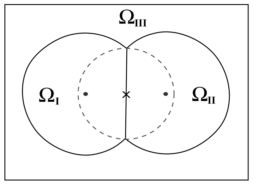
Figure 3: Partitioning of the space for the hydrogen molecular ion with no empty cells.

Table 1: Eigenvalues of the hydrogen molecular ion (in Ryd)

Mol. orb.	n l m	Exact	Smith & Johnson[37]	Foulis [34]	22 EC V0=-1.90	22 EC V0= 0	No EC V0=-1.90	No EC V0= 0
1a1g	1 0 0	-2.20525	-2.0716	-2.18973	-2.20522	-2.2055	-2.2050	-2.2048
2a1g	2 0 0	-0.72173	-0.70738	-0.72093	-0.723	-0.724	-0.731	-0.726
3a1g	3 2 0	-0.47155	-0.45574	-0.47102	-0.4727	-0.478	-0.476	-0.474
4a1g	3 0 0	-0.35536	-0.34859	-0.35525	-0.356	-0.3550	-0.357	-0.356
1a2u	2 1 0	-1.33507	-1.2868	-1.33426	-1.3348	-1.3348	-1.3342	-1.3343
2a2u	3 1 0	-0.51083	-0.49722	-0.51085	-0.51072	-0.5105	-0.5104	-0.5104
3a2u	4 1 0	-0.27463	-0.26979	-0.27466	-0.27469	-0.2742	-0.2745	-0.2745
4a2u	4 3 0	-0.25329	-0.24997	-0.25329	-0.254	-0.2536	-0.2541	-0.25301
1e1g	3 2 1	-0.45340	-0.44646	-0.45333	-0.4545	-0.45332	-0.455	-0.455
1e1u	2 1 1	-0.85755	-0.88866	-0.85585	-0.85754	-0.8561	-0.870	-0.858

We applied the theory above to find the exact eigenvalues of the hydrogen molecular ion, since this test is considered rather stringent for the validity of the theory due to rapid variation of the potential in the molecular region and to the awkward geometry of the cells. In this case we partition the space in three regions, as illustrated in Fig. 3, two truncated spheres around the protons with a radius of 1.72 a.u. corresponding to cells $\Omega_{I}$ and $\Omega_{II}$ and an external region labeled $\Omega_{III}$, corresponding to the complementary domain $\mathcal{C}\Omega_{o}$. The bounding sphere of this latter is represented by the dashed circle with radius 1.4 a.u., bigger than one half the distance of the protons, as discussed after Eq. (54). By calling the region outside this circle $\mathcal{C}\Omega_{b}$, the potential is taken to be zero (or constant) into the intersection of this domain with cells $\Omega_{I}$ and $\Omega_{II}$, and equal to the value of the true potential in the intersection with $\mathcal{C}\Omega_{o}$. We also did a calculation with the two atomic cells, 22 empty cells surrounding them, plus an external region.

It should be noticed that treatment of bound state is done here in analogy to the X-$\alpha$ MST method [3], since we intend to put the theory to a severe test concerning the independence of the eigenvalues from the value of the interstitial constant $V_{0}$ and the partitioning of the space. More modern techniques that avoid finding eigenvalues and eigenstates of the molecular cluster in the course of a SCF-iteration, exploit the analyticity of the GF through a contour integration in the complex energy plane to find directly the molecular density, as mentioned in the introduction and in Section 3.1.

Our findings are listed into Table (1) and compared with the exact results. The last two columns show the eigenvalues obtained with two different values of $V_{0}$, respectively equal to -1.90 Ryd and 0, showing the ’quasi’ independence of the results from the constant interstitial value $V_{0}$. The columns with the label ’22 EC’ refer to the calculation with two atomic cells, 22 empty cells and an external region, showing the ’quasi’ independence of the result from the partitioning mode of the space. We attribute the slight dependence of the eigenvalues on $V_{0}$ and the partitioning mode to the numerical instabilities mentioned above and the $L$-truncation of the matrices.

The column labeled ’Smith & Johnson’ refers to the calculation by Smith and Johnson [37] in the MT approximation, whereas the one labeled ’Foulis’ quotes the result by Foulis [34] obtained within the distorted wave approximation.

4 Convergence of Full Potential Multiple Scattering Theory

The inversion of the MS matrix becomes computationally heavy at high photoelectron energies because of the large number of angular momenta involved, since $l_{\rm max}\approx kR_{b}$. A common way to circumvent this difficulty is to invert the MS matrix by series, whereby

$$(T^{-1}-G)^{-1}=T\,\sum_{n}(GT)^{n}.$$ (104)

While this series is absolutely convergent for nonoverlapping MT spheres, provided the spectral radius of the matrix $GT$ is less than one [38], it is known to diverge for the case of space-filling cells. This is easily seen by using the inequality (145) in B, putting $l=l^{\prime}\gg l_{\rm max}$, whereby

$$|G_{ll}T_{ll}|\approx R_{b}\,\bigg{(}\frac{2R_{b}}{R_{ij}}\bigg{)}^{2l+1}$$ (105)

which signals the divergence of the matrix element $(GT)_{ll}$ (for space-filling cells $2R_{b}>R_{ij}$, at least for nearest neighbors).

However due to the behavior shown by Eq. (105) there is a widespread belief that the procedure of inverting exactly an $l$ truncated MS matrix and then letting $l$ go to $\infty$ does not converge in the case of space-filling cells. We shall show in the following that this is not so, provided a slight modification of the free propagator $G$ is adopted.

In order to illustrate our point, let us start by solving the Lippmann-Schwinger equation using the theory of the integral equations, before applying MST.

$$\psi({\bf r}^{\prime};{\bf k})={\rm e}^{{\rm i}{\bf k}\cdot{\bf r}^{\prime}}+\int\,G_{0}^{+}({\bf r}^{\prime}-{\bf r};{k})\,V({\bf r})\,\psi({\bf r};{\bf k})\,{\rm d^{3}r}$$ (106)

We cannot use Fredholm theory, since the Kernel for this integral equation

$${\bf K}({\bf r}^{\prime},{\bf r})=-\frac{1}{4\pi}\,\frac{{\rm e}^{{\rm i}{\bf k}\cdot|{\bf r}^{\prime}-{\bf r}|}}{|{\bf r}^{\prime}-{\bf r}|}\,V({\bf r})$$ (107)

is such that

$$Tr({\bf K}^{\dagger}{\bf K}) = \,\int\int{\rm d}{\bf r}{\rm d}{\bf r}^{\prime}\,{\bf K}^{\star}({\bf r}^{\prime},{\bf r})\,{\bf K}({\bf r}^{\prime},{\bf r})$$ (108)

$$= \left({\frac{1}{4\pi}}\right)^{2}\,\int\int{\rm d}{\bf r}{\rm d}{\bf r}^{\prime}\,\frac{V({\bf r})^{2}}{|{\bf r}^{\prime}-{\bf r}|^{2}}$$

$$\leq \left({\frac{1}{4\pi}}\right)^{2}\,\int\int{\rm d}{\bf r}{\rm d}{\bf r}^{\prime}\,\frac{|V({\bf r})|^{2}}{|{\bf r}^{\prime}-{\bf r}|^{2}}$$

and obviously diverges.

However a solution for this problem can be found by following the argument of section 10.3, page 280 of Ref. 39 in the paper (Newton). We multiply the Lippmann-Schwinger equation Eq. (106) by $|V({\bf r}^{\prime})|^{1/2}$ and write $V({\bf r})=|V({\bf r})|v({\bf r})$, where $v({\bf r})$ is a sign factor, equal to $+1$ where the potential is positive and to $-1$ where it is negative. Then we obtain

$$\psi_{s}({\bf r}^{\prime};{\bf k}) \equiv |V({\bf r}^{\prime})|^{1/2}\,\psi({\bf r}^{\prime};{\bf k})$$ (109)

$$= |V({\bf r}^{\prime})|^{1/2}\,{\rm e}^{{\rm i}{\bf k}\cdot{\bf r}^{\prime}}$$

$$+ |V({\bf r}^{\prime})|^{1/2}\,\int\,G_{0}^{+}({\bf r}^{\prime}-{\bf r};{k})\,|V({\bf r})|^{1/2}\,v({\bf r})\,\psi_{s}({\bf r};{\bf k})\,{\rm d^{3}r}$$

The Kernel for this integral equation is given by

$${\bf K}_{s}({\bf r}^{\prime},{\bf r})=-\frac{1}{4\pi}\,|V({\bf r}^{\prime})|^{1/2}\,\frac{{\rm e}^{{\rm i}{\bf k}\cdot|{\bf r}^{\prime}-{\bf r}|}}{|{\bf r}^{\prime}-{\bf r}|}\,|V({\bf r})|^{1/2}\,v({\bf r})$$ (110)

whereby

$$Tr({\bf K}_{s}^{\dagger}{\bf K}_{s}) = \,\int\int{\rm d}{\bf r}{\rm d}{\bf r}^{\prime}\,{\bf K}^{\star}({\bf r}^{\prime},{\bf r})\,{\bf K}({\bf r}^{\prime},{\bf r})$$ (111)

$$= \left({\frac{1}{4\pi}}\right)^{2}\,\int\int{\rm d}{\bf r}{\rm d}{\bf r}^{\prime}\,\frac{V({\bf r})\,|V({\bf r}^{\prime})|}{|{\bf r}^{\prime}-{\bf r}|^{2}}$$

$$\leq \left({\frac{1}{4\pi}}\right)^{2}\,\int\int{\rm d}{\bf r}{\rm d}{\bf r}^{\prime}\,\frac{|V({\bf r})|\,|V({\bf r}^{\prime})|}{|{\bf r}^{\prime}-{\bf r}|^{2}}$$

which is finite for a large class of potentials (including the molecular ones), so that the kernel ${\bf K}_{s}$ is of the Hilbert-Schmidt type and Fredholm theorem for $L_{2}$-kernels can be applied. Once the solution $\psi_{s}({\bf r}^{\prime};{\bf k})$ is found, we can obtain the solution of Eq. (106) simply by dividing it by $|V({\bf r}^{\prime})|^{1/2}$, except at points for which $|V({\bf r}^{\prime})|^{1/2}=0$, where it can be defined by continuity.

Now, let us apply MST to Eq. (106) using the scattering wave functions $\overline{\Phi}_{L}({\bf r})$ in Eq. (78) as local basis functions. We transform this Lippmann-Schwinger equation into a set of algebraic equations of infinite dimensions for the coefficients $C_{L}({\bf k})$ in the expansion (79)

$$C^{i}_{L}({\bf k})\,-\sum_{j,L^{\prime}L^{\prime\prime}}^{j\neq i}G^{ij}_{LL^{\prime\prime}}T_{L^{\prime\prime}L^{\prime}}^{j}C^{j}_{L^{\prime}}({\bf k})=I^{i}_{L}({\bf k})$$ (112)

where, in comparison with Eq. (80), for simplicity we have neglected the outer region $\mathcal{C}\Omega_{o}$, which we can always assume to be covered by a set of empty cells. In matricial form we have, putting $K=GT$ and calling $A$ the term in the rhs,

$$(I-K)\,C=A$$ (113)

The matrix $K$ here is not an operator of the Hilbert-Schmidt type, since $Tr\,(K^{\dagger}K)$ diverges, due to Eq. (105) and in keeping with Eq. (108). However, following the procedure used above in passing from Eq. (106) to (109) and introducing new vector components $C^{\prime}=T^{1/2}C$ with a new inhomogeneous term $A^{\prime}=T^{1/2}A$, we transform this equation into a new one

$$(I-K_{s})\,C^{\prime}=A^{\prime}$$ (114)

where

$$K_{s}=T^{1/2}GT^{1/2}$$ (115)

The square root of the matrix $T$ is defined in the usual way, by first diagonalizing it with a similarity transformation S, taking the square root of the diagonal elements and then performing the same transformation on these letters. In formulas, if $\Lambda=STS^{-1}$, then $T^{1/2}=S\Lambda^{1/2}S^{-1}$, so that $T^{1/2}T^{1/2}=T$. There is no danger in performing these operations with the infinite matrix $T$, since $Tr\;(T^{\dagger}T)<\infty$, as can be seen from the asymptotic behavior of its matrix element in B, Eq. (144). Hence the limiting procedures are well defined.

By virtue of Eq. (111), G shows that the kernel $K_{s}$ here is of the Hilbert-Schmidt type (i.e. $Tr\,(K^{\dagger}_{s}K_{s})$ is finite). As is well known [39] this letter is the condition for the existence of the determinant $|I-K_{s}|$ necessary to define its inverse, since by Hadamard’s inequality, for any finite $L_{\rm max}$, one has

$$|I-K_{s}|^{2}\leq\Pi_{L}^{L_{\rm max}}\left(1+\sum_{L^{\prime}}^{L_{\rm max}}\,|(K_{s})_{LL^{\prime}}|^{2}\right)$$ (116)

and in the limit $L_{\rm max}\rightarrow\infty$ the infinite product will converge if $\sum_{LL^{\prime}}|(K_{s})_{LL^{\prime}}|^{2}\equiv Tr\,(K^{\dagger}_{s}K_{s})\leq N<\infty$.  [40]

This means that the process of truncating the matrix $I-K_{s}$ to a certain $l_{\rm max}$ and then taking the inverse, converges absolutely in the limit $l_{\rm max}\rightarrow\infty$. Once $C^{\prime}$ is obtained, $C=T^{-1/2}C^{\prime}$, thus solving the original problem. Moreover the scattering path operator $\tau$ (73) is given by

$$\tau=T^{1/2}\,(I-K_{s})^{-1}\,T^{1/2}$$ (117)

There is another way to solve Eq. 114, by expanding $(I-K_{s})^{-1}$ in series, i.e. writing

$$(I-K_{s})^{-1}=\sum_{n}(K_{s})^{n}$$ (118)

However, even if the kernel $K_{s}$ is of the Hilbert-Schmidt type but $Tr\,(K_{s}^{\dagger}K_{s})\geq 1$, the series diverges, whereas the process of truncating and taking the inverse always converges. It goes without saying that the series $\sum_{n}K^{n}$ is always divergent, since $Tr\,(K^{\dagger}K)$ is infinite. Therefore the series expansion procedure is not always a viable method to find the inverse of a matrix of the type (I - A).

In practical numerical applications one does not have to worry about modifying the structure constants according to Eq. (184) since, for the cell geometries ordinarily encountered in the applications (see the restrictions described at the beginning of Section 3), $l$-convergence in the $l$-truncation procedure of the MS matrix shows up much earlier than what predicted by the onset of divergence in Eq. (183), written with the unmodified structure constants ${G}^{ij}_{\Lambda\Lambda^{\prime}}$. We already found this out in $GeCl_{4}$ [21], where in the first 20 eV an $l_{\rm max}=3$ was sufficient to reproduce all spectral features, which did not change by increasing $l$ up to 10. Similar results were found for other compounds.

In this context we did a more stringent test for the $Se_{2}$ diatomic molecule formed by two inter-penetrating nonequivalent spheres with 40% overlap, with centers on the $z$-axis. We calculated the K-edge $z$-polarized cross section for the $\sigma$ state ($m=0$) up to $l_{\rm max}=60$ in the energy range $-4.0\sim 20.0\,eV$, using the kernel $K=GT$ and found a convergent behaviour for the lhs of Eq. (104) (see Fig. 4).

The fact that the full inversion of the MS matrix $(I-GT)$ is stable in this case up to $l_{\rm max}=60$ is clearly not of general validity, although indicative of the behavior of the theory. Going to higher values of $l_{\rm max}$ is not easy, because the lack of Lebedev integration formulas for a number of surface points $\geq 6,000$ prevents us to access such values. Already the slight discrepancy of the $l_{\rm max}=60$ curve in Fig. 4 with the previous ones (barely visible) is the sign that $\sim$ 6,000 Lebedev points are barely sufficient in this case. This kind of study for other geometries and bigger clusters are under way.

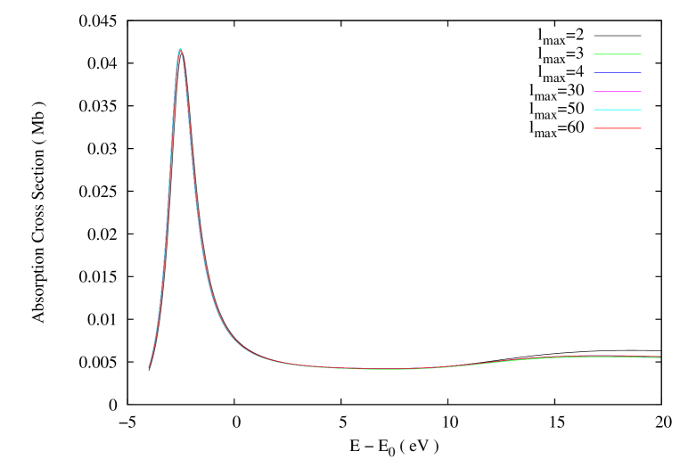
Figure 4: K-edge $z$-polarized absorption cross section for the $\sigma$ state of the $Se_{2}$ molecule, for various $l$-values up to $l_{\rm max}=60$, calculated by full inversion of the MS matrix (I-GT).

5 Applications

Application of the present FP-MS theory to two cases which, according to our experience, need significant non-MT corrections for a good reproduction of the absorption data (i.e. diatomic-linear molecules and tetrahedrally coordinated compounds) have already been presented in Ref.  [22] for the $K$-edge of $Se_{2}$ and the $Si$ $L_{2,3}$ edge of crystalline $SiO_{2}$ ($\alpha$-quartz). There it was shown that a good description of the anisotropies of the potential leads to a substantial improvement of the calculated absorption signal in comparison with the experimental spectra.

In this section we present another application to the $K$-edge absorption of $Br_{2}$ and discuss a preliminary application of the NMT approach to the study of the performance of two effective optical potentials, the Hedin-Lundqvist (HL) potential and the Dirac-Hara (DH) in the case of a transition metal.

It should be emphasized that all potentials used here and in Ref.  [22] are non-self-consistent, since the starting charge density is obtained by mere superposition of atomic densities. Therefore the agreement or disagreement with experiments might change if a self-consistent charge density were used, although from our experience the effect of this latter has a minor impact on the spectra than the elimination of the MT approximation. In any case, one of the motivations for pursuing the FP-MS method was exactly the study of the performance of the various models of optical potential together with the effect of the self-consistent charge density, once that the geometrical approximation of the potential had been eliminated. The application of the present real space theory to the generation of the self-consistent ground state density using the well known technique of contour integration in the complex energy plane is under way.

In order to obtain the absorption spectra we start from the well known expression of the absorption cross section in terms of the GF, given by

$$\sigma_{tot}(\omega) = -8\,\pi\,\alpha\,\hbar\,\omega\,$$ (119)

$$\times\sum_{m_{c}}\,\Im\int\langle\phi^{c}_{L_{c}}({\bf r})|{\hat{\varepsilon}}\cdot{\bf r}|G({\bf r},{\bf r}^{\prime};E)|{\hat{\varepsilon}}\cdot{\bf r}^{\prime}|\phi^{c}_{L_{c}}({\bf r}^{\prime})\rangle{\rm d}{\bf r}\,{\rm d}{\bf r}^{\prime}$$

For more details and other spectroscopies we refer the reader to Ref. [35]. We used all three forms of GF given by Eqs. (90), (91) and (92). While the last two are numerically stable and give almost coincident spectra, the first one shows occasionally small but noticeable kinks in the calculated spectrum and sometimes small deviations around maxima and/or minima of the cross section compared to the other two. This is a known phenomenon which is now exalted compared to the MT case, where it was almost unnoticeable. It is due the fact that the singularities of the $S$-matrix in the definition of the scattering basis functions $\overline{\Phi}({\bf r})$ in Eq. (67) and those of $T^{-1}$ in the inverted MS matrix $\tau=(T^{-1}-G)$ do not compensate exactly. Therefore, even though the three forms are formally equivalent, from a computational point of view, form Eq. (90) is to be avoided.

Fig. (5), shows the experimental unpolarized K-edge absorption cross section of the diatomic molecule $Br_{2}$ [41] in comparison with a NMT and a MT calculation as a function of the photo-electron kinetic energy $E$ referred to $E_{0}$, the true zero of the non-self-consistent molecular potential at infinity. All spectra were normalized at a common energy point between 20 and 30 eV. For the NMT case we partitioned the space with 24 Voronoi polyhedra arranged on a BCC lattice: two of them around the physical atoms and 22 empty cells (EC) to cover the rest of the space where the density (and the potential) are significantly different from zero. ${\it l}_{\rm max}$ was taken equal to 4 in all polyhedra. We gave a small finite imaginary part to the energy of the order of ($\sim$ 0.02 eV) in order to be able to use the same Green’s function expression for the cross section Eq. (119) both for bound and continuum states. To calculate the absorption spectrum, we used the real part of an Hedin-Lundqvist (HL) potential and then convoluted the result with a Lorentzian whose width is equal to the that of the core hole (2.52 eV). We see that the agreement with experiment is rather good. In contrast, the MT approximation of the potential turns out to be rather poor.

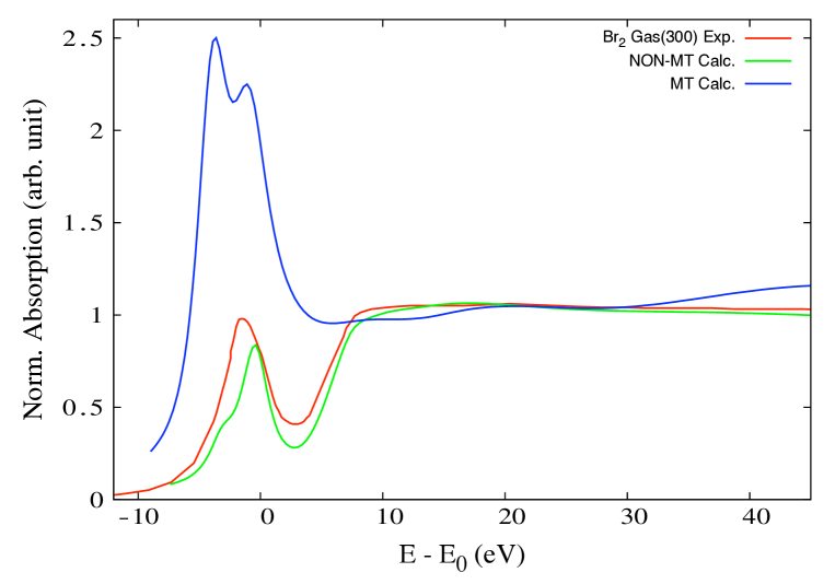
Figure 5: K-edge unpolarized absorption cross section for $Br_{2}$ molecule, showing the comparison between the MT and FP-MS calculations against the experimental data

We then present in Fig. (6) a preliminary application of the NMT approach to assess the performance of the HL against a DH potential, assuming that the losses are sufficiently well described in both cases by the imaginary part of the HL self-energy, in the case of HCP Co metal. As is well known, the real part of the HL potential is composed of two terms: the static Hartree-Fock (HF) exchange, known also as Dirac-Hara (DH) exchange, coming from the constant part of the dielectric function and the dynamically screened exchange-correlation contribution (HLXC), originating from the $\omega$-dependent part (see Appendix A of Ref.  [42]).

This calculation (and other similar along the same line) were performed without any adjustable parameter. In all cases the number of atoms forming the cluster is about 140-150, lying inside a sphere of about 7-8 Å, enough to obtain spectral convergence in the presence of the complex part of the potential. The charge density was obtained by superposition of neutral atom charge densities, from which the Coulomb and the exchange-correlation potential are calculated. In the case of close-packed structure, this fact should not be an handicap.

By contour integral of the Green’s Function over the energy range of the valence sates, the Fermi Energy was determined to be around -10 eV with respect to $E_{0}=0$, i.e. the zero of the cluster potential at infinity. It serves to define the local momentum of the photo-electron in the calculation of the HL (DH) potential, but the calculated spectra are rather insensitive to small variations of this quantity by 1-2 eV. No self-consistence loop was attempted to find a self-consistent charge. The core hole width was taken into account by adding 0.7 eV to the complex part of the potential.

Surprisingly enough, the comparison shows that the DH potential gives overall better agreement with the experiments than the HL one. A similar situation is found for other transition metals and has been reported elsewhere.  [43] Notice that the same conclusion was drawn in Ref. [44] for $Cu_{2}MnM$, where $M=Al,Sn,In$, although in the MT approximation.

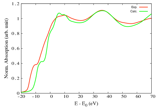
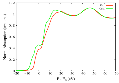
Figure 6: Comparison between Co K-edge absorption calculated with complex HL (left) and DH (right) potentials with experimental results. (Color online)

6 Conclusions

We have developed a FP-MS scheme which is a straightforward generalization of the usual theory with MT potentials and implemented the code to calculate cross sections for several spectroscopies, like absorption, photo-electron diffraction and anomalous scattering, as well as bound states, by a simple analytical continuation. The key point in this approach is the generation of the cell solutions $\Phi_{L}\,(\,{\bf r}\,)$ for a general truncated potential free of the well known convergence problems of AM expansion together with an alternative derivation of the MSE which allows us to treat the matrices $S$ and $E$ as square, with only one truncation parameter, given by the classical relation $l_{\rm max}\sim k\,R_{b}$. The fact that the theory can work with square $S$ and $E$ matrices is of the utmost importance, since this feature allows the definition of the cell $T$ matrix and its inverse, recuperating in such way the possibility to define the Green’s function and to treat a host of problems, ranging from solids with reduced symmetry to randomly disordered alloys in the context of the CPA, as mentioned in the introduction. In this way one can also show that the wave function and the Green’s function approach provide the same expression for the absorption cross section for continuum states and real potentials, through the application of the generalized optical theorem (see E). For transitions to bound states the two methods are not equivalent, due to the different normalization of continuum and bound states, unless one normalizes to one the wave function for these latter. However this procedure, although feasible, is rather cumbersome (this was one of the reasons for abandoning the MS method in favor of the simpler linearized methods in band structure calculations). Instead, the Green’s function expression for the cross section Eq. (119) can always be used, since it gives the correct normalization in both cases simply by analytical continuation. We have exploited this fact when calculating the cross section for the $Se_{2}$ and $Br_{2}$ diatomic molecules.

Moreover, in the present paper we have been able to show that the FP-MST converges absolutely in the $l_{\rm max}\rightarrow\infty$ limit (modulo a slight modification of the free propagator matrix $G$ which is practically unnecessary) in the sense that the scattering path operator of the theory can be found in terms of an absolutely convergent procedure in this limit. We have thus given a firm ground to its use as a viable method for electronic structure calculation and at the same time have provided a straightforward extension of MST in the Muffin-Tin (MT) approximation for the calculation of x-ray spectroscopies. Also Quantum Chemistry calculations might benefit from this method in that it avoids the use of basis functions sets.

Finally it is worth mentioning that in giving a new scheme to generate local basis functions for truncated potential cells, we have provided an efficient and fast method for solving numerically a partial differential equation of the elliptic type in polar coordinates, which can also be used to solve the Poisson equation in the whole space by the partitioning method.

Appendix A The Mathieu functions

For the convenience of the reader we give here a brief account of the Mathieu functions. The solution of the 3-dimensional Mathieu’s equation (22) of the text is obtained by separation of variables

$$\psi(x,y,z)=f_{x}(x)f_{y}(y)f_{z}(z).$$ (120)

in terms of functions $f$ solutions of the one-dimensional Mathieu’s equation [27]

$$\frac{d^{2}f(r)}{dr^{2}}=(-a+2q\cos 2r)f(r)$$ (121)

A solution of Eq. ( 121 ) having period $\pi$ or $2\pi$ is of the form,

$$f(r)=\sum_{m=0}^{\infty}(A_{m}\cos mr+B_{m}\sin mr)$$ (122)

where $B_{0}$ can be taken as zero. If the above expression is substituted into Eq. ( 121 ) one obtains

$$\sum_{m=-2}^{\infty}[(a-m^{2})A_{m}-q(A_{m-2}+A_{m+2})]\cos mr$$

$$+\sum_{m=-1}^{\infty}[(a-m^{2})B_{m}-q(B_{m-2}+B_{m+2})]\sin mr=0$$ (123)

with $A_{-m}=B_{-m}=0\quad{\rm if}\quad m>0$. Eq. ( 123 ) can be reduced to one of four simpler types,

$$f_{0}(r)=\sum_{m=0}^{\infty}A_{2m+p}\cos(2m+p)r,\,\,\,\,\,p=0\,\,{\rm or}\,\,1$$ (124)

$$f_{1}(r)=\sum_{m=0}^{\infty}B_{2m+p}\sin(2m+p)r,\,\,\,\,\,p=0\,\,{\rm or}\,\,1.$$ (125)

If $p=0$, the solution is of period $\pi$; if $p=1$, the solution is of period $2\pi$. $f_{0}$ is an even solution, and $f_{1}$ is an odd solution. The recurrence relations among the coefficients of these basic solutions are easily obtained from the general relations Eq. ( 123 ). For even solutions of period $\pi$ we find

$$aA_{0}-qA_{2}=0$$ (126)

$$(a-4)A_{2}-q(2A_{0}+A_{4})=0$$ (127)

$$(a-m^{2})A_{m}-q(A_{m-2}+A_{m+2})=0,\,\,\,\,\,\,\,\,m\geq 3$$ (128)

and of period $2\pi$,

$$(a-1)A_{1}-q(A_{1}+A_{3})=0$$ (129)

$$(a-m^{2})A_{m}-q(A_{m-2}+A_{m+2})=0,\,\,\,\,\,\,\,\,m\geq 3.$$ (130)

For odd solutions of period $\pi$,

$$(a-4)B_{2}-qA_{4}=0$$ (131)

$$(a-m^{2})B_{m}-q(B_{m-2}+B_{m+2})=0,\,\,\,\,\,\,\,\,m\geq 3$$ (132)

whereas for period $2\pi$,

$$(a-1)B_{1}+q(B_{1}-B_{3})=0$$ (133)

$$(a-m^{2})B_{m}-q(B_{m-2}+B_{m+2})=0,\,\,\,\,\,\,\,\,m\geq 3$$ (134)

It is convenient to separate the characteristic values $a$ into two major subsets:

$$a = a_{r},\;\;{\rm associated\,\,with\,\,even\,\,periodic\,\,solutions}$$

$$a = b_{r},\;\;{\rm associated\,\,with\,\,odd\,\,periodic\,\,solutions}$$

where $r$ describes the index of the eigenstate. Table 2 gives the first three eigenvalues associated to even periodic solutions and the first two associated to odd periodic solutions ($b_{0}=0$), for some selected values of $q$. They can serve to generate the Mathieu functions using the above recurrence relations to determine the coefficients in the solutions (124) and (125).

Table 2: First few Eigenvalues of Mathieu functions for different $q$ values

parity	even		odd
period	$\pi$	$2\pi$	$\pi$	$2\pi$
q=0.01	$a_{0}$=-4.99995$\times 10^{-6}$	$a_{1}=1.00999$	$b_{2}=3.99999$	$b_{1}=0.989988$
	$a_{2}=4.00004$
q=0.02	$a_{0}$=-1.99991$\times 10^{-5}$	$a_{1}=1.01995$	$b_{2}=3.99997$	$b_{1}=0.97995$
	$a_{2}=4.00017$
q=0.03	$a_{0}$=-4.49956$\times 10^{-5}$	$a_{1}=1.02989$	$b_{2}=3.99993$	$b_{1}=0.969888$
	$a_{2}=4.00037$
q=0.04	$a_{0}$=-7.9986$\times 10^{-4}$	$a_{1}=1.0398$	$b_{2}=3.99987$	$b_{1}=0.959801$
	$a_{2}=4.00067$
q=0.05	$a_{0}$=-1.24966$\times 10^{-3}$	$a_{1}=1.04969$	$b_{2}=3.99979$	$b_{1}=0.949689$
	$a_{2}=4.00104$
q=0.1	$a_{0}$=-4.99454$\times 10^{-3}$	$a_{1}=1.09873$	$b_{2}=3.99917$	$b_{1}=0.898766$
	$a_{2}=4.00416$
q=0.2	$a_{0}$=-1.99133$\times 10^{-2}$	$a_{1}=1.19487$	$b_{2}=3.99667$	$b_{1}=0.795124$
	$a_{2}=4.01658$
q=0.3	$a_{0}$=-4.4566$\times 10^{-2}$	$a_{1}=1.28832$	$b_{2}=3.9925$	$b_{1}=0.689166$
	$a_{2}=4.03706$
q=1	$a_{0}$=-0.455139	$a_{1}=1.85911$	$b_{2}=3.91702$	$b_{1}=-0.110249$
	$a_{2}=4.3713$
q=2	$a_{0}$=-1.51396	$a_{1}=2.3792$	$b_{2}=3.67223$	$b_{1}=-1.39068$
	$a_{2}=5.17267$
q=5	$a_{0}$=-5.80005	$a_{1}=1.85819$	$b_{2}=2.09946$	$b_{1}=-5.79008$
	$a_{2}=7.44911$
q=10	$a_{0}$=-13.937	$a_{1}=-2.39914$	$b_{2}=-2.38216$	$b_{1}=-13.9366$
	$a_{2}=7.71737$

Appendix B Asymptotic behavior of KKR Structure Factors

For $\nu\rightarrow\infty$ through real positive numbers (in practice for $\nu\gg|z|$), the other variables being fixed, one has  [27]

$$J_{\nu} \approx \bigg{(}\frac{1}{2\pi\nu}\bigg{)}^{1/2}\,\bigg{(}\frac{ez}{2\nu}\bigg{)}^{\nu};\qquad$$ (135)

$$-iH_{\nu}^{\pm}\approx\pm\bigg{(}\frac{2}{\pi\nu}\bigg{)}^{1/2}\,\bigg{(}\frac{ez}{2\nu}\bigg{)}^{-\nu}$$

where $e$ is the Neper number. Remembering that

$$j_{n}(z) = \sqrt{\frac{\pi}{2z}}\,J_{n+1/2}(z);\qquad$$ (136)

$$h^{\pm}_{n}(z)=\sqrt{\frac{\pi}{2z}}\,H_{n+1/2}^{\pm}(z)$$

we find for the asymptotic behavior of the spherical Bessel and Hankel functions

$$j_{n}(z) \approx \frac{z^{n}}{\sqrt{2}}\,e^{n+1/2}\,\bigg{(}\frac{1}{2n+1}\bigg{)}^{n+1};\qquad$$ (137)

$$-ih^{\pm}_{n}(z)\approx\frac{\sqrt{2}}{z^{n+1}}\frac{1}{e^{n+1/2}}(2n+1)^{n}$$

We need to find un upper limit for $G^{ij}_{LL^{\prime}}$ given by

$$G^{ij}_{LL^{\prime}}=-4\pi ik\sum_{L^{\prime\prime}}\,i^{l-l^{\prime}+l^{\prime\prime}}\,C(L,L^{\prime};L^{\prime\prime})\,h^{+}_{l^{\prime\prime}}(\rho)\,Y_{L^{\prime\prime}}(\hat{\rho})$$ (138)

where $\rho=kR_{ij}$, $\hat{\rho}=\hat{R_{ij}}$ and $C(L,L^{\prime};L^{\prime\prime})$ are the Gaunt coefficients. To establish an upper limit for this expression when $l$ is fixed and $l^{\prime}\gg\rho$ we replace each $|h^{+}_{l^{\prime\prime}}(\rho)|$ in the sum by its maximum value $|h^{+}_{l+l^{\prime}}(\rho)|$, use the asymptotic value in Eq. (137) and the relation $\sum_{L^{\prime\prime}}C(L,L^{\prime};L^{\prime\prime})\,Y_{L^{\prime\prime}}(\hat{\rho})=Y_{L}(\hat{\rho})Y_{L^{\prime}}(\hat{\rho})$ to obtain

$$|G^{ij}_{LL^{\prime}}| \leq 4\pi k|h^{+}_{l+l^{\prime}}(\rho)|\,\sum_{L^{\prime\prime}}|C(L,L^{\prime};L^{\prime\prime})\,Y_{L^{\prime\prime}}(\hat{\rho})|$$ (139)

$$\approx 4\pi k|h^{+}_{l+l^{\prime}}(\rho)|\,|\sum_{L^{\prime\prime}}C(L,L^{\prime};L^{\prime\prime})\,Y_{L^{\prime\prime}}(\hat{\rho})|$$

$$= 4\pi k|h^{+}_{l+l^{\prime}}(\rho)|\,|Y_{L}(\hat{\rho})Y_{L^{\prime}}(\hat{\rho})|$$

$$\leq [(2l+1)(2l^{\prime}+1)]^{1/2}\frac{\sqrt{2}}{\rho^{l+l^{\prime}+1}}\frac{k}{e^{l+l^{\prime}+1/2}}[2(l+l^{\prime})+1]^{l+l^{\prime}}$$

since $|Y_{L}(\hat{\rho})|\leq\sqrt{(2l+1)/(4\pi)}$. Notice that the approximation $\sum_{L^{\prime\prime}}|C(L,L^{\prime};L^{\prime\prime})Y_{L^{\prime\prime}}(\hat{\rho})|\approx|\sum_{L^{\prime\prime}}C(L,L^{\prime};L^{\prime\prime})\,Y_{L^{\prime\prime}}(\hat{\rho})|$ entails only errors $O(1)$ in all $l$ variables, as can be verified by explicit calculation, and therefore completely negligible with respect to the power behavior of the rest of the factors. In any case, since $\sum_{L^{\prime\prime}}|C(L,L^{\prime};L^{\prime\prime})Y_{L^{\prime\prime}}(\hat{\rho})|\leq[(2l+1)(2l^{\prime}+1)]^{1/2}/(4\pi)\sum_{L^{\prime\prime}}(2l^{\prime\prime}+1)$, at the cost of introducing a non influential extra factor $[2(l+l^{\prime})+1]^{2}$ in Eq. (139) we would get a rigorous inequality. This expression is obviously also valid for $l\gg\rho$.

Under the same conditions, assuming $l^{\prime}\gg l$ we derive

$$|J^{ij}_{LL^{\prime}}| \leq 4\pi|j_{l^{\prime}-l}(\rho)|\,|Y_{L}(\hat{\rho})Y_{L^{\prime}}(\hat{\rho})|$$ (140)

$$\leq [(2l+1)(2l^{\prime}+1)]^{1/2}\,\frac{\rho^{l^{\prime}-l}}{\sqrt{2}}\,e^{l^{\prime}-l+1/2}\,\frac{1}{[2(l^{\prime}-l)+1]^{l^{\prime}-l+1}}$$

The inequalities Eqs. (139) and (140) can be used to obtain other useful inequalities used throughout the paper. For example, for fixed $l$, using again Eq. (137), one obtains

$$|G^{ij}_{LL^{\prime}}J_{L^{\prime}}({\bf r}_{j})|\leq\left(\frac{r_{j}}{R_{ij}}\right)^{l^{\prime}}\,\frac{k}{(kR_{ij})^{l+1}}[2(l^{\prime}+l)+1]^{l}\,\sqrt{\frac{2l+1}{4\pi}}\,e^{-l}$$ (141)

implying that the series $\tilde{H}_{L}^{+}({\bf r}_{i})=\sum_{L^{\prime}}G^{ij}_{LL^{\prime}}J_{L^{\prime}}({\bf r}_{j})$ is absolutely and uniformly convergent in the angular domain. The uniform convergence comes from the application of the Weierstrass criterion (see Ref. [40], sect. 3.34, pag. 49).

Similarly one finds

$$|J^{io}_{LL^{\prime}}\tilde{H}_{L^{\prime}}^{+}({\bf r}_{o})|\leq\left(\frac{R_{io}}{r_{o}}\right)^{l^{\prime}+1}\frac{k}{(kR_{io})^{l+1}}\;[2(l^{\prime}-l)+1]^{l}\,\sqrt{\frac{2l+1}{4\pi}}\,e^{-l}$$ (142)

showing that the series $\tilde{H}_{L}^{+}({\bf r}_{i};\kappa)=\sum_{L^{\prime}}J^{io}_{LL^{\prime}}\tilde{H}_{L^{\prime}}^{+}({\bf r}_{o};\kappa)$ is also absolutely and uniformly convergent if $(r_{o}>R_{io})$.

Along the same lines we can estimate an upper bound for the atomic T-matrix for $l,\,l^{\prime}\gg kR_{b}$. We find from Eq. (39) to first order

$$T_{LL^{\prime}} = \int_{0}^{R_{b}}\,J_{L^{\prime}}({\bf r})\,V({\bf r})\,\psi_{L}({\bf r})\,{\rm d^{3}r}$$ (143)

$$= \sum_{L^{\prime\prime}L^{\prime\prime\prime}}C(L^{\prime},L^{\prime\prime};L^{\prime\prime\prime})\,\int_{0}^{R_{b}}r^{2}\,j_{l^{\prime}}(kr)\,V_{L^{\prime\prime\prime}}(r)\,R_{L^{\prime\prime}L}(r)\,{\rm dr}$$

$$\approx \sum_{L^{\prime\prime}}C(L^{\prime},L;L^{\prime\prime})\,\int_{0}^{R_{b}}r^{2}\,j_{l^{\prime}}(kr)\,V_{L^{\prime\prime}}(r)\,j_{l}(kr)\,{\rm dr}$$

where the last step follows from the fact that under the above assumptions $R_{L^{\prime}L}\approx\,j_{l}\delta_{LL^{\prime}}$. Taking into account that $C(L^{\prime},L;L^{\prime\prime})\approx 1/\sqrt{4\pi}\,O(1)$ for all L-values and using again Eq. (137) we obtain

$$|T_{LL^{\prime}}| \leq 4ll^{\prime}\,\int_{0}^{R_{b}}r^{2}\,|j_{l^{\prime}}(kr)|\,|V_{|l-l^{\prime}|}(r)|\,|j_{l}(kr)|\,{\rm dr}$$ (144)

$$\approx 4ll^{\prime}k^{l+l^{\prime}}\,\frac{e^{l+l^{\prime}+1}}{(2l+1)^{l+1}\,(2l^{\prime}+1)^{l^{\prime}+1}}$$

$$\times\int_{0}^{R_{b}}r^{l+l^{\prime}+2}\,\,|V_{|l-l^{\prime}|}(r)|\,\,{\rm dr}$$

$$\leq \frac{Z_{eff}}{k^{2}}\,\frac{4ll^{\prime}}{l+l^{\prime}+2}\,\frac{(kR_{b})^{l+l^{\prime}+2}\,e^{l+l^{\prime}+1}}{(2l+1)^{l+1}\,(2l^{\prime}+1)^{l^{\prime}+1}}$$

with the understanding that $V_{l}\equiv V_{l0}$, assuming that $|V_{l}(r)|\leq 2Z_{eff}/r$ in atomic units and that $|V_{l}(r)|$ is decreasing with $l$.

Based on the above inequalities we easily obtain

$$|G^{ij}_{LL^{\prime}}T_{LL^{\prime}}| \leq 8\sqrt{2}e^{1/2}Z_{eff}R_{b}\frac{(ll^{\prime})^{3/2}}{l+l^{\prime}+2}\,$$ (145)

$$\times\left(\frac{R_{b}}{R_{ij}}\right)^{l+l^{\prime}+1}\frac{(2l+2l^{\prime}+1)^{l+l^{\prime}}}{(2l+1)^{l+1}\,(2l^{\prime}+1)^{l^{\prime}+1}}$$

Specializing to the case where $l$ is fixed and $l^{\prime}$ is running, we also find

$$|G^{ij}_{LL^{\prime}}T_{L^{\prime}L^{\prime}}| \leq 4\frac{(ll^{\prime})^{1/2}l^{\prime}}{l^{\prime}+1}Z_{eff}\,$$ (146)

$$\times\frac{(kR_{b})^{2l^{\prime}+2}}{(kR_{ij})^{l+l^{\prime}+1}}\,\frac{e^{2l^{\prime}+1}}{e^{l+l^{\prime}+1/2}}\frac{(2l+2l^{\prime}+1)^{l+l^{\prime}}}{(2l^{\prime}+1)^{2l^{\prime}+1}}$$

which is useful in discussing questions related to the convergence of MST.

Finally we note that all the above inequalities and convergence conditions remain valid for complex arguments $\rho$, provided it is replaced by its module $|\rho|$.

Appendix C Surface identity for scattering states

In the case of short range potentials (i.e. potentials that behave like $1/r^{1+\epsilon}$ with positive $\epsilon$ as $r\rightarrow\infty$) the Lippmann-Schwinger equation for scattering states at energy $E=k^{2}$

$$\psi({\bf r};{\bf k})=\phi_{0}({\bf r};{\bf k})+\int d{\bf r}^{\prime}G_{0}({\bf r}-{\bf r}^{\prime};k)V({\bf r}^{\prime})\psi({\bf r}^{\prime};{\bf k})$$ (147)

is a consequence of the Schrödinger equation

$$(\nabla^{2}+E-V({\bf r}))\psi({\bf r};{\bf k})=0$$ (148)

together with the relations ($\phi_{0}({\bf r};{\bf k})\equiv{\rm e}^{{\rm i}{\bf k}\cdot{\bf r}}$)

$$(\nabla^{2}+E)\phi_{0}({\bf r};{\bf k})=0$$ (149)

$$(\nabla^{2}+E)G_{0}({\bf r}-{\bf r}^{\prime};k)=\delta({\bf r}-{\bf r}^{\prime})$$ (150)

Starting from Eq. (147), we derive the identity

$$\int_{\Omega}d{\bf r}^{\prime}\left[G_{0}({\bf r}-{\bf r}^{\prime};k)V({\bf r}^{\prime})-\delta({\bf r}-{\bf r}^{\prime})\right]\psi({\bf r}^{\prime};{\bf k})=-\phi_{0}({\bf r};{\bf k})$$ (151)

where $\Omega$ indicates the whole space. Using Eq. (150) to replace the delta function, and the Schrödinger equation (148) to eliminate $V({\bf r}^{\prime})$ we obtain

$$\sum_{j=1}^{N+1} \int_{\Omega_{j}}\{G_{0}({\bf r}-{\bf r}^{\prime};k)(\nabla^{2}+E)\psi({\bf r}^{\prime};{\bf k})$$

$$-\psi({\bf r}^{\prime};{\bf k})(\nabla^{2}+E)G_{0}({\bf r}-{\bf r}^{\prime};k)\}d{\bf r}_{j}^{\prime}=-\phi_{0}({\bf r};{\bf k})$$

where we have decomposed the whole space as $\Omega=\sum_{j=1}^{N+1}\Omega_{j}$, such that $\Omega_{N+1}\equiv\Omega_{o}=\mathcal{C}\sum_{j=1}^{N}\Omega_{j}$.

Transforming to surface integrals by application of the Green’s theorem

$$\sum_{j=1}^{N+1} \int_{S_{j}}\left[G_{0}({\bf r}-{\bf r}^{\prime};k)\nabla\psi({\bf r}^{\prime};{\bf k})\right.$$ (152)

$$\left.-\psi({\bf r}^{\prime};{\bf k})\nabla G_{0}({\bf r}-{\bf r}^{\prime};k)\right]\cdot{\bf n}_{j}^{\prime}d\sigma_{j}^{\prime}=-\phi_{0}({\bf r};{\bf k})$$

We now observe that the surface integral over the surface $S_{N+1}$ of the volume $\Omega_{N+1}\equiv\Omega_{o}$ has two contributions, one coming from the surface $S_{o}$ of $\sum_{j=1}^{N}\Omega_{j}$, the other one $S_{o}^{\infty}$ at infinity, as the limit as $R\rightarrow\infty$ over the surface of a sphere $S_{o}^{R}$, of radius $R$. This latter is easily calculated on the basis of the asymptotic behavior of $\psi({\bf r};{\bf k})$ in Eq. (38) and the expansion (33) and gives exactly $-\phi_{0}({\bf r};{\bf k})$, canceling the rhs term in Eq. (152). Therefore we recover the identity (29) of Section 3.1

$$\sum_{j=1}^{N}\int_{S_{j}}\{G_{0}({\bf r}-{\bf r}^{\prime},k)\nabla\psi({\bf r}^{\prime};{\bf k})$$

$${\hskip 62.59605pt}-\psi({\bf r}^{\prime};{\bf k})\nabla G_{0}({\bf r}-{\bf r}^{\prime};k)\}\cdot{\bf n}_{j}^{\prime}d\sigma_{j}^{\prime}$$

$$=\int_{S_{o}}\{G_{0}({\bf r}-{\bf r}^{\prime},k)\nabla\psi({\bf r}^{\prime};{\bf k})$$

$${\hskip 62.59605pt}-\psi({\bf r}^{\prime};{\bf k})\nabla G_{0}({\bf r}-{\bf r}^{\prime};k)\}\cdot{\bf n}_{O}^{\prime}d\sigma_{O}^{\prime}$$ (153)

Appendix D The Generalized Optical Theorem

For convenience of the reader we give here a proof of Eq. (76) in the case where $\overline{T}^{o}\equiv 0$, i.e. when empty cells cover the volume $\Omega_{o}$ up to the point at which the asymptotic behavior in Eq. (38) begins to be valid. We start by observing that

$$\int{d\hat{\bf k}}\,I_{L^{\prime}}^{i}({\bf k})\,\left[I_{L}^{j}({\bf k})\right]^{\ast}=J_{LL^{\prime}}^{ij}\,\frac{k}{\pi}$$ (154)

so that, using the relation Eq. (74), we find

$$\int{\rm d}\hat{\bf k}\,B^{i}_{L^{\prime}}({\bf k})\,\left[B^{j}_{L}({\bf k})\right]^{\ast}=\sum_{L\Lambda}\,\tau_{L\Lambda^{\prime}}^{im}\,J_{\Lambda\Lambda^{\prime}}^{mn}\,(\tau_{\Lambda^{\prime}L^{\prime}}^{ni})^{\ast}\,\frac{k}{\pi}$$ (155)

where we have used the symmetry of $\tau$. Based on the relations Eqs. (99), (100) and (102), valid at any energy, and due to the reality of the matrices $K$, $N$ and $J$ for real potential, we can write

$$\tau=k^{-1}\,\left[K-N+iJ\right]^{-1}$$ (156)

so that the rhs of Eq. (155) becomes

$$\frac{k}{\pi}\,\left\{\tau\,J\,\tau\right\}_{LL^{\prime}}^{ij}=\frac{1}{\pi}\,\frac{1}{2i}\left\{\tau^{\ast}-\tau\right\}_{LL^{\prime}}^{ij}=-\frac{1}{\pi}\,\Im\tau_{LL^{\prime}}^{ij}$$ (157)

in keeping with Eq. (76).

Appendix E Wave function and GF equivalence for absorption cross section

In the independent electron approximation, the core level photoelectron diffraction (PED) cross-section for the ejection of a photoelectron along the direction $\hat{\bf k}$ and energy $E=k^{2}$ from an atom situated at site $i$ is given by [35]

$$\frac{d\sigma}{d\hat{\bf k}}=8\,\pi^{2}\,\alpha\,\hbar\,\omega\,\sum_{m_{c}}\left|\langle\Theta\psi({\bf r}_{i};{\bf k})|{\hat{\varepsilon}}\cdot{\bf r}_{i}|\phi^{c}_{L_{c}}({\bf r}_{i})\rangle\right|^{2}$$ (158)

Here $\Theta$ is the time-reversal operator, $\hat{\varepsilon}$ the polarization of the incident photon and $\phi^{c}_{L_{c}}({\bf r}_{i})$ the initial core state of angular momentum $L_{c}$ (we neglect for simplicity the spin-orbit coupling, which can be easily taken into account). Due to the localization of the core state, we need only the expression of the continuum scattering state in the cell of the photoabsorber, given by

$$\psi({\bf r}_{i};{\bf k})=\sum_{L}B^{i}_{L}({\bf k})\overline{\Phi}_{L}({\bf r}_{i})$$ (159)

so that

$$\frac{d\sigma}{d\hat{\bf k}}=8\,\pi^{2}\,\alpha\,\hbar\,\omega\,\sum_{m_{c}}\left|\sum_{L}M_{L_{c}L}(E)\,B^{i}_{L}({\bf k})\right|^{2}$$ (160)

where $B^{i}_{L}({\bf k})$ is given by Eq. (74) and we have defined the atomic transition matrix element

$$M_{L_{c}\,L}\,(E)\,=\,\int_{{\Omega}_{i}}d\,{\bf r}\,\phi^{c}_{L_{c}}({\bf r})\,{\hat{\varepsilon}}\cdot{\bf r}\,\overline{\Phi}_{L}({\bf r})$$ (161)

The total absorption cross-section, in the case of real potentials, is obtained by integrating the PED cross-section over all directions of photoemission

$$\int{d\hat{\bf k}}\,\frac{d\sigma}{d\hat{\bf k}} = 8\,\pi^{2}\,\alpha\,\hbar\,\omega\,\sum_{m_{c}}\int{d\hat{\bf k}}\,\left|\sum_{L}M_{L_{c}L}(E)\,B^{i}_{L}({\bf k})\right|^{2}$$ (162)

$$= -8\,\pi\,\alpha\,\hbar\,\omega\,\sum_{m_{c}}\sum_{LL^{\prime}}\,M_{L_{c}\,L}\,(E)\Im\tau_{LL^{\prime}}^{ii}M_{L_{c}\,L^{\prime}}$$

by application of the optical theorem (76). This is exactly the form that one would obtain starting from Eq. (119) and using the expression (90) for the GF.

Appendix F Exploitation of point symmetry

In a cluster (to which we shall also refer as a molecule), point symmetry can be used to advantage to simplify the problem and reduce the size of the MS matrix. Specifically we consider the case where the cluster remains invariant under a finite group of transformations $\mathcal{G}$ relative to the molecular center $R_{o}$. This group has a finite number of finite-dimensional irreducible representations (irreps) $\Gamma_{j}$ ($j=1,2,...,g$). Due to the symmetry, the cluster will consist of $\mathcal{P}$ groups of equivalent atoms, transforming into one another under the operations of the group; and for each group $p=1,2,....,\mathcal{P}$, there are $N_{p}$ atoms labeled by $i_{p}$. If $N$ is the total number of atoms in the cluster, then $N=\sum_{p=1}^{\mathcal{P}}N_{p}$.

Under these assumptions there exists a unitary transformation $\mathcal{C}$ that block-diagonalizes the MS matrix according to the irreps. For each value of the angular momentum index $l$, this transformation is labeled by the angular projection $m$ and the site $i_{p}$ on one side, and on the other the irrep, the row $\rho$ of the irrep and a further index $n$ that distinguishes independent orthogonal symmetrized basis functions with the same $l$. The matrix elements of $\mathcal{C}$ are easily obtained by applying the projection operator $\sum_{R}M_{\rho\rho}^{\Gamma_{j}}(R)\,P_{R}$ to a spherical harmonic function $Y_{lm}(\,\hat{\bf r}_{i_{p}})\,\theta(R_{b}-r_{i_{p}})$ centered on the site $i_{p}$ and defined on the surface of the bounding sphere $R_{b}$ of the cell $\Omega_{i_{p}}$ Here $P_{R}$ is the generic operation belonging to the group $\mathcal{G}$ corresponding to the coordinate transformation $R$, and $M_{\rho\rho}^{\Gamma_{j}}(R)$ is the matrix element corresponding to $R$ in the matrix representation of irrep $\Gamma_{j}$ of the group, $\rho$ labeling the row of the irrep. As usual in group theory [45] the effect of $P_{R}$ on the function $f({\bf r})$ is given by $f(R^{-1}\,{\bf r})$. In this way, if the result is not zero, one generates a symmetrized spherical harmonic function given by

$$K_{ln}^{\Gamma_{j}^{\rho},\,p}(\,\hat{\bf r}_{p}\,) \equiv \sum_{R}M_{\rho\rho}^{\Gamma_{j}}(R)\,P_{R}\,Y_{lm}(\,\hat{\bf r}_{i_{p}})$$ (163)

$$= \sum_{R}\,M_{\rho\rho}^{\Gamma_{j}}(R)\,\sum_{\mu}D^{l}_{\mu m}(R)\,Y_{l\mu}(\,\hat{\bf r}_{i_{p}^{\prime}})$$

$$= \sum_{m,i_{p}}C_{ln,\,m}^{\Gamma_{j}^{\rho},\,{i_{p}}}\,Y_{lm}(\,\hat{\bf r}_{i_{p}}\,)$$

where $D^{l}_{\mu m}(R)$ is the Wigner rotation matrix corresponding to the transformation $R$ [45] and $i_{p}^{\prime}=R\,i_{p}$. Due to the orthogonality of the basis functions

$$\int\,Y_{lm}(\,\hat{\bf r}_{i_{p}})\,Y_{lm^{\prime}}(\,\hat{\bf r}_{i_{p}^{\prime}})\,{\rm d}\Omega = \delta_{mm^{\prime}}\,\delta_{i_{p}i_{p}^{\prime}}$$

$$\int\,K_{ln}^{\Gamma_{j}^{\rho},\,p}(\,\hat{\bf r}_{p}\,)K_{l^{\prime}n^{\prime}}^{\Gamma_{j^{\prime}}^{\rho^{\prime}},\,p}(\,\hat{\bf r}_{p}\,)\,{\rm d}\Omega = \delta_{ll^{\prime}}\,\delta_{nn^{\prime}}\,\delta_{\Gamma_{j}\Gamma_{j^{\prime}}}\,\delta_{\rho\rho^{\prime}}$$ (164)

we obtain ${\mathcal{C}}\,\tilde{\mathcal{C}}=\tilde{\mathcal{C}}\,{\mathcal{C}}=I$, i.e.

$$\sum_{m,\,i_{p}}C_{ln,\,m}^{\Gamma^{\rho},\,{i_{p}}}\,C_{l^{\prime}n^{\prime},\,m}^{\Gamma^{\prime\rho^{\prime}},\,{i_{p}}} = \delta_{ll^{\prime}}\,\delta_{nn^{\prime}}\,\delta_{\Gamma\Gamma^{\prime}}\,\delta_{\rho\rho^{\prime}}$$

$$\sum_{\Gamma\rho}\sum_{n}C_{ln,\,m}^{\Gamma^{\rho},\,i_{p}}\,C_{ln,\,m^{\prime}}^{\Gamma^{\rho},\,i_{p}^{\prime}} = \delta_{mm^{\prime}}\,\delta_{i_{p}i_{p}^{\prime}}$$ (165)

where for simplicity we have dropped the index $j$ from the symbol $\Gamma$ of the irreps.

Now, if $M\equiv M_{LL^{\prime}}^{ij}\equiv(T^{-1}-G)_{LL^{\prime}}^{ij}$ is the MS matrix in the non-symmetrized site and angular momentum indices, its symmetrized version is given by $M_{s}={\mathcal{C}}\,M\tilde{\mathcal{C}}$. Therefore for any representation $\Gamma$ we have, putting for short $\Lambda=(l,\,n)$ and remembering that $L\equiv(l,m)$,

$$T^{\Gamma,\,p}_{\Lambda,\,\Lambda^{\prime}} = \sum_{i_{p}}^{N_{p}}\sum_{m,\,m^{\prime}}\,C_{\Lambda,\,L}^{\Gamma,\,{i_{p}}}\,T^{i_{p}}_{L,\,L^{\prime}}\,C_{\Lambda^{\prime},\,L^{\prime}}^{\Gamma,\,{i_{p}}}$$ (166)

$$G^{\Gamma,\,p\,q}_{\Lambda,\,\Lambda^{\prime}} = \sum_{i_{p}}^{N_{p}}\sum_{i_{q}}^{N_{q}}\sum_{m,\,m^{\prime}}\,C_{\Lambda,\,L}^{\Gamma,\,{i_{p}}}\,G^{i_{p}\,i_{q}}_{L,\,L^{\prime}}\,C_{\Lambda^{\prime},\,L^{\prime}}^{\Gamma,\,{i_{q}}}$$ (167)

Here $T^{\Gamma,\,p}_{s}$ describes total scattering power of group $p$ and $G^{\Gamma,\,p\,q}_{s}$ is the symmetrized matrix of the KKR structure factors. The presence of an outer sphere contribution $J\overline{T}^{o}J$ is treated on the same footing and contributes ${\mathcal{C}}\,J\overline{T}^{o}J\,\tilde{\mathcal{C}}\equiv{\mathcal{C}}\,J\tilde{\mathcal{C}}\,{\mathcal{C}}\,\overline{T}^{o}\,\tilde{\mathcal{C}}\,{\mathcal{C}}\,J\,\tilde{\mathcal{C}}\equiv J_{s}\,\overline{T}^{o}_{s}\,J_{s}$ for each representation $\Gamma$. Since the outer sphere is centered at the origin of the cluster, it has no partner spheres equivalent to itself.

All these matrices are labeled only by the groups of equivalent atoms (prototypical atoms), the angular momentum $l$ and possibly the index $n$ mentioned above, realizing a sizable reduction in dimensions. Notice that, since the molecular hamiltonian is invariant under the operations of $\mathcal{G}$, the symmetrized matrix elements do not depend on the row $\rho$ of the representation $\Gamma$. Moreover, in order to find the symmetrized $T$-matrix relative to an equivalent group of atoms, we do not need to calculate $T_{LL^{\prime}}^{i_{p}}$ for all sites in the group, since these are related to one another by the relation

$$T_{LL^{\prime}}^{i_{p}^{\prime}}=\sum_{\mu\mu^{\prime}}\,D^{l}_{m\mu}(R)\,T_{l\mu\,l^{\prime}\mu^{\prime}}^{i_{p}}D^{l^{\prime}}_{m^{\prime}\mu^{\prime}}(R)$$ (168)

where, as before, $i_{p}^{\prime}=R\,i_{p}$. This relation is a consequence of the invariance of the potential and the $T$-matrix $T^{i_{p}}(\hat{\bf r},\hat{\bf r}^{\prime})$ under the operations of the group $\mathcal{G}$. Specifically

$$V_{LL^{\prime}}^{i_{p}} = \int Y_{L}(\hat{\bf r})\,V^{i_{p}}(r,\hat{\bf r})\,Y_{L^{\prime}}(\hat{\bf r})\,{\rm d}\,\hat{\bf r}$$

$$= \int Y_{L}(\hat{\bf r})\,V^{i_{p}^{\prime}}(r,R\,\hat{\bf r})\,Y_{L^{\prime}}(\hat{\bf r})\,{\rm d}\,\hat{\bf r}$$

$$= \int Y_{L}(R^{-1}\hat{\bf r})\,V^{i_{p}^{\prime}}(r,\hat{\bf r})\,Y_{L^{\prime}}(R^{-1}\hat{\bf r})\,{\rm d}\,\hat{\bf r}$$

$$= D^{l}_{\mu m}(R)\,V_{l\mu\,l^{\prime}\mu^{\prime}}^{i_{p}^{\prime}}\,D^{l^{\prime}}_{\mu^{\prime}m^{\prime}}(R)$$

valid also for the matrix elements $T_{LL^{\prime}}^{i_{p}}=\int Y_{L}(\hat{\bf r})\,T^{i_{p}}(\hat{\bf r},\hat{\bf r}^{\prime})\,Y_{L^{\prime}}(\hat{\bf r}^{\prime})\,{\rm d}\,\hat{\bf r}\,{\rm d}\,\hat{\bf r}^{\prime}$. Notice that the transformation and symmetrization properties are the same for $T$ and $T^{-1}$, so we can act directly on this latter.

In the MT case the $T$-matrices are angular momentum diagonal and $m$ and site independent within a set of equivalent atoms, so that

$$T^{\Gamma,\,p}_{\Lambda,\,\Lambda^{\prime}} = T^{p}_{l}\,\sum_{i_{p}}^{N_{p}}\sum_{m}\,C_{\Lambda,\,L}^{\Gamma,\,{i_{p}}}\,C_{\Lambda^{\prime},\,L}^{\Gamma,\,{i_{p}}}$$ (169)

$$= T^{p}_{l}\,\delta_{\Lambda,\,\Lambda^{\prime}}\,$$

The group $T^{p}$-matrix can also be calculated directly from the symmetrization of the radial part of the basis function $R_{LL^{\prime}}(r_{i_{p}})$, which transforms as $T$ in Eqs. (166) and (168). Even though the number and type of operations to perform are exactly the same as for obtaining $T^{p}$, in this case there is the added advantage of generating a symmetrized form of the scattering wave function, needed for example to calculate the absorption or photo-emission cross-section.

The symmetrization of the local wave function in a group of equivalent atoms for an irrep $\Gamma$ is obtained by observing that the following function $\psi({\bf r}_{p})$ is invariant under any operation of the group

$$\psi({\bf r}_{p}) = \,\sum_{i_{p}}\sum_{LL^{\prime}}\,A_{L}^{i_{p}}\,R_{L^{\prime}L}^{i_{p}}(r_{i_{p}})\,Y_{L^{\prime}}(\,\hat{\bf r}_{i_{p}}\,)$$ (170)

$$\equiv \langle A|R|Y\rangle$$

$$= \langle A|\tilde{\mathcal{C}}{\mathcal{C}}R\tilde{\mathcal{C}}{\mathcal{C}}|Y\rangle$$

$$= \sum_{\Lambda\Lambda^{\prime}}A_{\Lambda}^{\Gamma,\,p}\,R_{\Lambda^{\prime}\Lambda}^{\Gamma,\,p}(r_{p})\,K_{\Lambda^{\prime}}^{\Gamma,\,p}(\,\hat{\bf r}_{p}\,)$$

whereby

$$A_{\Lambda}^{\Gamma,\,p} = \sum_{m\,i_{p}}C_{\Lambda,m}^{\Gamma,\,i_{p}}\,A_{lm}^{i_{p}}$$

$$R_{\Lambda\Lambda^{\prime}}^{\Gamma,\,p}(r_{p}) = \sum_{i_{p}}^{N_{p}}\sum_{m,\,m^{\prime}}\,C_{\Lambda,\,L}^{\Gamma,\,{i_{p}}}\,R^{i_{p}}_{L,\,L^{\prime}}\,(r_{p})\,C_{\Lambda^{\prime},\,L^{\prime}}^{\Gamma,\,{i_{p}}}$$

Inside the MT sphere $X_{\Lambda^{\prime}\Lambda}^{\Gamma,\,p}(r_{p})\equiv r\,R_{\Lambda^{\prime}\Lambda}^{\Gamma,\,p}(r_{p})$ is solution of the symmetrized equation (12)

$$\sum_{\Lambda^{\prime\prime}}\left[\left(\frac{d^{2}}{dr^{2}}+E-\frac{l(l+1)}{r^{2}}\right)\delta_{\Lambda\Lambda^{\prime\prime}}-V_{\Lambda\Lambda^{\prime\prime}}^{p}(r)\right]X_{\Lambda^{\prime\prime}\Lambda^{\prime}}^{\Gamma,\,p}(r)=0$$ (171)

where we have written for simplicity $r$ for $r_{p}$ and $V_{\Lambda\Lambda^{\prime\prime}}^{p}(r)$ is given by

$${V}^{\Gamma_{1},\,p}_{\Lambda,\,\Lambda^{\prime}}(r)=\sum_{i_{p}}^{N_{p}}\sum_{m,\,m^{\prime}}\,C_{\Lambda,\,L}^{\Gamma_{1},\,{i_{p}}}\,V^{i_{p}}_{L,\,L^{\prime}}(r)\,C_{\Lambda^{\prime},\,L^{\prime}}^{\Gamma_{1},\,{i_{p}}}$$ (172)

$\Gamma_{1}$ being the identical representation of the group $\mathcal{G}$. Near the origin $X_{\Lambda\Lambda^{\prime}}^{\Gamma,\,p},(r)\sim r\,j_{l}(kr)\,K_{\Lambda}^{\Gamma,\,p}(\,\hat{\bf r}_{p}\,)\,\delta_{\Lambda\Lambda^{\prime}}$.

Across the truncated boundary, we instead use the symmetrized version of Eq. (1), so that putting $P_{\Lambda}^{\Gamma,\,p}({\bf r}_{p})=r\Phi_{\Lambda}^{\Gamma,\,p}({\bf r}_{p})$ and dropping again the index $p$

$$\left[\frac{d^{2}}{dr^{2}}+E-V(r,\hat{\bf r})\right]\,P_{\Lambda}^{\Gamma}(r,\hat{\bf r})=\frac{1}{r^{2}}\,\tilde{L}^{2}\,P_{\Lambda}^{\Gamma}(r,\hat{\bf r})$$ (173)

where

$$\tilde{L}^{2}P_{\Lambda}^{\Gamma}(r,\hat{\bf r})=\sum_{\Lambda^{\prime}}l^{\prime}(l^{\prime}+1)rR_{\Lambda^{\prime}\Lambda}^{\Gamma}(r)K_{\Lambda^{\prime}}^{\Gamma}(\,\hat{\bf r}\,)$$ (174)

and we use starting values given by Eq. (171). Equation (173) is obtained from Eq. (1) by applying on the left the projection operator $\sum_{R}M_{\rho\rho}^{\Gamma_{j}}(R)\,P_{R}$, taking into account that $V({\bf r}_{i_{p}})=V(R^{-1}\,{\bf r}_{i_{p}^{\prime}})$.

In terms of $R_{\Lambda\Lambda^{\prime}}^{\Gamma}(r)$ is then possible to define the symmetrized version of the matrices $E_{LL^{\prime}}^{i_{p}}$ and $S_{LL^{\prime}}^{i_{p}}$ as

$$E_{\Lambda\Lambda^{\prime}}^{p} = ({R_{b}^{p}})^{2}W[-i\kappa h_{l}^{+},R_{\Lambda\Lambda^{\prime}}^{p}]$$ (175)

$$S_{\Lambda\Lambda^{\prime}}^{p} = ({R_{b}^{p}})^{2}W[j_{l},R_{\Lambda\Lambda^{\prime}}^{p}]$$ (176)

and derive the symmetrized equivalent of all the quantities introduced toward the end of section (3.1). In particular the amplitudes $B^{p}_{\Lambda}({\bf k})$ are solutions of the symmetrized MSE

$$\sum_{q\,\Lambda^{\prime}}\left[{(T^{-1})}^{\Gamma,\,p}_{\Lambda,\,\Lambda^{\prime}}\,\delta_{pq}+G^{\Gamma,\,p\,q}_{\Lambda,\,\Lambda^{\prime}}\right]\,B^{q}_{\Lambda^{\prime}}({\bf k})=I^{p}_{\Lambda}({\bf k})$$ (177)

where $I^{p}_{\Lambda}({\bf k})=\sum_{m\,i_{p}}C_{\Lambda,m}^{\Gamma,\,i_{p}}\,I_{lm}^{i_{p}}({\bf k})$. Assuming that the photo-absorber is located in cell $\Omega_{o}$ at the origin of the coordinates $R_{o}$, the symmetrized PED cross section for the final state irrep $\Gamma$ with degeneracy $d(\Gamma)$ takes the form

$$\frac{d\sigma^{\Gamma}}{d\hat{\bf k}}=8\,\pi^{2}\,\alpha\,\hbar\,\omega\,d(\Gamma)\sum_{n_{c}}\left|\sum M_{\Lambda_{c}\Lambda}^{\Gamma_{c}\Gamma}(E)\,B^{o}_{\Lambda}({\bf k})\right|^{2}$$ (178)

where the atomic dipole transition matrix element

$$M_{\Lambda_{c}\,\Lambda}^{\Gamma_{c}\Gamma}\,(E)\,=\,\int_{{\Omega}_{o}}\,\phi^{\Gamma_{c}}_{\Lambda_{c}}({\bf r})\,D^{\Gamma_{d}}({\bf r})\,\overline{\Phi}_{\Lambda}^{\Gamma}({\bf r})\,{\rm d}\,{\bf r}$$ (179)

obeys the selection rules of the Wigner-Eckart theorem [45] for the finite group $\mathcal{G}$. We have assumed that the dipole operator transforms according to the irrep $\Gamma_{d}$.

Appendix G Finiteness of $Tr\,(K_{s}^{\dagger}K_{s})$

In this appendix we show that $Tr\,(K_{s}^{\dagger}K_{s})$ is finite. Starting from Eq. (111), we partition the space and the potential in the way described at the beginning of Section 3.1 and define a new kernel $\tilde{K}$ that coincides with the kernel ${\bf K}_{s}$ for ${\bf r}$ and ${\bf r}^{\prime}$ in different cells and vanishes identically when ${\bf r}$ and ${\bf r}^{\prime}$ happen to be in the same cell.

For this new kernel, $Tr(\tilde{K}^{\dagger}\tilde{K})$ is finite ($\leq N<\infty$) for an even larger class of potentials than that defined by Eq. (111) so that, rewriting ${\tilde{K}}({\bf r},{\bf r}^{\prime})$ in operator notation, we have

$$N \geq \,\int{\rm d}{\bf r}\,\left<{\bf r}|{\tilde{K}}^{\dagger}{\tilde{K}}|{\bf r}\right>$$ (180)

$$= \,\int\int\int{\rm d}E{\rm d}E^{\prime}{\rm d}E^{\prime\prime}\,\sum_{LL^{\prime}L^{\prime\prime}}\,\int{\rm d}{\bf r}\,\left<{\bf r}|J_{L}(E)\right>\,$$

$$\times\left<J_{L}(E)|{\tilde{K}}^{\dagger}|J_{L^{\prime}}(E^{\prime})\right>\left<J_{L^{\prime}}(E^{\prime})|{\tilde{K}}|J_{L^{\prime\prime}}(E^{\prime\prime})\right>\left<J_{L^{\prime\prime}}(E^{\prime\prime})|{\bf r}\right>$$

$$= \int\int{\rm d}E{\rm d}E^{\prime}\,\sum_{LL^{\prime}}|{\tilde{K}}_{LL^{\prime}}(E,E^{\prime})|^{2}$$

$$\geq \sum_{LL^{\prime}}|{\tilde{K}}_{LL^{\prime}}(E,E)|^{2}$$

taking into account that the functions $J_{L}(E)({\bf r})=(k/\pi)^{1/2}j_{l}(kr)Y_{L}(\hat{\bf r})$, with the normalization to one state per Rydberg, form a complete orthonormal set.

Now it is easy to see that the matrix ${\tilde{K}}_{LL^{\prime}}$ is the asymptotic form of the kernel $K_{s}$ in Eq. (115) for high values of the indices $LL^{\prime}$, since

$${\tilde{K}}_{LL^{\prime}}(E,E)$$

$$=\sum_{i\neq j}\int_{\Omega_{i}}{\rm d}{\bf r}_{i}\,J_{L}(E)({\bf r}_{i})|V_{i}({\bf r}_{i})|^{1/2}v_{i}({\bf r}_{i})\,$$

$$\times\int_{\Omega_{j}}{\rm d}{\bf r}_{j}^{\prime}G_{0}^{+}({\bf r}_{i}-{\bf r}_{j}^{\prime}+{\bf R}_{ij};{k})|V_{j}({\bf r}_{j}^{\prime})|^{1/2}v_{j}({\bf r}_{j}^{\prime})J_{L}(E)({\bf r}_{j}^{\prime})$$

$$=\sum_{i\neq j}\sum_{\Lambda\Lambda^{\prime}}\int_{\Omega_{i}}{\rm d}{\bf r}_{i}\,J_{L}(E)({\bf r}_{i})|V_{i}({\bf r}_{i})|^{1/2}v_{i}({\bf r}_{i})J_{\Lambda}(E)({\bf r}_{i})\;\tilde{G}^{ij}_{\Lambda\Lambda^{\prime}}\,$$

$$\times\int_{\Omega_{j}}{\rm d}{\bf r}_{j}\,J_{\Lambda}(E)({\bf r}_{j}^{\prime})\,|V_{j}({\bf r}_{j}^{\prime})|^{1/2}v_{j}({\bf r}_{j}^{\prime})J_{L}(E)({\bf r}_{j}^{\prime})$$

$$\sim\sum_{i\neq j}\sum_{\Lambda\Lambda^{\prime}}\left[T^{i}_{L\Lambda}\right]^{1/2}\,\tilde{G}^{ij}_{\Lambda\Lambda^{\prime}}\,\left[T^{i}_{\Lambda^{\prime}L^{\prime}}\right]^{1/2}$$ (181)

the last line following by the fact that asymptotically, when $L\Lambda,L^{\prime}\Lambda^{\prime}\gg kR_{b}^{i}\;(\forall i)$,

$$\left[T^{i}_{L\Lambda}\right]^{1/2}\sim\int_{\Omega_{i}}{\rm d}{\bf r}_{i}\,J_{L}(E)({\bf r}_{i})|V_{i}({\bf r}_{i})|^{1/2}v_{i}({\bf r}_{i})J_{\Lambda}(E)({\bf r}_{i})$$ (182)

Notice also that we have used the two center expansion for the free Green’s Function

$$G_{0}^{+}({\bf r}-{\bf r}^{\prime};{k})=J_{\Lambda}(E)({\bf r}_{i})\,\tilde{G}^{ij}_{\Lambda\Lambda^{\prime}}\,J_{\Lambda}(E)({\bf r}_{j}^{\prime})$$ (183)

which might diverge if $r_{i}+r_{j}>R_{ij}$, e. g. for neighboring cells. A similar problem is encountered when formulating the variational derivation of MST (see, for example, section 6.5.3, page 140 and following of Ref. [13]). One way to solve it is to use the displaced cell approach [13], whereby one can write

$${\tilde{K}}_{LL^{\prime}}(E,E)$$

$$=\sum_{i\neq j}\sum_{\underline{\Lambda}}\left\{\sum_{\Lambda\Lambda^{\prime}}\left[T^{i}_{L\Lambda}\right]^{1/2}\,J_{\Lambda\underline{\Lambda}}({\bf b}){G}_{\underline{\Lambda}\Lambda^{\prime}}({\bf R}_{ij}+{\bf b})\,\left[T^{i}_{\Lambda^{\prime}L^{\prime}}\right]^{1/2}\right\}$$ (184)

provided that $|{\bf R}_{ij}+{\bf b}|>R_{b}^{i}+R_{b}^{j}$ and the sums inside the curly brakets be performed first. Here $J_{\Lambda\underline{\Lambda}}({\bf b})$ is the usual translation operator in MST, given by Eq. (48) with the vector ${\bf R}_{ij}$ replaced by the vector ${\bf b}$. The tilde over the symbol ${G}^{ij}_{\Lambda\Lambda^{\prime}}$ in Eq. (183) was meant to be a reminder to use this procedure. Notice that the vector ${\bf b}$ depends only on the geometry of the partition of the space in cells and is independent on $l$.

In this way the expression Eq. (184) is always convergent and is such that $\sum_{LL^{\prime}}|{\tilde{K}}_{LL^{\prime}}(E,E)|^{2}=Tr({\tilde{K}}^{\dagger}{\tilde{K}})$ is finite. Consequently also $Tr\,(K_{s}^{\dagger}K_{s})$ is finite.

References

References

• [1] Korringa J 1947 Physica 13 392–400
• [2] Kohn W and Rostoker N 1954 Phys. Rev. 94 1111–1120
• [3] Slater J C and Johnson K H 1972 Phys. Rev. B 5 844–853
• [4] Andersen O 1975 Phys. Rev. B 12 3060–3083
• [5] Koelling D and Arbman G 1975 J. Phys. F 5 2041
• [6] Bei der Kellen S and Freeman A J 1996 Phys. Rev. B 54 11187–11198
• [7] Huhne T, Zecha C, Ebert H, Dederichs P and Zeller R 1998 Phys. Rev. B 58 10236–10246
• [8] Asato M, Settels A, Hoshino T, Asada T, Blügel S, Zeller R and Dederichs P 1999 Phys. Rev. B 60 5202–5210
• [9] Papanikolau N, Zeller R and Dederichs P 2002 J. Phys.: Condens. Matter 14 2799–2823
• [10] Ogura M and Akai H 2005 J. Phys.: Condens. Matter 17 5741–5755
• [11] Nesbet R K 1992 Phys. Rev. B 45 11491–11495
• [12] Butler W H, Gonis A and Zhang X G 1992 Phys. Rev. B 45 11527–11541
• [13] Gonis A and Butler W H 2000 Multiple Scattering in Solids (New York: Springer Verlag, Inc.) and references therein
• [14] Huhne T and Ebert H 1999 Solid State Commun. 109 577–582
• [15] Ankudinov A L and Rehr J J 2005 Phys. Scr. T115 24–27
• [16] Natoli C R, Benfatto M, Brouder C, RuizLópez M F and Foulis D L 1990 Phys. Rev. B 42 1944–1968
• [17] Foulis D L, Pettifer R F, Natoli C R and Benfatto M 1990 Phys. Rev. A 41 6922–6927
• [18] Foulis D L Exact distorted-wave approach to multiple-scattering theory for general potentials to be published
• [19] Joly Y 2001 Phys. Rev. B 63 125120:1–10
• [20] Taillefumier M, Cabaret D, Flank A and Mauri F 2002 Phys. Rev. B 66 195107
• [21] Hatada K, Hayakawa K, Benfatto M and Natoli C R 2007 Phys. Rev. B 76 060102R1–4
• [22] Hatada K, Hayakawa K, Benfatto M and Natoli C R 2009 J. Phys.: Condens. Matter 21 104206 (12pp)
• [23] Williams A R and van W Morgan J 1974 J. Phys. C: Solid State Phys. 7 37–60
• [24] Kellog O D 1954 Foundations of Potential Theory (New York: Dover) pag. 259
• [25] Lebedev V I 1975 Computational Mathematics and Mathematical Physics 15 44–51
• [26] Wang X G and Jr T C 2003 Journal of Theoretical and Computational Chemistry 4 599–608
• [27] Abramowitz M and Stegun I N (eds) 1972 Handobook of Mathematical Functions With Formulas, Graphs, and Mathematical Tables (Washington, D. C.: U. S. Goverment Printing Office)
• [28] Becke A D 1988 J. Chem. Phys. 88 2547–2553
• [29] Brastev V F 1966 Atomic Wavefunctions (Moscow: Nauka)
• [30] Fischer C F 1977 The Hartree-Fock Method for Atoms (John Wiley & Sons)
• [31] Mitchell A R and Griffiths D F 1977 The finite difference method in partial differential equations (John Wiley & Sons)
• [32] Amusia M Y and Chernysheva L V 1997 Computation of Atomic Processes (London: IOP publishing)
• [33] Natoli C R, Benfatto M and Doniach S 1986 Phys. Rev. A 34 4692–4694
• [34] Foulis D L 1988 The Effect of the Use of Full Potentials in the Calculation of X-Ray Absorption Near-Edge Structure by Multiple-Scattered-Wawe X-alpha Method Ph.D. thesis University of Warwick
• [35] Sebilleau D, Gunnella R, Wu Z Y, Matteo S D and Natoli C R 2006 J. Phys.: Cond. Matter 18 R175–R230
• [36] Faulkner J S and Stocks G M 1980 Phys. Rev. B 21 3222–3242
• [37] Smith F C and Johnson K H 1969 Phys. Rev. Lett. 22 1168–1171
• [38] Benfatto M, Natoli C R, Bianconi A, Garcia J, Marcelli A, Fanfoni M and Davoli I 1986 Phys. Rev. B 34 5774–5781
• [39] Tricomi F G 1985 Integral Equations (New York: Courier Dover Publications)
• [40] Whittaker E and Watson G 1965 A course of modern analysis (Cambridge: Cambridge University Press)
• [41] Filipponi A, Ottaviano L, Passacantando M, Picozzi P and Santucci S 1993 Phys. Rev. E 48 4575–4583
• [42] Natoli C R, Benfatto M, Longa S D and Hatada K 2003 J. Synchrotron Rad. 10 26–42
• [43] Hatada K, Hayakawa K, Chaboy J and Natoli C R 2009 J. Phys.: Conference Series 190 012010 (4pp)
• [44] Hatada K and Chaboy J 2007 Phys. Rev. B 76 104411:1–6
• [45] Tinkham M 1964 Group Theory and Quantum Mechanics (New York: McGraw-Hill)