Simultaneous Modular Reduction and Kronecker Substitution for Small Finite Fields

Abstract

We present algorithms to perform modular polynomial multiplication or modular dot product efficiently in a single machine word. We pack polynomials into integers and perform several modular operations with machine integer or floating point arithmetic. The modular polynomials are converted into integers using Kronecker substitution (evaluation at a sufficiently large integer). With some control on the sizes and degrees, arithmetic operations on the polynomials can be performed directly with machine integers or floating point numbers and the number of conversions can be reduced. We also present efficient ways to recover the modular values of the coefficients. This leads to practical gains of quite large constant factors for polynomial multiplication, prime field linear algebra and small extension field arithmetic.

1 Introduction

While theoretically well understood, the basic routines for linear algebra or polynomial arithmetic over finite fields are difficult to implement efficiently. Important factors of speed can be gained by exploiting machine integer or floating-point arithmetic and taking cache effects into account. This has been demonstrated for instance by Dumas et al. (2002; 2004) who wrapped cache-aware routines for efficient small finite field linear algebra in their FFLAS/FFPACK project.

The elements of small enough prime fields can be represented as integers fitting in a machine word or half-word, or in exact floating point numbers. For extension fields, the elements can be represented as polynomials over a prime field. A further compression is proposed by Dumas et al. (2002; 2008), using Kronecker substitution (Gathen and Gerhard, 1999, §8.4): the polynomials are represented by their value at an integer $q$ larger than the characteristic of the field. We call DQT, for Discrete Q-adic Transform, this simple map:

$$\begin{split}\operatorname{DQT}:\mathbb{Z}/{p\mathbb{Z}}[X]&\rightarrow\mathbb{Z}\\ \sum_{i=0}^{k}{\alpha_{i}X^{i}}&\mapsto\sum_{i=0}^{k}{\alpha_{i}q^{i}}.\end{split}$$ (1)

With some care, in particular on the size of $q$, it is possible to map the operations in the extension field into the floating point arithmetic realization of this $q$-adic representation.

In computational number theory, matrices over $\mathbb{F}_{2}$ are often compressed by fitting several entries into one via the binary representation of machine integers (Coppersmith, 1993; Kaltofen and Lobo, 1999). The need for efficient matrix computations over very small finite fields also arises in other areas and in particular graph theory (adjacency matrices), see e.g., (May et al., 2007) or (Weng et al., 2007). In these cases, one is thus led to work with polynomials as in (1), using a small $q$.

Recovering the results is obtained by an inverse DQT. This consists of a radix conversion (Gathen and Gerhard, 1999, Algorithm 9.14), followed by a reduction of the coefficients modulo $p$. On modern processors, machine division or remaindering, that are used in radix conversion, are quite slow when compared to other arithmetic operations.

In this article, we use two techniques to avoid some of these remainderings: (i) delayed reduction; (ii) simultaneous reduction. Delayed reduction means that after having been transformed into their DQT form, polynomials may undergo several arithmetic operations before being converted back into coefficient form. This is possible as long as the coefficients remain smaller than $q$, which is prevented by a priori bounds. Simultaneous reduction is the operation of recovering $\alpha_{i}\bmod p$ from $\alpha_{i}$, for $i=1,\dots,k$, in the context of the inverse DQT. We propose a new algorithm called REDQ performing these $k$ modular reductions by a single division, $\lceil\frac{k+1}{2}\rceil$ additions and multiplications and some table look-up. We also discuss the possibility of replacing the remaining division by floating point operations, taking into account the rounding modes.

We recall in Section 2 the Kronecker substitution and delayed reduction algorithms. Then we present our new simultaneous reduction algorithm and give its complexity in Section 3 and we discuss how to replace the remaining machine division by floating point operations with different rounding modes in Section 4. Our new reduction algorithm has two parts. The first one is a compression, performed by arithmetic operations, which reduces the size of the polynomial entries. The second one is performed only when required and is a correction, which gives to the residues their correct value modulo $p$ when the compression has shifted the result. We also present a time-memory trade-off enabling some table look-ups computing this correction. Then we apply the DQT to different contexts: modular polynomial multiplication in Section 5; linear algebra over small extension fields in Section 6; compressed linear algebra over small prime fields in Section 7. This gives some constraints on the possible choices of $q$ and $k$. In the three applications anyway, we show that these compression techniques represent a speed-up factor usually of the order of the number $k$ of residues stored in the compressed format.

Preliminary versions of this work have been presented by Dumas (2008) and Dumas et al. (2008). Here, we give an improved version of the simultaneous reduction where the number of operations has been divided by two. We also give a complete study of the behavior of the division of integers by floating point routines, depending on the rounding modes. Finally, we present more experimental results and faster implementations of the applications, namely a Karatsuba version of the polynomial multiplication and a right compressed matrix multiplication.

2 Q-adic Representation of Polynomials

2.1 Kronecker Substitution

The principle of Kronecker substitution is very simple. It consists in evaluating polynomials at a given integer as in Eq. (1). For instance, for $k=2$, the substitution is performed by the following compression:

double& init3( double& r, const double u, const double v, const double w) {
        // _dQ is a floating point storage of Q
        r=u; r*=_dQ; r+=v; r*=_dQ; return r+=w;
}

The integer $q$ can be chosen to be a power of 2 in a binary architecture. Then the Horner like evaluation of a polynomial at $q$ is just a left shift. One can then compute this shift with exponent manipulations in floating point arithmetic and use native shift operators (e.g., the $<\!\!<$ operator in C) as soon as values are within the $32$ (or $64$ when available) bit range.

The motivation for this substitution is its use in multiplication.

Example 1.

To multiply $a=X+1$ by $b=X+2$ in $\mathbb{Z}/3\mathbb{Z}[X]$ one can use the substitution $X=q:=100$; compute $101\times 102=10302$; use radix conversion to write $10302=q^{2}+3q+2$; reduce the coefficients modulo $3$ to get $a\times b=X^{2}+2$.

More generally, if $p$ is prime, $a=\sum_{i=0}^{k-1}a_{i}X^{i}$ and $b=\sum_{i=0}^{k-1}b_{i}X^{i}$ are two polynomials in $\mathbb{Z}/p\mathbb{Z}[X]$, then one can perform the polynomial multiplication $ab$ via Kronecker substitution. The product of $\tilde{a}=\sum_{i=0}^{k-1}a_{i}q^{i}$ and $\tilde{b}=\sum_{i=0}^{k-1}b_{i}q^{i}$ is given by

$$\widetilde{ab}=\sum_{j=0}^{2k-2}\left(\sum_{i=0}^{j}a_{i}b_{j-i}\right)q^{j}.$$ (2)

Now if $q$ is large enough, the coefficient of $q^{j}$ does not exceed $q-1$. If moreover $k$ is not too large, the product fits in a machine number (floating point number or integer). Thus in that case, it is possible to evaluate $\tilde{a}$ and $\tilde{b}$ as machine numbers, compute the product of these evaluations, and convert back to polynomials by radix conversion. There just remains to perform reductions of the coefficients modulo $p$.

We show in Section 6 that one can also tabulate the evaluations at $q$, and that one can access directly the required part of the machine words (using e.g., bit fields and unions in C) instead of performing a radix conversion.

2.2 Delayed Reduction

With current processors, machine division (as well as modular reduction) is still much slower in general than machine addition and machine multiplication. It is possible to replace the machine division by some other implementation, such as floating point multiplication by the inverse (Shoup, 2007) or Montgomery reduction (Montgomery, 1985); see e.g., (Dumas, 2004) and references therein for more details.

It is also important to reduce the number of machine remainderings when performing modular computations. This is achieved by using Kronecker substitution seldom and perform as many arithmetic operations as possible on the transformed values.

2.3 Discrete Q-adic Transform

The idea of the Q-adic transform is to combine Kronecker substitution with delayed reduction.

We call DQT the evaluation of polynomials modulo $p$ at a sufficiently large $q$. Since this is a ring morphism, products as well as additions can be performed on the transformed values. We call DQT inverse the radix conversion of a $q$-adic expansion followed by a modular reduction. For a given procedure $\star(a_{1},\dots,a_{m})$ performing only ring operations, the idea is to compute the DQT of the $a_{i}$’s, perform $\star$ on these DQT’s and compute the inverse DQT at the end. For appropriate choices of the parameters, this procedure recovers the exact value. As an example, we recall the dot product of Dumas et al. (2002) in Algorithm 1.

Algorithm 1 Polynomial dot product by DQT

0:  Two vectors of polynomials $v_{1}$ and $v_{2}$ in $\mathbb{Z}/p\mathbb{Z}[X]^{n}$ of degree less than $k$;

0:  a sufficiently large integer $q$.

0:  $R\in\mathbb{Z}/p\mathbb{Z}[X]$, with $R=v_{1}^{T}\cdot v_{2}$.
Polynomial to $q$-adic conversion

1:  Set $\widetilde{v_{1}}$ and $\widetilde{v_{2}}$ to the floating point vectors of the evaluations at $q$ of the elements of $v_{1}$ and $v_{2}$. {Using e.g., Horner’s formula}
One computation

2:  Compute $\tilde{r}=\widetilde{v_{1}}^{T}\cdot\widetilde{v_{2}}$
Building the solution

3:  $\tilde{r}=\sum_{i=0}^{2k-2}\widetilde{\mu_{i}}q^{i}$. {Using radix conversion}

4:  For each $i$, set $\mu_{i}=\widetilde{\mu_{i}}\bmod p$

5:  Return $R=\sum_{i=0}^{2k-2}\mu_{i}X^{i}$

The following bounds generalize those of (Gathen and Gerhard, 1999, §8.4):

Theorem 2.

(Dumas et al., 2002) Let $\beta$ be the number of mantissa bits available within the machine numbers. If

$$q>nk(p-1)^{2}\quad\text{and}\quad(2k-1)\log_{2}(q)\leq\beta,$$ (3)

then Algorithm 1 is correct.

Dumas et al. (2002, Figures 5 & 6) show that this wrapping is already a pretty good way to obtain high speed linear algebra over small extension fields. They reach high peak performance, quite close to those obtained with prime fields, namely 420 Millions of finite field operations per second (Mop/s) on a Pentium III, 735 MHz, and more than 500 Mop/s on a 64-bit DEC alpha 500 MHz. This is roughly 20% below the pure floating point performance and 15% below the prime field implementation. We show in Section 6 that the new algorithms presented in this article enable to reduce this overhead to less than 4%.

3 REDQ: Modular Reduction in the DQT Domain

The first improvement we propose to the DQT is to replace the costly modular reduction of the polynomial coefficients (e.g., in Step 4 of Algorithm 1) by a single division by $p$ followed by several shifts. In the next section, we replace this division by a multiplication by an inverse.

3.1 Examples

We first illustrate the basic idea on a simple example.

Example 3.

Let $a=X^{2}+2X+3$ and $b=4X^{2}+5X+6$ be unreduced modulo $5$, so that we want to compute $a\times b=4X^{4}+3X^{3}+3X^{2}+2X+3$. We are free to choose the integer $q$ at which the evaluation takes place in such a way that shifting by powers of $q$ is cheap. For clarity we take here $q=10000$. Thus, we start from $\tilde{r}:=\tilde{a}\times\tilde{b}=\mathbf{4}00\mathbf{13}00\mathbf{28}00\mathbf{27}00\mathbf{18}$ for which we need to reduce five coefficients modulo $5$. In the direct approach, the coefficients would be recovered by computing

$$4=0\times 5+4,\quad 13=2\times 5+3,\quad 28=5\times 5+3,\quad 27=5\times 5+2,\quad 18=3\times 5+3.$$

The trick is that we can recover all the quotients at once. Indeed, we compute $s:=\lfloor\tilde{r}/p\rfloor=\mathbf{0}800\mathbf{2}600\mathbf{5}600\mathbf{5}400\mathbf{3}$ that contains all the quotients (in boldface). The remainders (the coefficients) can then be recovered as $u_{i}:=\lfloor\tilde{r}/q^{i}\rfloor-p\lfloor s/q^{i}\rfloor$, for $i=0,\dots,4.$

Some more work is needed in order to make this idea correct in general.

Example 4.

We now consider the polynomial $R=1234X^{3}+5678X^{2}+9123X+4567$, the prime $p=23$ and use $q=10^{6}$. Note that this time, $p$ does not divide $q$. The polynomial we want to recover is $R\bmod p=15X^{3}+20X^{2}+15X+13$. We start from $\tilde{r}=1234005678009123004567$ and the division gives $s:=\lfloor\tilde{r}/p\rfloor=53652420783005348024$. Proceeding as before, we get

$$u_{0}=15,\quad u_{1}=8,\quad u_{2}=18,\quad u_{3}=15.$$

These coefficients are small, but they are not the correct ones except for $u_{3}$. Indeed, if $C=\alpha p+u_{i}$, then $Cq=u_{i}q\neq 0\bmod p$ so that each coefficient needs to be corrected to take into account the values of the preceding ones. We thus consider this first computation as a compression stage and use a correction stage that produces the correct values. The correction is obtained by taking $\mu_{3}=u_{3}$ and $\mu_{i}=u_{i}-qu_{i+1}\bmod p$ for $i=0,1,2$ and returning the $\mu_{i}$’s.

3.2 Algorithm

Algorithm 2 REDQ

0:  Two integers $p$ and $q$ satisfying Conditions (3);

0:  $\tilde{r}=\sum_{i=0}^{d}\widetilde{\mu_{i}}q^{i}\in\mathbb{Z}$.

0:  $\rho\in\mathbb{Z}$, with $\rho=\sum_{i=0}^{d}\mu_{i}q^{i}$ where $\mu_{i}=\widetilde{\mu_{i}}\bmod p$. REDQ COMPRESSION

1:   $s=\left\lfloor\frac{\tilde{r}}{p}\right\rfloor$;

2:  for $i=0$ to $d$ do

3:      $u_{i}=\left\lfloor\frac{\tilde{r}}{q^{i}}\right\rfloor-p\left\lfloor\frac{s}{q^{i}}\right\rfloor$;

4:  end forREDQ CORRECTION {when $p\nmid q$}

5:   $\mu_{d}=u_{d}$

6:  for $i=0$ to $d-1$ do

7:      $\mu_{i}=u_{i}-qu_{i+1}\bmod p$;

8:  end for

9:  Return $\rho=\sum_{i=0}^{d}\mu_{i}q^{i}$;

Theorem 5.

Algorithm REDQ is correct.

The following lemma is probably classical. We state and prove it here for completeness.

Lemma 6.

For $r\in\mathbb{N}$ and $a$, $b\in\mathbb{N}^{*}$,

$$\left\lfloor\frac{\left\lfloor\frac{r}{b}\right\rfloor}{a}\right\rfloor=\left\lfloor\frac{r}{ab}\right\rfloor=\left\lfloor\frac{\left\lfloor\frac{r}{a}\right\rfloor}{b}\right\rfloor.$$

PROOF. Let $k=\left\lfloor{r}/{ab}\right\rfloor$, so that $kab\leq r<(k+1)ab$. Then $kb\leq{r}/{a}<(k+1)b$ and since $kb$ is an integer it follows that $kb\leq\left\lfloor{r}/{a}\right\rfloor<(k+1)b$. Dividing by $b$ yields $\left\lfloor{\left\lfloor{r}/{a}\right\rfloor}/{b}\right\rfloor=k$. The other side of the identity follows by exchanging $a$ and $b$.

PROOF. [of Theorem 5] First we prove that $0\leq u_{i}<p$. Let $T_{i}=\lfloor\tilde{r}/q^{i}\rfloor$. By Lemma 6 $\lfloor s/q^{i}\rfloor=\lfloor T_{i}/p\rfloor$, so that $u_{i}=T_{i}-p\lfloor T_{i}/p\rfloor$ which proves the inequalities.

Next we compute the value of $u_{i}$ by the following sequence of identities modulo $p$:

$$u_{i}=T_{i}=\left\lfloor\frac{\tilde{r}}{q^{i}}\right\rfloor=\sum_{j=i}^{d}\tilde{\mu}_{j}q^{j-i}=\sum_{j=i}^{d}\mu_{j}q^{j-i}\bmod p.$$

When $q=0\bmod p$, we thus have $u_{i}=\mu_{i}\bmod p$ and the proof is complete. Otherwise, in view of the previous identity, the correction step on Line 7 produces

$$u_{i}-qu_{i+1}=\sum_{j=i}^{d}\mu_{j}q^{j-i}-q\sum_{j=i+1}^{d}\mu_{j}q^{j-i-1}=\mu_{i}\bmod p.$$

Definition 7.

We call REDQ_k a simultaneous reduction of $k$ residues performed by Algorithm 2 (in other words $k=d+1$ if $d$ is the degree of the Kronecker substitution).

3.3 Binary Case

When $q$ is a power of $2$ and elements are represented using an integral type, division by $q^{i}$ and flooring are a single operation, a right shift, or direct bit fields extractions when available. Moreover, the remainders can be computed independently and thus the loop of REDQ_COMPRESSION can be performed by only half of the required $k$ axpy (combined addition and multiplication, or fused-mac) as shown below:

Figure 1: REDQ₃_COMPRESSION with 2 axpy

Proposition 8.

Let $q$ be a power of two. Then, a REDQ_k_COMPRESSION requires $\lceil\frac{k+1}{2}\rceil$ machine word multiplications and additions.

PROOF. We use the notations of Algorithm 2. Let $b_{q}=\log_{2}(q)$ be the number of bits of $q=2^{b_{q}}$ and let $\beta$ be the number of bits in the mantissa of a machine word. If the REDQ_k is correct, we have $q^{k}\leq 2^{\beta}$, or $b_{q}k\leq\beta$. The first value $u_{0}=\tilde{r}-s\times p$ requires the whole mantissa. Now both $\lfloor\frac{\tilde{r}}{q^{i}}\rfloor$ and $\lfloor\frac{s}{q^{i}}\rfloor$ can be stored on at most $k\times b_{q}-i\times b_{q}$ bits. Moreover, by Theorem 5, $0\leq\lfloor\frac{\tilde{r}}{q^{i}}\rfloor-p\times\lfloor\frac{s}{q^{i}}\rfloor<\lfloor\frac{\tilde{r}}{q^{i}}\rfloor$ so that the result does not overflow these $(k-i)b_{q}$ bits. This proves that the operations can be done independently on the different parts of the machine words. Now, the total number of bits required to perform the loop of REDQ_COMPRESSION is

$$b_{q}\sum_{i=0}^{k-1}k-i=b_{q}\frac{k(k+1)}{2}\leq\beta\left\lceil\frac{k+1}{2}\right\rceil.$$

This, combined with the non-overlapping of the operations, proves the proposition.

Here is an instance of a REDQ compression with 3 residues in C++, using the syntactic sugar of bit field extraction:

inline void REDQ_COMP(UINT32_three& res,
                      const double r,                  // to be reduced
                      const double p){                 // modulo
    _ULL64_unions rll, tll;           // union of 64, 17/34 or 34/17 bits
    rll._64 = static_cast<UINT64>( r );
    tll._64 = static_cast<UINT64>( r/p );              // One division
    res.high = static_cast<UINT32>(rll._64-tll._64*p); // One axpy
    rll._17_34.low = rll._34_17.high;                  // Packing
    tll._17_34.low = tll._34_17.high;                  // Packing
    rll._64 -= tll._64*p;                              // Two axpy in one
    res.mid = static_cast<UINT32>(rll._17_34.high);
    res.low = rll._17_34.low;
}

In general also the algorithm is efficient because one can precompute $1/p$, $1/q$, $1/q^{2}$ etc. The computation of each $u_{i}$ and $\mu_{i}$ can also be pipelined or vectorized since they are independent. As is, the benefit when compared to direct remaindering by $p$ is that the corrections occur on smaller integers. Thus the remaindering by $p$ can be faster. Actually, another major acceleration can be added: the fact that the $\mu_{i}$ are much smaller than the initial $\tilde{\mu_{i}}$ makes it possible to tabulate the corrections as shown next.

3.4 Matrix Version of the Correction

In Example 4, the final correction can be written as a matrix vector product:

$$\mu=\left[\begin{array}[]{cccc}1&17&0&0\\ 0&1&17&0\\ 0&0&1&17\\ 0&0&0&1\end{array}\right]u\bmod p.$$

More generally, the corrections of lines 5 to 8 of Algorithm 2 are given by a matrix-vector multiplication with an invertible matrix $Q_{k}$:

$$Q_{k}=\left[\begin{array}[]{ccccc}1&-q&0&\ldots&0\\ 0&\ddots&\ddots&\ddots&\vdots\\ \vdots&\ddots&\ddots&\ddots&0\\ \vdots&&\ddots&\ddots&-q\\ 0&\ldots&\ldots&0&1\end{array}\right].$$

3.5 Tabulations of the Matrix-Vector Product and Time-Memory Trade-off

Tabulating fully the multiplication by $Q_{k}$ requires a table of size at least $p^{k+1}$. However, the matrices $Q_{k}$ can be decomposed recursively into smaller similar matrices as follows:

It is therefore easy to tabulate the product by $Q_{k}$ with an adjustable table of size $p^{j}$.

Proposition 9.

Let $q$ be a power of 2. Given a table of size $p^{j}$ ($1\leq j\leq k+1$), a REDQ_kCORRECTION can be performed with $\lfloor(k-1)/(j-1)\rfloor$ table accesses.

When $q$ is a power of $2$, the computation of the $u_{i}$ in the first part of Algorithm 2 requires $1~{}\text{div}$ and $({k+1})/{2}~{}\text{axpy}$ as shown in Proposition 8. Now, the time memory trade-off enables to compute the second part efficiently.

Example 10.

We compute the corrections for a degree $6$ polynomial. One can tabulate the multiplication by $Q_{6}$, a $7\times 7$ matrix, or actually, by only the first $6$ rows of $Q_{6}$, denoted by $\underline{Q}_{6}$, with therefore $p^{7}$ entries, each of size $6\log_{2}(p)$. Instead, one can tabulate the multiplication by $\underline{Q}_{2}$, a $2\times 3$ matrix. To compute $[\mu_{0},\ldots,\mu_{6}]^{T}=Q_{6}[u_{0}\ldots,u_{6}]^{T}=[\underline{Q}_{6}[u_{0}\ldots,u_{6}]^{T},u_{6}]$ it is sufficient to use three multiplications by $\underline{Q}_{2}$ as shown in the following algorithm:

Algorithm 3 $Q_{6}$ with an extra memory of size $p^{3}$

0:  $[u_{0}\ldots,u_{6}]\in(\mathbb{Z}/p\mathbb{Z})^{7}$;

0:  a table $\underline{Q}_{2}$ of the associated $2\times 3$ matrix-vector multiplication over $\mathbb{Z}/p\mathbb{Z}$.

0:  $[\mu_{0},\ldots,\mu_{6}]^{T}=Q_{6}[u_{0}\ldots,u_{6}]^{T}$.

1:  $a_{0},a_{1}=\underline{Q}_{2}[u_{0},u_{1},u_{2}]^{T}$;

2:  $b_{0},b_{1}=\underline{Q}_{2}[u_{2},u_{3},u_{4}]^{T}$;

3:  $c_{0},c_{1}=\underline{Q}_{2}[u_{4},u_{5},u_{6}]^{T}$;

4:  Return $[\mu_{0},\ldots,\mu_{6}]^{T}=[a_{0},a_{1},b_{0},b_{1},c_{0},c_{1},u_{6}]^{T}$;

Note on Indexing.

In practice, indexing by a tuple of integers mod $p$ is made by evaluating at $p$, as $\sum u_{i}p^{i}$. If more memory is available, one can also directly index in the binary format using $\sum u_{i}\left(2^{\lceil\log_{2}(p)\rceil}\right)^{i}$. On the one hand all the multiplications by $p$ are replaced by bit fields extraction. On the other hand, this makes the table grow a little bit, from $p^{k}$ to $2^{\lceil\log_{2}(p)\rceil k}$.

In the rest of this article we restrict to the case when $q$ is a power of two.

4 Euclidean Division by Floating Point Routines

In the implementation of REDQ above, there remains one machine division (Line 1). Since exact division is rather time-consuming on modern processors, it is natural to try and replace it by floating point operations. If $r$ and $p$ are integers and we want to compute $r/p$, then computing $r/p$ by a floating point division with a rounding to nearest mode followed by flooring produces the expected value (Lefèvre, 2005a, Theorem 1).

Instead of a division, a multiplication by a precomputed inverse of $p$ can be used (this is done e.g., in NTL (Shoup, 2005, Theorem 1.5)). However, in that case, the correctness is not guaranteed for all representable $r$ (see Lefèvre (2005b) for details). Thus, as is done e.g. in NTL, one has to make some additional tests and corrections. In this section we propose bounds on $r$ for which this correctness is guaranteed, taking the rounding modes into account. Outside of these bounds, we show that a difference of (at most) 1 after the flooring is possible for some values of $r$, $p$ and the rounding modes. This can be detected by two tests on the resulting residue (below $0$ or above $p$) as is done by Shoup (2007). We show that only one of these tests is mandatory if the rounding modes can be mixed. The inverse of the prime can be precomputed for each mode, which avoids the need for costly changes of modes. This is summarized in Algorithm 5 at the end of this section.

4.1 Rounding Modes

We assume that the floating-point arithmetic follows the IEEE 754 standard and we denote by $\operatorname{ulp}(z)$ the unit in the last place of $z$ for a floating-point number $z$ such that

$$2^{\beta-1}\leq|z|\leq 2^{\beta}-1.$$

For each operation three rounding modes are possible (up $\bigtriangleup(\cdot)$, down $\bigtriangledown(\cdot)$ and nearest $\diamond(\cdot)$). If two computations take place at different times, each of them can be performed in a different rounding mode, so that we have $9$ cases to consider. It is worth investigating all cases since changing rounding modes is a costly operation and the FPU may be in a particular rounding mode due to constraints in the surrounding code, or some rounding modes are simply not available in the particular computing environment. Also, computing the best bounds enables to make the best of delayed reduction in modular computations.

4.2 Floating Point Division

Denoting by $r=kp+u$ the Euclidean division of $r$ by $p$ where $0\leq r\leq 2^{\beta}-1$ we are interested to know under which conditions on $r$ and $p$ Algorithm 4 returns the quotient $k$, depending on the rounding modes $\circ_{1}$ and $\circ_{2}$.

Algorithm 4 FDIV

0:  One integer $r$ such that $0\leq r\leq 2^{\beta}-1$;

0:  one integer $p$ such that $1\leq p\leq 2^{\beta}-1$;

0:  two choices of rounding-modes $\circ_{1}$ and $\circ_{2}$.

0:  $\lfloor\frac{r}{p}\rfloor$.

1:  $invp\leftarrow\circ_{1}(1/p)$

2:  $x\leftarrow\circ_{2}(r\cdot invp)$

3:  Return $\lfloor x\rfloor$.

4.3 Results

Our results are summarized in Table 1.

The column “Range” gives guaranteed bounds on the result. This shows which tests and corrections may be needed in order to compute the expected value $k$. The interval given in this column is optimal, in the sense that we have examples where $\lfloor x\rfloor\neq k$ in each possible direction.

The column “Bound on $r$” gives a strict upper bound on $r$ under which $\lfloor x\rfloor\leq k$, in those cases where the result could indeed overflow. We do not know whether these bounds are optimal; for some cases we could find a systematic family of examples indexed by $\beta$ that reach the bounds asymptotically; other bounds could be approached by exhaustive search on small $\beta$. These examples are not included here. We believe that all bounds are optimal except for case 2 where a value closer to $\frac{3}{8}$ (instead of $\frac{1}{3}$) could be reached (take $\beta=2n+1$ and $p=2^{n}-1$, $r=(3\cdot 2^{n-2}+3)p-1$). For our purpose $\frac{1}{3}$ is close enough.

The column “Lost bits” gives a simplified version of this bound: if $r$ fits in $\beta$ minus this number of bits, then $\lfloor x\rfloor\leq k$.

Case	$\circ_{1}$	$\circ_{2}$	Range	Bound on $r$	Lost bits
1	$\bigtriangleup(\cdot)$	$\bigtriangleup(\cdot)$	$k\leq\lfloor x\rfloor\leq k+1$	$2^{\beta}/({4+2^{2-\beta}})$	3
2	$\bigtriangleup(\cdot)$	$\diamond(\cdot)$	$k\leq\lfloor x\rfloor\leq k+1$	$2^{\beta}/({3+2^{1-\beta}})$	2
3	$\bigtriangleup(\cdot)$	$\bigtriangledown(\cdot)$	$k\leq\lfloor x\rfloor\leq k+1$	$2^{\beta}/2$	1
4	$\diamond(\cdot)$	$\bigtriangleup(\cdot)$	$k\leq\lfloor x\rfloor\leq k+1$	$2^{\beta}/({3+2^{1-\beta}})$	2
5	$\diamond(\cdot)$	$\diamond(\cdot)$	$k-1\leq\lfloor x\rfloor\leq k+1$	$2^{\beta-1}/({1+2^{-1-\beta}})$	2
6	$\diamond(\cdot)$	$\bigtriangledown(\cdot)$	$k-1\leq\lfloor x\rfloor\leq k$	–	0
7	$\bigtriangledown(\cdot)$	$\bigtriangleup(\cdot)$	$k-1\leq\lfloor x\rfloor\leq k+1$	$2^{\beta}/2$	1
8	$\bigtriangledown(\cdot)$	$\diamond(\cdot)$	$k-1\leq\lfloor x\rfloor\leq k$	–	0
9	$\bigtriangledown(\cdot)$	$\bigtriangledown(\cdot)$	$k-1\leq\lfloor x\rfloor\leq k$	–	0

Table 1: Possible values of $\lfloor x\rfloor$ and bounds on $r$ such that $\lfloor x\rfloor\leq k$

4.4 Proof of the Bounds on $\lfloor x\rfloor$

We denote by $\epsilon_{1}$ and $\epsilon_{2}$ the errors in rounding as follows:

$$invp=\frac{1}{p}(1+\epsilon_{1}),\qquad x=(r\cdot invp)(1+\epsilon_{2}).$$

Thus the value that is computed is

$$x =\frac{r}{p}(1+\epsilon_{1})(1+\epsilon_{2})$$

$$=k+\frac{u}{p}+(\epsilon_{1}+\epsilon_{2}+\epsilon_{1}\epsilon_{2})\frac{r}{p}=:k+R$$ (4)

where $R$ is the term we want to bound. For example $R<1$ means $\lfloor x\rfloor\leq k$. Bounds on $\epsilon_{1}$ and $\epsilon_{2}$ depend on the rounding mode, but in all cases we have

$$|\epsilon_{i}|\leq 2^{1-\beta},\qquad i\in\{1,2\}.$$ (5)

Lemma 1.

The result of Algorithm 4 is never off by more than one unit, that is

$$k-1\leq\lfloor x\rfloor\leq k+1.$$

Proof.

First we show $R<2$, which gives the upper bound. This is obtained by injecting the inequalities (5), in the definition (4) of $R$:

$$R \leq\frac{p-1}{p}+(2^{2-\beta}+2^{2-2\beta})\frac{r}{p}$$ (6)

$$\leq 1-\frac{1}{p}+(2^{2-\beta}+2^{2-2\beta})\frac{2^{\beta}-1}{p}$$

$$=1-\frac{1}{p}(3-2^{2-2\beta}).$$

Thus $R<2$ for $p\geq 3$. In the special case $p=2$, we have $\epsilon_{1}=0$ so that the result still holds.

Similarly, in the other direction we have

$$R \geq-(2^{2-\beta}+2^{2-2\beta})\frac{r}{p}$$

$$\geq-\frac{1}{p}(4-2^{2-2\beta})$$

and $R\geq-1$ for $p\geq 4$. For $p=2$, the results follows from $\epsilon_{1}=0$. For the last case, $p=3$, we first analyze more precisely the rounding error $\epsilon_{1}$. The binary expansion of $\frac{1}{3}=0.01010101010\ldots$ implies that

$$\circ(\frac{1}{3})=\begin{cases}\frac{1}{3}(1+2^{-\beta-1})&\text{if $\beta$ is even and }\circ(\cdot)\in\{\bigtriangleup(\cdot),\diamond(\cdot)\},\\ \frac{1}{3}(1+2^{-\beta-1})&\text{if $\beta$ is odd and }\circ(\cdot)\in\{\diamond(\cdot),\bigtriangledown(\cdot)\},\\ \frac{1}{3}(1+2^{-\beta})&\text{otherwise.}\end{cases}$$

Thus in all cases $|\epsilon_{1}|\leq 2^{-\beta}$. Using this better bound in the computation above completes the proof. ∎

Lemma 2.

In cases 1, 2, 3 and 4, $\lfloor x\rfloor\geq k$.

Proof.

In the first three cases, $invp$ is rounded up, and thus

$$r\cdot invp=k(p\cdot invp)+u\cdot invp\geq k.$$

This implies that $\circ(r\cdot invp)\geq k$ because rounding modes are monotone and $k$ is exactly representable.

In case 4, since $|\epsilon_{1}|\leq 2^{-\beta}$, we have

$$invp>(1-2^{-\beta})\frac{1}{p}.$$

Then

$$r\cdot invp=(kp+u)invp\geq kp\cdot{}invp>k(1-2^{-\beta}).$$

Again, $k$ is an integer thus exactly representable. Denote by $k^{-}$ the largest floating-point number that is strictly less than $k$:

$$k^{-}=\begin{cases}k-\frac{1}{2}\text{ulp}(k)&\text{if $k$ is a power of 2,}\\ k-\text{ulp}(k)&\text{otherwise.}\end{cases}$$

If $k$ is a power of $2$, then the way of rounding $k(1-2^{-\beta})$ is the same as that of $1-2^{-\beta}$ since $k$ only changes the exponent in the result. Since $\bigtriangleup(1-2^{-\beta}+\delta)\geq 1$ for any $\delta>0$ we get $x=\bigtriangleup(r\cdot invp)\geq k$. If $k$ is not a power of $2$, then

$$k^{-}=k-\text{ulp}(k)<k(1-2^{-\beta})<r\cdot invp$$

and thus again $x=\bigtriangleup(r\cdot invp)\geq k$. ∎

Lemma 3.

In cases 6, 8 and 9, $\lfloor x\rfloor\leq k$.

Proof.

In case 6, we have $|\epsilon_{1}|\leq 2^{-\beta}$. This implies

$$r\cdot{}invp=\frac{r}{p}(1+\epsilon_{1})\leq\frac{r}{p}(1+2^{-\beta})<\frac{r}{p}+\frac{1}{p}<k+1$$

and therefore $x=\bigtriangledown(r\cdot{}invp)<k+1$, whence $\lfloor x\rfloor\leq k.$

In cases 8 and 9, since $invp=\bigtriangledown(\frac{1}{p})$, we have

$$r\cdot invp\leq\frac{r}{p}\leq k+1-\frac{1}{p}.$$ (7)

In case 9, this is sufficient to conclude. Otherwise, as in case 4 above, denote by $(k+1)^{-}$ the floating-point number that is just below $k+1$ and let $m$ be the midpoint between $k+1$ and $(k+1)^{-}$. If we show $r\cdot{}invp<m$, then $\diamond(r\cdot{}invp)\leq(k+1)^{-}$ and therefore $\lfloor x\rfloor\leq k$.

First assume that $k+1$ is a power of $2$. In this case $\text{ulp}(k+1)=2^{1-\beta}(k+1)$ and $m=k+1-\frac{1}{4}\text{ulp}(k+1)=(k+1)(1-2^{-\beta-1})$. Since by assumption $p<2^{\beta}$ and $r<2^{\beta}$, so $p(k+1)\leq r+p<2^{\beta+1}$ and it follows that

$$\frac{1}{p}>(k+1)2^{-\beta-1}.$$

Together with (7) this gives

$$r\cdot{}invp<(k+1)(1-2^{-\beta-1})=m.$$

Assume now that $k+1$ is not a power of $2$ (and $k\neq 0$). Then $\text{ulp}(k+1)=\text{ulp}(k)\leq 2^{1-\beta}k$, $m=k+1-\frac{1}{2}\text{ulp}(k)$ and $\frac{1}{p}>k2^{-\beta}\geq\text{ulp}(k)/2$. Thus finally,

$$r\cdot{}invp<k+1-\frac{1}{2}\text{ulp}(k)\leq m.$$

If $k=0$ then $\frac{1}{2}\text{ulp}(k+1)=2^{-\beta}<\frac{1}{p}$ and the result follows. ∎

4.5 Bounds on $r$ making the result exact

In cases 6, 8 and 9, the result of Algorithm 4 is smaller than $k$ for all values of $r$. We now proceed to a case-by-case proof of each remaining row of Table 1, giving bounds on $r$ such that this happens.

Case 1.

In this case $0\leq\epsilon_{i}\leq 2^{1-\beta}$ for $i\in\{1,2\}$ and thus (6) becomes

$$R\leq\frac{p-1}{p}+(2^{2-\beta}+2^{2-2\beta})\frac{r}{p}$$

so that $|R|<1$ is implied by

$$r<2^{\beta}\frac{1}{4+2^{2-\beta}}$$

that is close to ${2^{\beta}}/{4}$ and we lose less than 3 bits compared to the bound $r<2^{\beta}$ required to have no loss of precision on $r$.

Case 2.

In this case $|\epsilon_{2}|\leq 2^{-\beta}$ and (6) becomes

$$R\leq\frac{p-1}{p}+(3\cdot 2^{-\beta}+2^{1-2\beta})\frac{r}{p}$$

The condition $R<1$ is implied by

$$3\cdot 2^{-\beta}+2^{1-2\beta}<\frac{1}{r}$$

that is $r<2^{\beta}/({3+2^{1-\beta}})$ which is close to ${2^{\beta}}/{3}$, and less that two bits are lost.

Case 3.

In this case $-2^{1-\beta}\leq\epsilon_{2}\leq 0$, $|\epsilon_{1}+\epsilon_{2}|\leq 2^{1-\beta}$ and $\epsilon_{1}\epsilon_{2}\leq 0$. We get

$$R\leq 1-\frac{1}{p}+\frac{r}{p}2^{1-\beta}$$

and the condition $R<1$ is ensured by

$$r<\frac{1}{2}2^{\beta}$$

which means we lose one bit.

Case 4.

This is as in case 2 since $\bigtriangleup(\cdot)$ and $\diamond(\cdot)$ play a symmetric role in the analysis.

At this stage, we have obtained the following.

Proposition 11.

In Cases 1–4, Algorithm 4 is correct for $r$ obeying the bounds of Table 1.

The remaining cases are proved similarly:

Case 5.

We have $|\epsilon_{1}|\leq 2^{-\beta}$, $|\epsilon_{2}|\leq 2^{-\beta}$ and $|\epsilon_{1}+\epsilon_{2}+\epsilon_{1}\epsilon_{2}|\leq 2^{1-\beta}+2^{-2\beta}$. Then (6) becomes

$$R\leq 1+\frac{1}{p}(1-2^{-\beta}-2^{-2\beta}).$$

The condition $R<1$ is implied by $r<2^{\beta-1}/({1+2^{-1-\beta}})$ which is close to $\frac{1}{2}2^{\beta}$.

Case 7.

The bound on $r$ follows from case 3 as $\epsilon_{1}$ and $\epsilon_{2}$ play a symmetric role in the error analysis of case 3.

4.6 Using Algorithm 4

Algorithm 5 Applied FDIV

0:  $r$, integer such that $0\leq r\leq 2^{\beta}-1$;

0:  $p$, integer such that $1\leq p\leq 2^{\beta}-1$;

0:  $\lfloor\frac{r}{p}\rfloor$.
Constants

1:  $B_{\bigtriangleup}\leftarrow 2^{\beta}/({3+2^{1-\beta}})$

2:  $B_{\diamond}\leftarrow 2^{\beta}/({3+2^{1-\beta}})$

3:  $B_{\bigtriangledown}\leftarrow 2^{\beta-1}$
Precomputation

4:  $invp_{\bigtriangleup}\leftarrow\diamond(1/p)$

5:  $invp_{\diamond}\leftarrow\bigtriangleup(1/p)$

6:  $invp_{\bigtriangledown}\leftarrow\bigtriangleup(1/p)$
Division

7:  $x\leftarrow\circ(r\cdot invp_{\circ})$

8:  $y\leftarrow\lfloor x\rfloor$
Possible correction

9:  if $r\geq B_{\circ}$ then

10:     $z\leftarrow p\cdot y$

11:     if $z>r$ then

12:        $y\leftarrow y-1$

13:     end if

14:  end if

15:  Return $y$.

Algorithm 5 demonstrates how to apply the results of Table 1 in a program. We precompute $1/p$ in several rounding modes and use the best version in the subsequent multiplication, depending on the current rounding mode $\circ(\cdot)$. The strategy used here is to make sure $\lfloor x\rfloor\geq k$ after the multiplication so only one test at most is needed for the correction. In addition we choose the version that maximizes the bound $B$.

It should be noted that there is no strategy in the choice of $\circ_{1}(\cdot)$ that guarantees $\lfloor x\rfloor\leq k$ for any choice of $\circ_{2}(\cdot)$ (take $\circ_{2}(\cdot)=\bigtriangleup(\cdot)$), meaning that the described strategy is indeed the only one than minimizes the number of tests needed for the correction.

In a typical application of Algorithm 5 where $r$ is the accumulation of several products modulo $p$, the bound $B$ can be interpreted in the numbers of operations that can be performed before a reduction is necessary. If this number is not exceeded then the correction is never needed.

5 Application 1: Polynomial Multiplication

5.1 Delayed Reduction

A classical technique for modular polynomial multiplication is to use only delayed reductions. The idea is to compute each polynomial coefficient by a delayed dotproduct e.g., as in (Dumas, 2004): products of the form $\sum_{i}a_{i}b_{k-i}$ are accumulated without reductions, and the overflow is dealt with in one final pass. Thus, with a centered representation modulo $p$ for instance (integers from $({1-p})/{2}$ to $({p-1})/{2}$), it is possible to accumulate at least $n_{d}$ products as long as

$$n_{d}(p-1)^{2}<2^{\beta+1}.$$ (8)

The final modular reduction can be performed in many different ways (e.g., classical division, floating point multiplication by the inverse, Montgomery reduction, etc.), we just call the best one REDC here. At worst, it is equivalent to 1 machine division.

5.2 Fast Q-adic Transform

We represent modular polynomials of the form $P=\sum_{i=0}^{N}a_{i}X^{i}$ by $P=\sum P_{i}\left(X^{d+1}\right)^{i}$ where the $P_{i}$’s are polynomials of degree $d$ stored in a single integer in the $q$-adic way.

Then a product $PQ$ has the form

$$PQ=\sum\left(\sum P_{i}Q_{t-i}\right)\left(X^{d+1}\right)^{t},$$

where each multiplication $P_{i}Q_{t-i}$ is computed by Algorithm 1 on a single machine integer. The final reduction is performed by a tabulated REDQ and can also be delayed as long as conditions (3) are guaranteed.

5.3 Comparison

We use the following complexity model: multiplications and additions in the field are counted as atomic operations while the machine divisions are counted separately. For instance, we approximate REDC by one machine division and an axpy. We recall that REDQ_k denotes a simultaneous reduction of $k$ residues. In this complexity model a REDQ_k thus requires $1$ division and $k/2$ multiplications and additions. A REDQ with $k$ residues is a Kronecker substitution with a polynomial of degree $d=k-1$. We also call $k$-FQT the use of a polynomial of degree $d=k-1$ for the $q$-adic substitution. Thus a multiplication $P_{i}Q_{t-i}$ in a $k$-FQT requires the reduction of $2d+1$ coefficients, i.e., a REDQ${}_{2d+1}=$REDQ_2k-1.

Let $P$ be a polynomial of degree $N$ with indeterminate $X$. If we use a $(d+1)$-FQT, it will then become a polynomial of degree $D_{q}$ in the indeterminate $Y=X^{d+1}$, with

$$D_{q}=\left\lceil\frac{N+1}{d+1}\right\rceil-1.$$

Table 2 gives the respective complexities of both strategies. The values of $n_{d}$ and $n_{q}$ are given by Equations (3,8):

$$n_{d}=\left\lfloor\frac{2^{\beta+1}}{(p-1)^{2}}\right\rfloor,\quad n_{q}=\left\lfloor\frac{q}{(d+1)(p-1)^{2}}\right\rfloor~{}\text{with}~{}q=2^{\frac{m}{2d+1}}.$$

	Mul & Add	Reductions
Delayed	$(2N+1)^{2}$	$(2N+1)\left\lceil\frac{2N+1}{n_{d}}\right\rceil$ REDC
d-FQT	$(2D_{q}+1)^{2}$	$(2D_{q}+1)\left\lceil\frac{2D_{q}+1}{n_{q}}\right\rceil$ REDQ2d+1

Table 2: Modular polynomial multiplication complexities.

Example 12.

With $p=3$, $N=500$, $n_{d}$ is much larger than $2N+1$ and thus the classical delayed polynomial multiplication algorithm requires $10^{6}$ multiplications and additions and $10^{3}$ remainderings.

If we choose a double floating point representation and a 4-FQT (i.e 4 coefficients in a word, or a degree 3 substitution), the fully tabulated FQT boils down to $8.6\cdot 10^{4}$ multiplications and additions and $5.7\cdot 10^{3}$ divisions. On the one hand, the number of operations is therefore reduced by a factor close to 11. On the other hand the delayed code can compute every coefficient with a single reduction in this case, while the FQT code has to compute less coefficients, but breaks the pipeline.

Example 13.

Even by switching to a larger mantissa, say e.g., 128 bits, so that the DQT multiplications are roughly 4 times as costly as double floating point operations, the FQT can still be useful.

Taking $p=1009$ and choose $d=2$, this still gives around $1.3\cdot 10^{5}$ multiplications and additions over 128 bits and $7\cdot 10^{3}$ divisions. The number of operations is still reduced by a factor of 7. This should therefore still be faster than the delayed multiplication over $32$ bits.

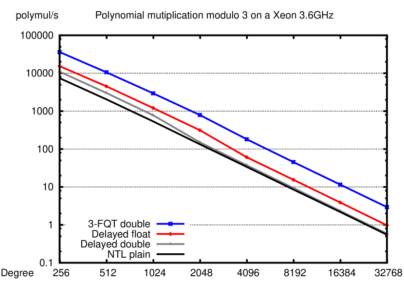
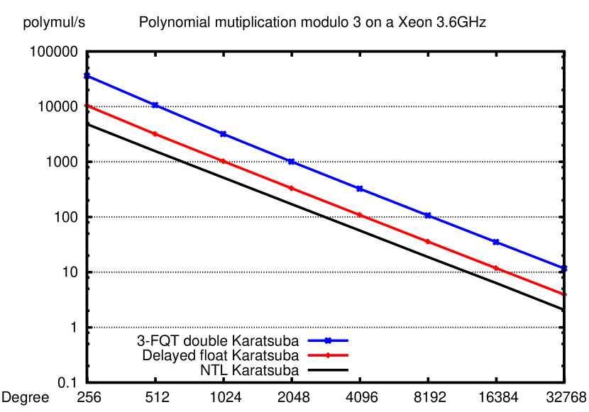
Figure 2: Number of classical and Karatsuba polynomial multiplications modulo 3 per second on a Xeon 3.6 GHz (logarithmic scale)

On Figure 2, we compare our two implementations with that of NTL (Shoup, 2007). We see that the FQT is faster than NTL as long as the same algorithm is used. This shows that our strategy is very useful for small degrees and small primes; not only for the classical algorithm (left) but also for subquadratic ones (right): the use of FQT leads to a gain of an order of magnitude. Note however that in the special case $p=2$, NTL offers a very optimized implementation which is still an order of magnitude faster than our general purpose implementation: specific binary routines, such as the ones proposed by (Weimerskirch et al., 2003), enables to pack coefficients as bits of machine words.

6 Application 2: Small Finite Field Extensions

The isomorphism between finite fields of equal sizes gives a canonical representation: any finite field extension is viewed as the set of polynomials modulo a prime $p$ and modulo an irreducible polynomial ${\cal P}$ of degree $k$. Clearly we can thus convert any finite field element to its $q$-adic expansion; perform the FQT between two elements and then reduce the polynomial thus obtained modulo ${\cal P}$. Furthermore, it is possible to use floating point routines to perform exact linear algebra as demonstrated by Dumas et al. (2009).

We use the strategy of (Dumas et al., 2002, Algorithm 4.1): convert vectors over ${\mathbb{F}}_{p^{k}}$ to $q$-adic floating point; call a fast numerical linear algebra routine (BLAS); convert the floating point result back to the usual field representation. We improve all the conversion steps as follows:

1. replace the Horner evaluation of the polynomials, to form the $q$-adic expansion, by a single table look-up, recovering directly the floating point representation;

2. replace the radix conversion and the costly modular reductions of each polynomial coefficient, by a single REDQ operation;

3. replace the polynomial division by two table look-ups and a single field operation.

Algorithm 6 Fast Dot product over Galois fields via FQT and FQT inverse

0:  A field ${\mathbb{F}}_{p^{k}}$ with elements represented as exponents of a generator of the field;

0:  two vectors $v_{1}$ and $v_{2}$ of elements of ${\mathbb{F}}_{p^{k}}$;

0:  a sufficiently large integer $q$.

0:  $R\in{\mathbb{F}}_{p^{k}}$, with $R=v_{1}^{T}\cdot v_{2}$.
Tabulated $q$-adic conversion
{Use conversion tables from exponent to floating point evaluation}

1:  Set $\widetilde{v_{1}}$ and $\widetilde{v_{2}}$ to the floating point vectors of the evaluations at $q$ of the elements of $v_{1}$ and $v_{2}$.
The floating point computation

2:  Compute $\tilde{r}=\widetilde{v_{1}}^{T}\cdot\widetilde{v_{2}}$;
Computing a radix decomposition

3:  $r=REDQ\_COMPRESSION(\tilde{r},p,q)$;
Variant of REDQ_CORRECTION
{$\mu_{i}$ is such that $\mu_{i}=\widetilde{\mu_{i}}\bmod p$ for $\tilde{r}=\sum_{i=0}^{2k-2}\widetilde{\mu_{i}}q^{i}$}

4:  Set $L=representation(\sum_{i=0}^{k-2}\mu_{i}X^{i})$.

5:  Set $H=representation(X^{k-1}\times\sum_{i=k-1}^{2k-2}\mu_{i}X^{i-k+1})$.
Reduction in the field

6:  Return $R=H+L\in{\mathbb{F}}_{p^{k}}$;

This is presented in Algorithm 6. Line 1 is the table look-up of floating point values associated to elements of the field; line 2 is the numerical computation; line 3 is the first part of the REDQ reduction; lines 4 and 5 are a time-memory trade-off with two table accesses for the corrections of REDQ, combined with a conversion from polynomials to discrete logarithm representation; the last line 6 combines the latter two results, inside the field. A variant of REDQ is used in Algorithm 6, but $u_{i}$ still satisfies $u_{i}=\sum_{j=i}^{2k-2}\mu_{j}q^{j-i}\bmod p$ as shown in Theorem 5. Therefore the representations of $\sum\mu_{i}X^{j}$ in the field can be precomputed and stored in two tables where the indexing will be made by $(u_{0},\ldots,u_{k-1})$ and $(u_{k-1},\ldots,u_{2k-2})$ and not by the $\mu_{i}$’s.

Thus, this algorithm approaches the performance of the prime field wrapping also for small extension fields. Indeed, suppose the internal representation of the extension field is already by discrete logarithms and uses conversion tables from polynomial to index representations (see e.g., Dumas (2004) for details). Then we choose a time-memory trade-off for the REDQ operation of the same order of magnitude, that is to say $p^{k}$. The overall memory required by these new tables only doubles and the REDQ requires only $2$ accesses. Moreover, in the small extension, the polynomial multiplication must also be reduced by an irreducible polynomial, ${\cal P}$. This reduction can be precomputed in the REDQ table look-up and is therefore almost free. Moreover, many things can be factorized if the field representation is by discrete logarithms. For instance, the elements are represented by their discrete logarithm with respect to a generator of the field, instead of polynomials. In this case there are already some table accesses for many arithmetic operations, see e.g., (Dumas, 2004, §2.4) for details.

Theorem 14.

Algorithm 6 is correct.

PROOF. We have to prove that it is possible to compute $L$ and $H$ from the $u_{i}$’s. We have $\mu_{2k-2}=u_{2k-2}$ and $\mu_{i}=u_{i}-qu_{i+1}\bmod p$, for $i=0,\dots,2k-3$. Therefore a precomputed table of $p^{k}$ entries, indexed by $(u_{0},\ldots,u_{k-1})$, can provide the representation of

$$L=\sum_{i=0}^{k-2}(u_{i}-qu_{i+1}\bmod p)X^{i}.$$

Another table with $p^{k}$ entries, indexed by $(u_{k-1},\ldots,u_{2k-2})$, can provide the representation of

$$H=u_{2k-2}X^{2k-2}+\sum_{i=k-1}^{2k-3}(u_{i}-qu_{i+1}\bmod p)X^{i}.$$

Finally $R=X^{k-1}\times\sum_{i={k-1}}^{2k-2}\mu_{i}X^{i-k+1}+\sum_{i=0}^{k-2}\mu_{i}X^{i}$ needs to be reduced modulo the irreducible polynomial used to build the field. But, if we are given the representations of $H$ and $L$ in the field, $R$ is then equal to their sum inside the field, directly using the internal representations.

Table 3 recalls the respective complexities of the conversion phase in both algorithms. Here, $q$ is a power of two and the REDQ division is computed via the floating point routines of Section 4.

	Alg. 1	Alg. 6
Memory	$3p^{k}$	$4p^{k}+2^{1+k\lceil\log_{2}p\rceil}$
Axpy	$0$	$k$
Div	$2k-1$	$0$
Table	$0$	$3$
Red	$\geq 5k$	$1$

Table 3: Complexity of the back and forth conversion between extension field and floating point numbers

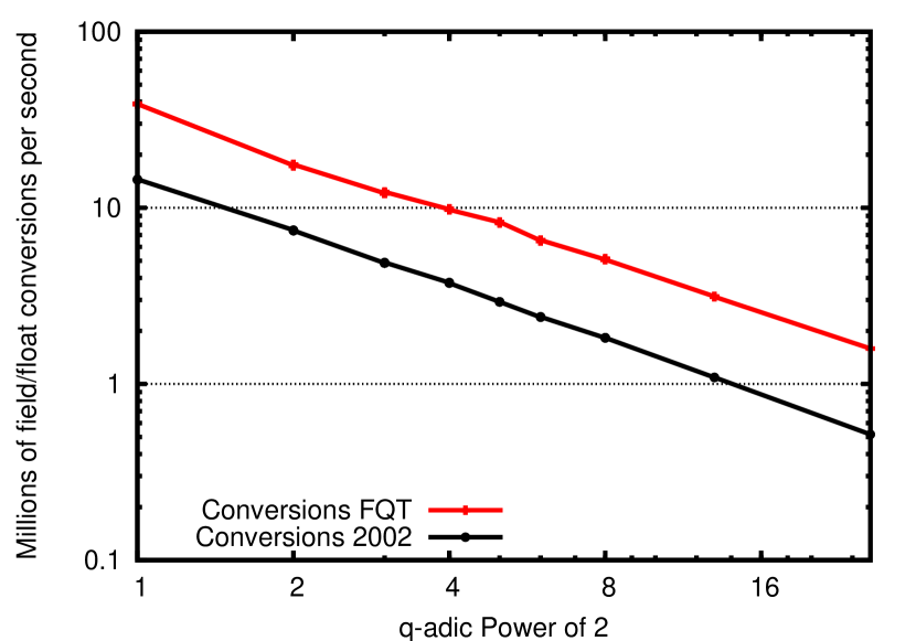
Figure 3: Small extension field conversion speed on a Xeon 3.6GHz

Figure 3 shows the speed of the conversion after the floating point operations. The log scales prove that for $q$ ranging from $2^{1}$ to $2^{26}$ our new implementation is two to three times as fast as the previous one.

Figure 4: Speed of finite field Winograd matrix multiplication on a XEON, 3.6 GHz

Furthermore, these improvements allow the extension field routines to reach the speed of 7800 millions of ${\mathbb{F}}_{9}$ operations per second as shown on Figure 4. The speed-up obtained with these new implementations in also shown on this Figure. It represents a reduction from the 15% overhead of the previous implementation to less than 4% now, when compared over ${\mathbb{F}}_{11}$.

7 Application 3: Compressed Modular Matrix Multiplication

We now extend the results of Dumas et al. (2008) with the REDQ algorithm. The idea is to use Kronecker substitution to pack several matrix entries into a single machine word. We explore the possibilities of packing on the left or on the right only, together with packing on both matrices of a matrix multiplication.

7.1 Middle Product Algorithm

In this section, we show how a dot product of vectors of size $d+1$ can be recovered from a polynomial multiplication performed by a single machine word multiplication. This extends to matrix multiplication by compressing both matrices first. We first illustrate the idea for $2\times 2$ matrices and $d=1$. The product

$$\begin{bmatrix}a&b\\ c&d\\ \end{bmatrix}\times\begin{bmatrix}e&f\\ g&h\\ \end{bmatrix}=\begin{bmatrix}ae+bg&af+bh\\ ce+dg&cf+dh\\ \end{bmatrix}$$

is recovered from

$$\begin{bmatrix}Qa+b\\ Qc+d\\ \end{bmatrix}\times\begin{bmatrix}e+Qg&f+Qh\\ \end{bmatrix}=\begin{bmatrix}*+(ae+bg)Q+*\,Q^{2}&*+(af+bh)Q+*\,Q^{2}\\ *+(ce+dg)Q+*\,Q^{2}&*+(cf+dh)Q+*\,Q^{2}\\ \end{bmatrix},$$

where the character $*$ denotes other coefficients.

Figure 5: Compressed Matrix Multiplication (CMM)

In general, $A$ is an $m\times k$ matrix to be multiplied by a $k\times n$ matrix $B$, the matrix $A$ is first compressed into a $m\times\left\lceil{k}/({d+1})\right\rceil$ CompressedRowMatrix, $CA$, and $B$ is transformed into a $\left\lceil{k}({d+1})\right\rceil\times n$ CompressedColumnMatrix, $CB$. The compressed matrices are then multiplied and the result can be extracted from there. This is depicted on Fig. 5

In terms of number of arithmetic operations, the matrix multiplication $CA\times CB$ can save a factor of $d+1$ over the multiplication of $A\times B$ as shown on the $2\times 2$ case above.

The computation has three stages: compression, multiplication and extraction of the result. The compression and extraction are less demanding in terms of asymptotic complexity, but can still be noticeable for moderate sizes. For this reason, compressed matrices are often reused and it is more informative to distinguish the three phases in an analysis. This is done in Section 7.6 (Table 5), where the actual matrix multiplication algorithm is also taken into account.

Partial compression.

Note that the last column of $CA$ and the last row of $B$ might not have $d+1$ elements if $d+1$ does not divide $k$. Thus one has to artificially append some zeroes to the converted values. On $CB$ this means just do nothing. On $CA$ whose compression is reversed, this means multiplying by $Q$ several times.

7.2 Available Mantissa and Upper Bound on $Q$ for the Middle Product

If the product $CA\times CB$ is performed with floating point arithmetic we just need that the coefficient of degree $d$ fits in the $\beta$ bits of the mantissa. Writing $CA\times CB=c_{H}Q^{d}+c_{L}$, we see that this implies that $c_{H}$, and only $c_{H}$, must have entries that remain smaller than $2^{\beta}$. It can then be recovered exactly by multiplication of $CA\times CB$ with the correctly precomputed and rounded inverse of $Q^{d}$ as shown e.g., in (Dumas, 2008, Lemma 2).

With delayed reduction this means that

$$\sum_{i=0}^{d}\frac{k}{d+1}(i+1)(p-1)^{2}Q^{d-i}<2^{\beta}.$$

On the other hand, delay reduction requires (cf. Eq (3))

$$k(p-1)^{2}<Q.$$ (9)

Thus the recovery is possible if

$$Q^{d+1}<2^{\beta}.$$ (10)

and a single reduction has to be made at the end of the dot product as follows:

Element& init( Element& rem, const double dp) const {
        double r = dp;
        // Multiply by the inverse of Q^d with correct rounding
        r *= _inverseQto_d;
        // Now we just need the part less than Q=2^t
        unsigned long rl( static_cast<unsigned long>(r) );
        rl &= _QMINUSONE;
        // And we finally perform a single modular reduction
        rl %= _modulus;
        return rem = static_cast<Element>(rl);
}

Note that one can avoid the multiplication by the inverse of $Q$ when $Q$ is a power of 2, say $2^{t}$: by adding $Q^{2d+1}$ to the final result one is guaranteed that the $t(d+1)$ high bits represent exactly the $d+1$ high coefficients. On the one hand, the floating point multiplication is then replaced by an addition. On the other hand, this doubles the size of the dot product and thus reduces by a factor of $\sqrt[d+1]{2}$ the largest possible dot product size $k$.

7.3 Middle Product Performance

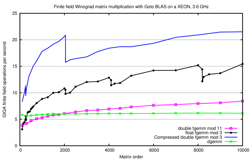
Figure 6: Compressed matrix multiplication compared with dgemm (the floating point double precision matrix multiplication of GotoBlas) and fgemm (the exact routine of FFLAS) with double or single precision.

On Figure 6 we compare our compression algorithm to the numerical double floating point matrix multiplication dgemm of GotoBlas by Goto and van de Geijn (2002) and to the fgemm modular matrix multiplication of the FFLAS-LinBox library by Dumas et al. (2002). For the latter we show timings using dgemm and also sgemm over single floating points. This figure shows that the compression ($d+1$) is very effective for small primes: the gain over the double floating point routine is quite close to $d$.

Observe that the curve of fgemm with underlying arithmetic on single floats oscillates and drops sometimes. Indeed, the matrix begins to be too large and modular reductions are now required between the recursive matrix multiplication steps. Then the floating point BLAS routines are used only when the sub-matrices are small enough. One can see the subsequent increase in the number of classical arithmetic steps on the drops around 2048, 4096 and 8192.

Compression	2	3..4	5..8	8	7	6	5	4	3
Degree d	1	5	9	7	6	5	4	3	2
Q-adic	$2^{3}$	$2^{4}$	$2^{5}$	$2^{6}$	$2^{7}$	$2^{8}$	$2^{10}$	$2^{13}$	$2^{17}$
Dimensions	$2$	$\leq 4$	$\leq 8$	$\leq 16$	$\leq 32$	$\leq 64$	$\leq 256$	$\leq 2048$	$\leq 32768$

Table 4: Compression factors for different common matrix dimensions modulo 3, with $53$ bits of mantissa and $Q$ a power of $2$.

On Table 4, we show the compression factors modulo 3, with $Q$ a power of 2 to speed up conversions. For a dimension $n\leq 256$ the compression is at a factor of five and the time to perform a matrix multiplication is slightly more than a millisecond. Then from dimensions from 257 to 2048 one has a factor of 4 and the times are roughly 16 times the time of the four times smaller matrix. The next stage, from 2048 to 32768 is the one that shows on Figure 5.

Figure 6 shows the dramatic impact of the compression dropping from $4$ to $3$ between $n=2048$ and $n=2049$. It would be interesting to compare the multiplication of $3$-compressed matrices of size $2049$ with a decomposition of the same matrix into matrices of sizes $1024$ and $1025$, thus enabling $4$-compression also for matrices larger than $2048$, but with more modular reductions.

7.4 Right or Left Compressed Matrix Multiplication

Another way of performing compressed matrix multiplication is to multiply an uncompressed $m\times k$ matrix to the right by a row-compressed $k\times{n}/({d+1})$ matrix. We illustrate the idea on $2\times 2$ matrices:

$$\begin{bmatrix}a&b\\ c&d\\ \end{bmatrix}\times\begin{bmatrix}e+Qf\\ g+Qh\\ \end{bmatrix}=\begin{bmatrix}(ae+bg)+Q(af+bh)\\ (ce+dg)+Q(cf+dh)\\ \end{bmatrix}$$

Figure 7: Left, Right and Full Compressions

The general case is depicted on Fig. 7, center. This is called Right Compressed Matrix Multiplication. Left Compressed Matrix Multiplication is obtained by transposition. Here also $Q$ and $d$ must satisfy Eqs. (9) and (10).

The major difference with the Compressed Matrix Multiplication lies in the reductions. Indeed, now one needs to reduce simultaneously the $d+1$ coefficients of the polynomial in $Q$ in order to get the results. This simultaneous reduction can be made by the REDQ algorithm.

When working over compressed matrices $CA$ and $CB$, a first step is to uncompress $CA$, which has to be taken into account when comparing methods. Thus the whole right compressed matrix multiplication is the following algorithm

$$A=\operatorname{Uncompress}(CA);CC=A\times CB;\operatorname{REDQ}(CC)$$ (11)

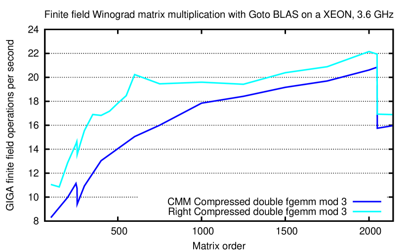
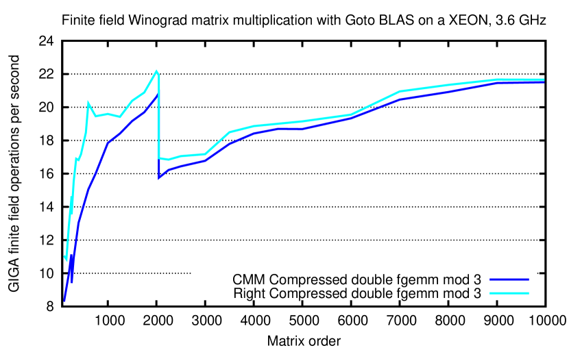
Figure 8: Right Compression and CMM.

We see on Figure 8 that the used of REDQ instead of the middle product algorithm has a high benefit. Indeed for small matrices, the conversion can represent 30% of the time and any improvement there has a high impact.

7.5 Full Compression

It is also possible to compress simultaneously both dimensions of the matrix product (see Fig. 7, right). This is achieved by using polynomial multiplication with two variables $Q$ and $\Theta$. Again, we start by an example in dimension 2:

$$\begin{bmatrix}a+Qc&b+Qd\\ \end{bmatrix}\times\begin{bmatrix}e+\Theta f\\ g+\Theta h\\ \end{bmatrix}=\begin{bmatrix}(ae+bg)+Q(ce+dg)+\Theta(af+bh)+Q\Theta(cf+dh)\\ \end{bmatrix}.$$

More generally, let $d_{q}$ be the degree in $Q$ and $d_{\theta}$ be the degree in $\Theta$. Then, the dot product is:

$$a\cdot b =[\sum_{i=0}^{d_{q}}a_{i0}Q^{i},\dots,\sum_{i=0}^{d_{q}}a_{in}Q^{i}]\times[\sum_{j=0}^{d_{\theta}}b_{0j}\Theta^{j},\dots,\sum_{j=0}^{d_{\theta}}b_{nj}\Theta^{j}],$$

$$=\sum_{l=0}^{k}(\sum_{i=0}^{d_{q}}a_{il})(\sum_{j=0}^{d_{\theta}}b_{lj})Q^{i}\Theta^{j}=\sum_{i=0}^{d_{q}}\sum_{j=0}^{d_{\theta}}(\sum_{l=0}^{k}a_{il}b_{lj})Q^{i}\Theta^{j}.$$

In order to guarantee that all the coefficients can be recovered independently, $Q$ must still satisfy Eq. (9) but then $\Theta$ must satisfy an additional constraint:

$$Q^{d_{q}+1}\leq\Theta.$$ (12)

This imposes restrictions on $d_{q}$ and $d_{\theta}$:

$$Q^{(d_{q}+1)(d_{\theta}+1)}<2^{\beta}.$$ (13)

7.6 CMM Comparisons

In Table 5, we summarize the differences between the algorithms presented on Figures 5 and 7. As usual, the exponent $\omega$ denotes the exponent in the complexity of matrix multiplication. Thus, $\omega=3$ for the classical matrix multiplication, while $\omega<3$ for faster matrix multiplications, as used in (Dumas et al., 2009, §3.2). For products of rectangular matrices, we use the classical technique of first decomposing the matrices into square blocks and then using fast matrix multiplication on those blocks.

7.6.1 Compression Factor

The costs in Table 5 are expressed in terms of a compression factor $e$, that we define as

$$e:=\left\lfloor\frac{\beta}{\log_{2}(Q)}\right\rfloor,$$

where, as above, $\beta$ is the size of the mantissa and $Q$ is the integer chosen according to Eqs. (9) and (10), except for Full Compression where the more constrained Eq. (13) is used.

Thus the degree of compression for the first three algorithms is just $d=e-1$, while it becomes only $d=\sqrt{e}-1$ for the full compression algorithm (with equal degrees $d_{q}=d_{\theta}=d$ for both variables $Q$ and $\Theta$).

Algorithm	Operations	Reductions	Conversions
CMM	$\mathcal{O}\left(mn\left(\frac{k}{e}\right)^{\omega-2}\right)$	$m\times n$ $\operatorname{REDC}$	$\frac{1}{e}mn$ $\operatorname{INIT}_{e}$
Right Comp.	$\mathcal{O}\left(mk\left(\frac{n}{e}\right)^{\omega-2}\right)$	$m\times\frac{n}{e}$ $\operatorname{REDQ}_{e}$	$\frac{1}{e}mn$ $\operatorname{EXTRACT}_{e}$
Left Comp.	$\mathcal{O}\left(nk\left(\frac{m}{e}\right)^{\omega-2}\right)$	$\frac{m}{e}\times n$ $\operatorname{REDQ}_{e}$	$\frac{1}{e}mn$ $\operatorname{EXTRACT}_{e}$
Full Comp.	$\mathcal{O}\left(k\left(\frac{mn}{e}\right)^{\frac{\omega-1}{2}}\right)$	$\frac{m}{\sqrt{e}}\times\frac{n}{\sqrt{e}}$ $\operatorname{REDQ}_{e}$	$\frac{1}{e}mn$ $\operatorname{INIT}_{e}$

Table 5: Number of arithmetic operations for the different algorithms

7.6.2 Analysis

In terms of asymptotic complexity, the cost in number of arithmetic operations is dominated by that of the product (column Operations in the table), while reductions and conversions are linear in the dimensions. This is well reflected in practice. For example, with algorithm Right Compression on matrices of sizes $10,000\times 10,000$ it took $90.73$ seconds to perform the matrix multiplication modulo $3$ and $1.63$ seconds to convert the resulting matrix. This is less than $2$%. For $250\times 250$ matrices it takes less than $0.00216$ seconds to perform the multiplication and roughly $0.0016$ seconds for the conversions. There, the conversions account for $43\%$ of the time and it therefore of extremely high importance to optimize the conversions.

In the case of rectangular matrices, the second column of Table 5 shows that one should choose the algorithm depending on the largest dimension: CMM if the common dimension $k$ is the largest, Right Compression if $n$ if the largest and Left Compression if $m$ dominates. The gain in terms of arithmetic operations is $e^{\omega-2}$ for the first three variants and $e^{\frac{\omega-1}{2}}$ for full compression. This is not only of theoretical interest but also of practical value, since the compressed matrices are then less rectangular. This enables more locality for the matrix computations and usually results in better performance. Thus, even if $\omega=3$, i.e., classical multiplication is used, these considerations point to a source of speed improvement.

The full compression algorithm seems to be the best candidate for locality and use of fast matrix multiplication; however the compression factor is an integer, depending on the flooring of either $\frac{\beta}{\log_{2}(Q)}$ or $\sqrt{\frac{\beta}{\log_{2}(Q)}}$. Thus there are matrix dimensions for which the compression factor of e.g., the right compression will be larger than the square of the compression factor of the full compression. There the right compression will have some advantage over the full compression.

If the matrices are square ($m=n=k)$ or if $\omega=3$, the products all become the same, with similar constants implied in the $O()$, so that apart from locality considerations, the difference between them lies in the time spent in reductions and conversions. Since the $\operatorname{REDQ}_{e}$ reduction is faster than $e$ classical reductions (Dumas, 2008), and since $\operatorname{INIT}_{e}$ and $\operatorname{EXTRACT}_{e}$ are roughly the same operations, the best algorithm would then be one of the Left, Right or Full compression. Further work would include implementing the Full compression and comparing the actual timings of conversion overhead with that of the Right algorithm and that of CMM.

8 Conclusion

We have proposed a new algorithm for simultaneous reduction of several residues stored in a single machine word. For this algorithm we also give a time-memory trade-off implementation enabling very fast running time if enough memory is available.

We have shown very effective applications of this trick for packing residues in large applications. This proves efficient for modular polynomial multiplication, extension fields conversion to floating point and linear algebra routines over small prime fields.

Further work is needed to compare of running times between different choices for $q$. Indeed our experiments were made with $q$ a power of two and large table look-up. With $q$ a multiple of $p$ the table look-up is not needed but divisions by $q^{i}$ will be more expensive. A possibility would be taking $q$ in the form $q=p2^{t}$, then only divisions by $p$ or $p^{i}$ would be made.

It would also be interesting to see in practice how this trick extends to larger precision implementations: on the one hand the basic arithmetic slows down, but on the other hand the trick enables a more compact packing of elements (e.g., if an odd number of field elements can be stored inside two machine words, etc.).

References

- Boldo et al. (2008) Boldo, S., Daumas, M., Giorgi, P., Jul. 2008. Formal proof for delayed finite field arithmetic using floating point operators. In: 8th Conference on Real Numbers and Computers, Santiago de Compostela, Spain. p. 10.
- Coppersmith (1993) Coppersmith, D., Oct. 1993. Solving linear equations over : block Lanczos algorithm. Linear Algebra and its Applications 192, 33–60.
- Dumas (2004) Dumas, J.-G., Jul. 2004. Efficient dot product over finite fields. In: Ganzha, V. G., Mayr, E. W., Vorozhtsov, E. V. (Eds.), Proceedings of the seventh International Workshop on Computer Algebra in Scientific Computing, Yalta, Ukraine. Technische Universität München, Germany, pp. 139–154.
- Dumas (2008) Dumas, J.-G., Jul. 2008. Q-adic transform revisited. In: Jeffrey, D. (Ed.), Proceedings of the 2008 International Symposium on Symbolic and Algebraic Computation, Hagenberg, Austria. ACM Press, New York, pp. 63–69.
- Dumas et al. (2008) Dumas, J.-G., Fousse, L., Salvy, B., May 2008. Compressed modular matrix multiplication. In: Milestones in Computer Algebra 2008, Tobago. p. 8.
- Dumas et al. (2007) Dumas, J.-G., Gautier, T., Giorgi, P., Pernet, C., Roch, J.-L., Villard, G., 2007. Givaro 3.2.9: C++ library for arithmetic and algebraic computations. ljk.imag.fr/CASYS/LOGICIELS/givaro.
- Dumas et al. (2002) Dumas, J.-G., Gautier, T., Pernet, C., Jul. 2002. Finite field linear algebra subroutines. In: Mora, T. (Ed.), Proceedings of the 2002 International Symposium on Symbolic and Algebraic Computation, Lille, France. ACM Press, New York, pp. 63–74.
- Dumas et al. (2004) Dumas, J.-G., Giorgi, P., Pernet, C., Jul. 2004. FFPACK: Finite field linear algebra package. In: Gutierrez, J. (Ed.), Proceedings of the 2004 International Symposium on Symbolic and Algebraic Computation, Santander, Spain. ACM Press, New York, pp. 119–126.
- Dumas et al. (2009) Dumas, J.-G., Giorgi, P., Pernet, C., 2009. Dense linear algebra over word-size prime fields: the FFLAS and FFPACK packages. ACM Transactions on Mathematical Software 35 (3), to appear.
- Gathen and Gerhard (1999) Gathen, J. v., Gerhard, J., 1999. Modern Computer Algebra. Cambridge University Press, New York, NY, USA.
- Goto and van de Geijn (2002) Goto, K., van de Geijn, R., Nov. 2002. On reducing TLB misses in matrix multiplication. Tech. Rep. TR-2002-55, University of Texas, fLAME working note #9, http://www.tacc.utexas.edu/resources/software.
-
Harvey (2007)
Harvey, D., Dec. 24 2007. Faster polynomial multiplication via multipoint
kronecker substitution. ArXiv.org:0712.4046.
URL http://arxiv.org/abs/0712.4046 - Kaltofen and Lobo (1999) Kaltofen, E., Lobo, A., 1999. Distributed matrix-free solution of large sparse linear systems over finite fields. Algorithmica 24 (3-4), 331–348.
- Lefèvre (2005a) Lefèvre, V., 2005a. The Euclidean division implemented with a floating-point division and a floor. Tech. rep., INRIA Rhône-Alpes, http://hal.inria.fr/inria-00000154.
- Lefèvre (2005b) Lefèvre, V., 2005b. The Euclidean division implemented with a floating-point multiplication and a floor. Tech. rep., INRIA Rhône-Alpes, http://hal.inria.fr/inria-00000159.
- LinBox Group (2007) LinBox Group, T., 2007. Linbox 1.1.4: Exact computational linear algebra. www.linalg.org.
- May et al. (2007) May, J. P., Saunders, D., Wan, Z., July 29 – August 1 2007. Efficient matrix rank computation with application to the study of strongly regular graphs. In: Brown, C. W. (Ed.), Proceedings of the 2007 International Symposium on Symbolic and Algebraic Computation, Waterloo, Canada. ACM Press, New York, pp. 277–284.
- Montgomery (1985) Montgomery, P. L., Apr. 1985. Modular multiplication without trial division. Mathematics of Computation 44 (170), 519–521.
- Shoup (2005) Shoup, V., 2005. A computational introduction to number theory and algebra. Cambridge University Press.
- Shoup (2007) Shoup, V., 2007. NTL 5.4.1: A library for doing number theory. www.shoup.net/ntl.
- Weimerskirch et al. (2003) Weimerskirch, A., Stebila, D., Shantz, S. C., 2003. Generic GF(2) arithmetic in software and its application to ECC. In: Safavi-Naini, R., Seberry, J. (Eds.), Information Security and Privacy, 8th Australasian Conference, ACISP 2003, Wollongong, Australia, July 9-11, 2003. Vol. 2727 of Lecture Notes in Computer Science. Springer, pp. 79–92.
-
Weng et al. (2007)
Weng, G., Qiu, W., Wang, Z., Xiang, Q., 2007. Pseudo-Paley graphs and skew
Hadamard difference sets from presemifields. Designs, Codes and
Cryptography 44 (1-3), 49–62.
URL http://dx.doi.org/10.1007/s10623-007-9057-6