Assessment of the RE(OH)₃ Ising-like Magnetic Materials as Possible Candidates for the Study of Transverse-Field-Induced Quantum Phase Transitions

Abstract

The LiHo_xY_1-xF₄ Ising magnetic material subject to a magnetic field, $B_{x}$, perpendicular to the Ho³⁺ Ising direction has shown over the past twenty years to be a host of very interesting thermodynamic and magnetic phenomena. Unfortunately, the availability of other magnetic materials other than LiHo_xY_1-xF₄ that may be described by a transverse field Ising model remains very much limited. It is in this context that we use here mean-field theory to investigate the suitability of the Ho(OH)₃, Dy(OH)₃ and Tb(OH)₃ insulating hexagonal dipolar Ising-like ferromagnets for the study of the quantum phase transition induced by a magnetic field, $B_{x}$, applied perpendicular to the Ising spin direction. Experimentally, the zero field critical (Curie) temperatures are known to be $T_{c}\approx 2.54$ K, $T_{c}\approx 3.48$ K and $T_{c}\approx 3.72$ K, for Ho(OH)₃, Dy(OH)₃ and Tb(OH)₃, respectively. From our calculations we estimate the critical transverse field, $B_{x}^{c}$, to destroy ferromagnetic order at zero temperature to be $B_{x}^{c}=$4.35 T, $B_{x}^{c}=$5.03 T and $B_{x}^{c}=$54.81 T for Ho(OH)₃, Dy(OH)₃ and Tb(OH)₃, respectively. We find that Ho(OH)₃, similarly to LiHoF₄, can be quantitatively described by an effective $S=1/2$ transverse field Ising model (TFIM). This is not the case for Dy(OH)₃ due to the strong admixing between the ground doublet and first excited doublet induced by the dipolar interactions. Furthermore, we find that the paramagnetic (PM) to ferromagnetic (FM) transition in Dy(OH)₃ becomes first order for strong $B_{x}$ and low temperatures. Hence, the PM to FM zero temperature transition in Dy(OH)₃ may be first order and not quantum critical. We investigate the effect of competing antiferromagnetic nearest-neighbor exchange and applied magnetic field $B_{z}$ along the Ising spin direction $\hat{z}$ on the first order transition in Dy(OH)₃. We conclude from these preliminary calculations that Ho(OH)₃ and Dy(OH)₃, and their Y³⁺ diamagnetically diluted variants, Ho_xY_1-x(OH)₃ and Dy_xY_1-x(OH)₃, are potentially interesting systems to study transverse-field induced quantum fluctuations effects in hard axis (Ising-like) magnetic materials.

I Introduction

I.1 Transverse field Ising model

Quantum phase transitions occur near zero temperature and are driven by quantum mechanical fluctuations associated with the Heisenberg uncertainty principle and not by thermal fluctuations as in the case of classical temperature-driven phase transitions Sondhi et al. (1997); Sachdev (1999). There is accumulating evidence that the exotic behavior exhibited by several metallic, magnetic and superconducting materials may have its origin in underlying large quantum fluctuations and proximity to a quantum phase transition. For this reason, much efforts are currently being devoted to understand quantum phase transitions in a wide variety of condensed matter systems.

Perhaps the simplest model that embodies the phenomenon of a quantum phase transition is the transverse field Ising model (TFIM)  Elliott et al. (1970); Chakrabarti et al. (1996), first proposed by de Gennes to describe proton tunneling in ferrolectric materials de Gennes (1963). The spin Hamiltonian for the TFIM reads:

$$H_{{\rm TFIM}} = -\frac{1}{2}\sum_{({\bm{r}}_{i},{\bm{r}}_{j})}J_{ij}(|{\bm{r}}_{j}-{\bm{r}}_{i})|)S_{i}^{z}({\bm{r}}_{i})S_{j}^{z}({\bm{r}}_{j})$$

$$-\Gamma\sum_{({\bm{r}}_{i})}S_{i}^{x}({\bm{r}}_{i}).$$

The ${\bm{S}}_{i}$ ($S=1/2$) quantum spin operators reside on the lattice sites ${\bm{r}}_{i}$ of some $d-$dimensional lattice. The ${\bm{S}}_{i}$ operators are related to the Pauli spin matrices by ${\bm{S}}_{i}=\frac{1}{2}{\bm{\sigma}}_{i}$ (here we set $\hbar=1$). The components of ${\bm{S}}_{i}$ obey the commutation relations $[S_{i}^{\alpha},S_{j}^{\beta}]=i\epsilon_{\alpha\beta\gamma}S_{i}^{\gamma}\delta_{ij}$ where $\alpha$, $\beta$ and $\gamma$ indicate $x$, $y$ and $z$ spin components, $\delta_{ij}$ and $\epsilon_{\alpha\beta\gamma}$ are the Kronecker delta and fully antisymmetric tensor, respectively. $\Gamma$ is the effective transverse field along the $x$ direction, perpendicular to the Ising $z$ axis. As described below, the effective transverse field $\Gamma$ does not correspond one-to-one to the applied physical field $B_{x}$. Rather, $\Gamma$ in Eq. (I.1) is a function of the real physical field $B_{x}$. In fact, $J_{ij}$ is also a function of $B_{x}$  Chakraborty et al. (2004); Tabei et al. (2008a, b). If the spin interactions, $J_{ij}$, possess translational invariance, the system displays for $\Gamma=0$ conventional long range magnetic order below some critical temperature, $T_{c}$. In the simplest scenario, where $J_{ij}>0$, the ordered phase is ferromagnetic and the order parameter is the average magnetization per spin, $m_{z}=(1/N)\sum_{i}\langle S_{i}^{z}\rangle$, where $N$ is the number of spins. Since $S_{i}^{x}$ and $S_{i}^{z}$ do not commute, nonzero $\Gamma$ causes quantum tunneling between the spin-up, $\left|\uparrow\right\rangle$, and spin-down, $\left|\downarrow\right\rangle$, eigenstates of $S_{i}^{z}$. By increasing $\Gamma$, $T_{c}$ decreases until, ultimately, $T_{c}(\Gamma)$ vanishes at a quantum critical point where $\Gamma=\Gamma_{c}$. On the $T=0$ temperature axis, the system is in a long-range ordered phase for $\Gamma<\Gamma_{c}$ while it is in a quantum paramagnetic phase for $\Gamma>\Gamma_{c}$. The phase transition between the paramagnetic and long range ordered phase at $\Gamma_{c}$ constitutes the quantum phase transition Elliott et al. (1970); Chakrabarti et al. (1996).

One can also consider generalizations of the $H_{{\rm TFIM}}$ where the $J_{ij}$ are quenched (frozen) random interactions. Of particular interest is the situation where there are as many ferromagnetic $J_{ij}>0$ and antiferromagnetic $J_{ij}<0$ couplings. This causes a high level of random frustration and the system, provided it is three dimensional, freezes into a spin glass state via a true thermodynamic phase transition at a spin glass critical temperature $T_{g}$ Binder and Young (1986); Mydosh (1993). Here as well, one can investigate how the spin glass transition is affected by a transverse field $\Gamma$. As in the previous example, $T_{g}(\Gamma)$ decreases as $\Gamma$ is increased from zero until, at $\Gamma=\Gamma_{c}$, a quantum phase transition between a quantum paramagnet and a spin glass phase ensues. Extensive numerical studies have found the quantum phase transition between a quantum paramagnet and a spin glass phase Rieger and Young (1994, 1996); Guo et al. (1996) to be quite interesting due to the occurrence of Griffiths-McCoy singularities (GMS) Griffiths (1969); McCoy (1969). These GMS arise from rare spatial regions of disorder which may, for example, resemble the otherwise non-random (disorder-free) version of the system at stake. As a result, GMS can lead to singularities in various thermodynamic quantities away from the quantum critical point.

I.2 LiHo_xY_1-xF₄

On the experimental side, most studies aimed at exploring the phenomena associated with the TFIM have focused on the insulating LiHo_xY_1-xF₄ (LHYF) Ising magnetic material Reich et al. (1990); Wu et al. (1991, 1993); Wu (1992); Bitko et al. (1996); Brooke et al. (1999); Brooke (2000); Ghosh et al. (2002, 2003); Ronnow et al. (2005, 2007); Silevitch et al. (2007a, b); Jönsson et al. (2007); C. Ancona-Torres and Rosenbaum (2008); Jönsson et al. (2008); rec . In this system, the Ho³⁺ Ising spin direction is parallel to the $c$ axis of the body-centered tetragonal structure of LHYF. The random disorder is introduced by diluting the magnetic Ho³⁺ ions by non-magnetic Y³⁺. Crystal field effects lift the degeneracy of the ⁵I₈ electronic manifold, giving an Ising ground doublet $|\Phi_{0}^{\pm}\rangle$ and a first excited $|\Phi_{e}\rangle$ singlet at approximately 11 K above the ground doublet Ronnow et al. (2007). The other 14 crystal field states lie at much higher energies Ronnow et al. (2007). Quantum spin flip fluctuations are introduced by the application of a magnetic field, $B_{x}$, perpendicular to the Ising $c$ axis. $B_{x}$ admixes $|\Phi_{e}\rangle$ with $|\Phi_{0}^{\pm}\rangle$, splitting the latter and producing an effective TFIM with $\Gamma(B_{x})\propto B_{x}^{2}$ for small $B_{x}$ Chakraborty et al. (2004).

The properties of pure LiHoF₄ in a transverse $B_{x}$ are now generally qualitatively well understood Chakraborty et al. (2004). Indeed, a recent quantum Monte Carlo study Chakraborty et al. (2004) found general agreement between experiments and a microscopic model of LiHoF₄. However, some quantitative discrepancies between Monte Carlo and experimental data, even near the classical paramagnetic to ferromagnetic transition where $B_{x}/T_{c}$ is small, do exist  Chakraborty et al. (2004); Tabei et al. (2008a). One noteworthy effect at play in LHYF at low temperatures is the significant enhancement of the zero temperature critical $B_{x}$, $B_{x}^{c}$, caused by the strong hyperfine nuclear interactions in Ho³⁺-based materials Bitko et al. (1996); Ronnow et al. (2005); Chakraborty et al. (2004); Schechter and Stamp (2005).

LiHo_xY_1-xF₄ in a transverse $B_{x}$ and $x<1$ has long been known to display paradoxical behaviors, both in the ferromagnetic (FM) ($0.25<x<1.0$) and spin glass (SG) ($x<0.25$) regimes. In the FM regime, a mean-field behavior $T_{c}(x)\propto x$ for the PM to FM transition is observed when $B_{x}=0$  Brooke et al. (1999). However, in nonzero $B_{x}$, the rate at which $T_{c}(B_{x})$ is reduced by $B_{x}>0$ increases faster than mean-field theory predicts as $x$ is reduced Brooke (2000); Silevitch et al. (2007a). In the high Ho³⁺ (SG) dilution regime (e.g. LiHo_0.167Y_0.833F₄), LHYF has long been Wu et al. (1991, 1993); Jönsson et al. (2007); rec argued to display a conventional SG transition for $B_{x}=0$ signalled by a nonlinear magnetic susceptibility, $\chi_{3}$, diverging at $T_{g}$ as $\chi_{3}(T)\propto(T-T_{g})^{-\gamma}$   Mydosh (1993). However, $\chi_{3}(T)$ becomes less singular as $B_{x}$ is increased from ${B_{x}=0}$, suggesting that no quantum phase transition between a PM and a SG state exists as $T\rightarrow 0$   Wu et al. (1993); Wu (1992). Recent theoretical studies Schechter and Laflorencie (2006); Tabei et al. (2006, 2008b) suggest that for dipole-coupled Ho³⁺ in a diluted sample, nonzero $B_{x}$ generates longitudinal (along the Ising $\hat{z}$ direction) random fields that (i) lead to a faster decrease of $T_{c}(B_{x})$ in the FM regime Brooke (2000); Tabei et al. (2006); Silevitch et al. (2007a) and (ii) destroy the PM to SG transition for samples that otherwise show a SG transition when $B_{x}=0$ Wu et al. (1993); Wu (1992); Jönsson et al. (2007, 2008); rec ; Tabei et al. (2006, 2008b); Schechter and Laflorencie (2006), or, at least, lead to a disappearance of the $\chi_{3}$ divergence as $B_{x}$ is increased from zero Wu et al. (1993); Wu (1992); Tabei et al. (2006).

Perhaps most interesting among the phenomena exhibited by LHYF is the one referred to as antiglass and which has been predominantly investigated in LiHo_0.045Y_0.955F₄  Reich et al. (1990); Ghosh et al. (2003, 2002); Quilliam et al. (2007); Jönsson et al. (2007). The reason for this name comes from AC susceptibility data on LiHo_0.045Y_0.955F₄ which show that the distribution of relaxation times narrows upon cooling below 300 mK  Reich et al. (1990); Ghosh et al. (2002, 2003). This behavior is quite different from that observed in conventional spin glasses where the distribution of relaxation times broadens upon approaching a spin glass transition at $T_{g}>0$  Binder and Young (1986); Mydosh (1993). The antiglass behavior has been interpreted as evidence that the spin glass transition in LiHo_xY_1-xF₄ disappears at some nonzero $x_{c}>0$. Results from more recent experimental studies on LiHo_0.165Y_0.835F₄ ($x=$ 16.5%) and LiHo_0.045Y_0.955F₄ ($x=$ 4.5%) suggest an absence of a genuine spin glass transition, even for a concentration of Ho as large as 16.5%  Jönsson et al. (2007); rec . In particular, it is in stark contrast with theoretical arguments Stephen and Aharony (1981) which predict that, because of the long-ranged $1/r^{3}$ nature of dipolar interactions, classical dipolar Ising spin glasses should have $T_{g}(x)>0$ for all $x>0$. However, even more recent work asserts that there is indeed a thermodynamic SG transition for $x=16.5\%$  C. Ancona-Torres and Rosenbaum (2008), but that the behavior found in LiHo_0.045Y_0.955F₄ is truly unconventional C. Ancona-Torres and Rosenbaum (2008).

Two very different scenarios for the failure of LiHo_0.045Y_0.955F₄ to show a spin glass transition have been put forward Ghosh et al. (2003); Snyder and Yu (2005); Biltmo and Henelius (2007, 2008). Firstly, it has been suggested that the (small) off-diagonal part of the dipolar interactions lead to virtual crystal field excitations that admix $|\Phi_{0}^{\pm}\rangle$ with $|\Phi_{\rm e}\rangle$ and give rise to non-magnetic singlets for spatially close pairs of Ho³⁺ ions. The formation of these singlets would thwart the development of a spin glass state. This mechanism is analogous to the one leading to the formation of the random singlet state in dilute antiferromagnetically coupled $S=1/2$ Heisenberg spins Bhatt and Lee (1982). However, a recent study Chin and Eastham (2006) shows that the energy scale for this singlet formation is very low ($\sim 10^{0}$ mK) and that the random singlet mechanism Ghosh et al. (2003) may not be very effective at destroying the spin glass state in LiHo_0.045Y_0.955F₄  Ghosh et al. (2003). Hence the proposed formation of an entangled state in LiHo_0.045Y_0.955F₄ may, if it really exist, perhaps proceed via a more complex scheme than that proposed in Ref. [Ghosh et al., 2003]. Also, the low-temperature features observed in the specific heat in Ref. [Ghosh et al., 2003] have not been observed in a more recent study Quilliam et al. (2007). Secondly, and from a completely different perspective, numerical simulations of classical Ising dipoles found that the spin glass transition temperature, $T_{g}$ appears to vanish for a concentration of dipoles below approximately 20% of the sites occupied Snyder and Yu (2005); Biltmo and Henelius (2007, 2008). However, even more recent Monte Carlo simulations find that this conclusion may not be that firmly established Tam .

As another possible and yet unexplored scenario, we note here that since Ho³⁺ is an even electron system (i.e. a non-Kramers ion), the Kramers’ theorem is inoperative and the ground state doublet can be split by random (electrostatic) crystal field effects that compete with the collective spin glass behavior. For example, random strains, which may come from the substitution of Ho³⁺$\rightarrow$Y³⁺, break the local tetragonal symmetry and introduces (random) crystal fields operators (e.g. $O_{2}^{\pm 2}$) which have nonzero matrix elements between the two states $|\Phi_{0}^{+}\rangle$ with $|\Phi_{0}^{-}\rangle$ of the ground doublet, splitting it, and possibly destroying the spin glass phase at low Ho³⁺ concentration. Indeed, such random transverse fields have been identified in samples with very dilute Ho³⁺ in a LiYF₄ matrix Shakurov et al. (2005); Bertaina et al. (2006). Also, very weak random strains, hence effective random transverse fields, arise from the different (random) anharmonic zero point motion of ⁶Li and ⁷Li in Ho:LiYF₄ samples with natural abundance of ⁶Li and ⁷Li  Agladze et al. (1991). Finally, there may be intrinsic strains in the crystalline samples that do not arise from the Ho³⁺/Y³⁺ or ⁶Li/⁷Li admisture Shakurov et al. (2005). However, using available estimates Shakurov et al. (2005); Bertaina et al. (2006); Agladze et al. (1991), calculations suggests that strain-induced random fields at play in LiHo_0.045Y_0.955F₄ may be too small [$<O(10^{1}\leavevmode\nobreak\ {\rm mK})$] to cause the destruction of the spin glass phase in this system Fortin and Gingras (2007). Nevertheless, the point remains that, in principle, the non-Kramers nature of Ho³⁺ does offer a route for the destruction of the spin glass phase in LiHo_xY_1-xF₄ outside strictly pairwise, quantum Ghosh et al. (2003); Chin and Eastham (2006) or classical Snyder and Yu (2005); Biltmo and Henelius (2007, 2008), magnetic interaction mechanisms. At this stage, this is clearly a matter that needs to be investigated experimentally further. One notes that, because of Kramers’ theorem, the destruction of a SG phase via strain-induced effective random transverse fields would not occur for an odd-electron (Kramers) ion such as Dy³⁺ or Er³⁺. In that context, one might think that a comparison of the behavior of LiDy_xY_1-xF₄ or LiEr_xY_1-xF₄ with that of LiHo_xY_1-xF₄ would be interesting. Unfortunately, while LiHo_xY_1-xF₄ is an Ising system, the Er³⁺ and Dy³⁺ moments in LiEr_xY_1-xF₄ and LiDy_xY_1-xF₄ are XY-like Magarino et al. (1980); Kazei et al. (2006). Hence, one cannot compare the LiEr_xY_1-xF₄ and LiDy_xY_1-xF₄ XY compounds with the LiHo_xY_1-xF₄ Ising material on the same footing.

From the above discussion, it is clear that there are a number of fundamental questions raised by experimental studies of LiHo_xY_1-xF₄, both in zero and nonzero transverse field $B_{x}$, that warrant systematic experimental investigations in other similar diamagnetically-diluted dipolar Ising-like magnetic materials. Specific questions are:

1. How does the quantum criticality of a transverse field Ising material with much smaller hyperfine interactions than Ho³⁺ in LiHo_xY_1-xF₄ manifest itself Bitko et al. (1996); Ronnow et al. (2005); Schechter and Stamp (2005) ?

2. Is the theoretical proposal of transverse-induced random longitudinal fields in diluted dipolar Ising materials Tabei et al. (2006); Schechter and Laflorencie (2006); Tabei et al. (2008b) valid and can it be explored and confirmed in other materials other than LiHo_xY_1-xF₄ Silevitch et al. (2007a)? In particular, are the phenomena observed in Ref. [Silevitch et al., 2007a] and ascribed to Griffiths singularities observed in other disordered dipolar Ising systems subject to a transverse field?

3. Does the antiglass phenomenon Reich et al. (1990); Ghosh et al. (2002, 2003) occur in other diluted dipolar Ising materials? If yes, which, if any, of the aforementioned theoretical proposals for the destruction of the spin glass state at small spin concentration is correct?

I.3 RE(OH)₃ materials

As mentioned above, these questions cannot be investigated with the LiEr_xY_1-xF₄ and LiDy_xY_1-xF₄ materials isotructural to the LiHo_xY_1-xF₄ Ising compound since they are XY-like systems. However, we note in passing that it would nevertheless be interesting to explore the topic of induced random fields Schechter and Laflorencie (2006); Tabei et al. (2006, 2008b) and the possible existence of an XY dipolar spin glass and/or antiglass state in LiEr_xY_1-xF₄ and LiDy_xY_1-xF₄. The LiTb_xY_1-xF₄ material is of limited use in such investigations since the single ion ground state of Tb³⁺ in this compound consists of two separated singlets Liu et al. (1988), and local moment magnetism on the Tb³⁺ site disappears at low Tb concentration Aeppli (1998). In this paper, we propose that the RE(OH)₃ (RE=Ho, Dy) compounds may offer themselves as an attractive class of materials to study the above questions. Similarly to the LiHoF₄, the RE(OH)₃ materials possess the following interesting properties:

1. They are insulating rare earth materials.

2. Their main spin-spin couplings are magnetostatic dipole-dipole interactions.

3. The RE(OH)₃ materials are stable at room temperature.

4. Both pure RE(OH)₃ and LiHoF₄ are colinear (Ising-like) dipolar ferromagnets with the Ising direction along the $c$ axis of a hexagonal unit cell (RE(OH)₃) or body-centered tetragonal unit cell (LiHoF₄). In both cases there are two magnetically equivalent ions per unit cell.

5. In RE(OH)₃, the Kramers (Dy³⁺) and non-Kramers (Ho³⁺) variants possess a common crystalline structure and both have similar bulk magnetic properties in zero transverse magnetic field $B_{x}$.

6. The critical temperature of the pure RE(OH)₃ compounds is relatively high, $\sim 3\leavevmode\nobreak\ {\rm K}$. This would make possible the study of Y$-$substituted Dy and Ho hydroxides down to quite low concentration of rare earth while maintaining the relevant magnetic temperature scale above the lowest attainable temperature with a commercial dilution refrigerator.

7. Finally, and this is a key feature that motivated the present study, the first excited crystal field state in the Ho(OH)₃ and Dy(OH)₃ compounds is low-lying, hence allowing a possible transverse-field induced admixing and, possibly, a transverse field Ising model description spi

To the best of our knowledge, it appears that the RE(OH)₃ materials have so far not been investigated as potential realization of the TFIM. The purpose of this paper is to explore (i) the possible description of these materials as a TFIM, (ii) obtain an estimate of what the zero temperature critical transverse field $B_{x}^{c}$ may be and, (iii) assess if any new interesting phenomenology may occur, even in the pure compounds, in nonzero transverse field $B_{x}$.

We note, however, that there are so far no very large single crystals of RE(OH)₃ available Catanese et al. (1973). For example, their length typically varies between 3 mm and 17 mm and their diameter between 0.2 and 0.6 mm. The lack of large single crystals would make difficult neutron scattering experiments. However, possibly motivated by this work and by a first generation of bulk measurements (e.g. susceptibility, specific heat), experimentalists and solid state chemists may be able to conceive ways to grow larger single crystals of RE(OH)₃. Also, in light of the fact that most experiments on LiHo_xY_1-xF₄ that have revealed exotic behavior are bulk measurements Reich et al. (1990); Wu et al. (1991, 1993); Brooke et al. (1999); Ghosh et al. (2002, 2003); Quilliam et al. (2007), we hope that at this time the lack of availability of large single crystals of the RE(OH)₃ series is not a strong impediment against pursuing a first generation of bulk experiments on RE(OH)₃.

The rest of this paper is organized as follows. In Section II, we review the main, single ion, magnetic properties of RE(OH)₃ (RE=Dy, Ho, Tb). In particular, we discuss the crystal field Hamiltonian of these materials and the dependence of the low-lying crystal field levels on an applied transverse field $B_{x}$. We present in Section III a mean-field calculation to estimate the $B_{x}$ vs temperature, $T$, $T_{c}(B_{x})$ phase diagram of these materials. In Section IV, we show that Ho(OH)₃ and Tb(OH)₃ can be described quantitatively well by a transverse field Ising model, while Dy(OH)₃ cannot. The Subsection A of Section V, uses a Ginzburg-Landau theory to explore the first order paramagnetic (PM) to ferromagnetic (FM) transition that occurs in Dy(OH)₃ at low temperatures and strong $B_{x}$. The following Subsection B discusses the effect of nearest-neighbor antiferromagnetic exchange interaction and applied longitudinal (i.e. along the $\hat{z}$ axis) magnetic field, $B_{z}$, on the first order transition in Dy(OH)₃. A brief conclusion is presented in Section VI. Appendix A discusses how the excited crystal field states in Dy(OH)₃ play an important quantitative role on the determination of $T_{c}(B_{x})$ in this material.

II RE(OH)₃: Material properties

II.1 Crystal properties

All the rare earth hydroxides form hexagonal crystals that that are iso-structural with Y(OH)₃. The lattice is described by translation vectors $\bm{a_{1}}=(0,0,0)$, $\bm{a_{2}}=(-a/2,a\sqrt{3}/2,0)$ and $\bm{a_{3}}=(0,0,c)$. A unit cell consist of two Ho³⁺ ions at coordinates $(1/3,2/3,1/4)$ and $(2/3,1/3,3/4)$ in the basis of lattice vectors $\bm{a_{1}}$, $\bm{a_{2}}$ and $\bm{a_{3}}$. The coordinates of three O^2- and H^- ions, relative to the position of Ho³⁺, are $\pm(x,y,0)$, $\pm(-y,x-y,0)$ and $\pm(y-x,-x,0)$, where $\pm$ refers to the first and second Ho³⁺ in the unit cell, respectively Scott (1970). The values of the parameters x and y are listed in Table 1. x=0.396, y=0.312 and for H^-: x=0.28, y=0.17Beall et al. (1977). The lattice structure is depicted in Fig. 1. The lattice constants for Tb(OH)₃, Dy(OH)₃, Ho(OH)₃ and Y(OH)₃, from Beall et al. Beall et al. (1977), are collected in Table 2. Each magnetic ion is surrounded by 9 oxygen atoms that create a crystalline field characterized by the point group symmetry $C_{3h}$Scott (1970).

	O2-, $x$	O2-, $y$	H-, $x$	H-, $y$
Tb(OH)3	$0.3952(7)$	$0.3120(6)$	$0.276(1)$	$0.142(1)$
Dy(OH)3	$0.3947(6)$	$0.3109(6)$	$0.29(3)$	$0.15(2)$
Ho(OH)3	$0.3951(7)$	$0.3112(7)$	$0.30(3)$	$0.17(3)$
Y(OH)3	$0.3958(6)$	$0.3116(6)$	$0.28(1)$	$0.17(1)$

Table 1: Position parameters of O^2- and H^- ions in rare earth hydroxides and Y(OH)₃ from Ref. [Beall et al., 1977] and Ref. [Landers and Brun, 1973] (see text in Section II.1).

	$a$	$c$	$c/a$
Tb(OH)3	$6.315(4)$	$3.603(2)$	$0.570(5)$
Dy(OH)3	$6.286(3)$	$3.577(1)$	$0.569(0)$
Ho(OH)3	$6.266(2)$	$3.553(1)$	$0.567(0)$
Y(OH)3	$6.261(2)$	$3.544(1)$	$0.566(0)$

Table 2: Lattice constants for rare earth hydroxides and Y(OH)₃ (from Ref. [Beall et al., 1977]).

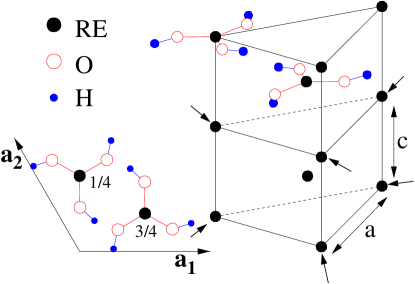
Figure 1: The lattice structure of rare earth hydroxides and Y(OH)₃. The arrows indicate the 6 nearest neighbors of the central ion in the lower prism. The lower left corner shows a projection of the unit cell onto the plane given by lattice vectors $\bm{a_{1}}$ and $\bm{a_{2}}$.

II.2 Single ion properties

The electronic configuration of the magnetic ions Tb³⁺, Dy³⁺ and Ho³⁺ is, respectively, $4f^{8}$, $4f^{9}$ and $4f^{10}$. Magnetic properties of the rare earth ions can be described by the states of the lowest energy multiplet: the spin-obit splitting between the ground state $J$ manifold and the first excited states is of order of few thousands K. The ground state manifolds can be found from Hund’s rules and are ${}^{7}F_{6}$, ${}^{6}H_{15/2}$ and ${}^{5}I_{8}$ for Tb³⁺, Dy³⁺ and Ho³⁺, respectively. The Wigner-Eckart theorem gives the Landé $g$-factor equal to $\frac{3}{2}$, $\frac{4}{3}$ and $\frac{5}{4}$ for Tb³⁺, Dy³⁺ and Ho³⁺, respectively.

In a crystalline environment, an ion is subject to the electric field and covalency effects from the surrounding ions. This crystalline field effect partially lifts the degeneracy of the ground state multiplet. The low energy levels of Tb³⁺ in Tb(OH)₃ are a pair of singlets, that consist of the symmetric combination of $\left|\pm 6\right\rangle$ states with a small admixture of the $\left|0\right\rangle$ state and an antisymmetric combination 0.3 cm^-1 above Scott et al. (1969). The next excited state is well separated from the lowest energy pair by an energy of 118 cm^-1  Scott et al. (1969) (1 cm${}^{-1}\approx 1.44$ K). In the case of Dy³⁺ in Dy(OH)₃, the spectrum consist of 8 Kramers doublets with the first excited state 7.8 cm^-1 above the ground state Kahle et al. (1986). The low energy spectrum of Ho³⁺ in Ho(OH)₃ is composed of a ground state doublet and an excited singlet state 11.1 cm^-1 above Scott (1970).

Due to the strong shielding of the $4f$ electrons by the electrons of the filled outer electronic shells, the exchange interactions for $4f$ electrons is weak and the crystal field can be considered as a perturbation to the fixed $J$ manifold. Furthermore, because the strong spin-obit interaction yields a large energy gap between the ground state multiplet and the excited levels, we neglect all the excited electronic multiplets in the calculation.

According to arguments provided by Stevens Stevens (1952), we express the matrix elements of the crystal field Hamiltonian for the ground state manifold in terms of operator equivalents. The details of the method and conventions for expressing the crystal field Hamiltonian can be found in the review by Hutchings Hutchings (1964). On the basis of the Wigner-Eckart theorem, one can write the crystal field Hamiltonian in the form

$$\mathcal{H}_{\rm cf}=\sum_{nm}\theta_{n}B_{n}^{m}O_{n}^{m},$$ (2)

where $O_{n}^{m}$ are Steven’s “operator equivalents”, $\theta_{n}$ are constants called Stevens multiplicative factors and $B_{n}^{m}$ are crystal field parameters (CFP). The CFP are usually determined by fitting experimental (spectroscopic) data. From angular momentum algebra, we know that in the case of f electrons, we need to consider only $n=0,2,4,6$ in the sum (2). The choice of $B_{n}^{m}$ coefficients in Hamiltonian (2) that do not vanish and have nonzero corresponding matrix elements is dictated by the point symmetry group of the crystalline environment. The Stevens operators, $O_{n}^{m}$, are conveniently expressed in terms of vector components of angular momentum operator ${\bm{J}}$. In the case of the RE(OH)₃ materials, considered herein, the point-symmetry group is $C_{3h}$, and the crystal field Hamiltonian is of the form

$${\cal H}_{\rm cf}({{\bm{J}}}_{i}) = \alpha_{J}B_{2}^{0}O_{2}^{0}({{\bm{J}}}_{i})+\beta_{J}B_{4}^{0}O_{4}^{0}({{\bm{J}}}_{i})$$ (3)

$$+\gamma_{J}B_{6}^{0}O_{6}^{0}({{\bm{J}}}_{i})+\gamma_{J}B_{6}^{6}O_{6}^{6}({{\bm{J}}}_{i}).$$

The Stevens multiplicative factors $\alpha_{J}$, $\beta_{J}$ and $\gamma_{J}$ ($\theta_{2}$, $\theta_{4}$ and $\theta_{6}$) are collected in Table. 3.

Ion	$\alpha_{J}$	$\beta_{J}$	$\gamma_{J}$
Tb3+	$-1/(3^{2}\cdot 11)$	$2/(3^{3}\cdot 5\cdot 11^{2})$	$-1/(3^{4}\cdot 7\cdot 11^{2}\cdot 13)$
Dy3+	$-2/(3^{2}\cdot 5\cdot 7)$	$-2^{3}/(3^{3}\cdot 5\cdot 7\cdot 11\cdot 13)$	$2^{2}/(3^{3}\cdot 7\cdot 11^{2}\cdot 13^{2})$
Ho3+	$-1/(2\cdot 3^{2}\cdot 5^{2})$	$-1/(2\cdot 3\cdot 5\cdot 7\cdot 11\cdot 13)$	$-5/(3^{3}\cdot 7\cdot 11^{2}\cdot 13^{2})$

Table 3: Stevens multiplicative factors

Ref	Crystal	$B_{2}^{0}$(cm-1)	$B_{4}^{0}$(cm-1)	$B_{6}^{0}$(cm-1)	$B_{6}^{6}$(cm-1)
Scott (1970)	Tb(OH)3*	$207.9\pm 2.8$	$-69.0\pm 1.6$	$-45.3\pm 1.1$	$585\pm 10$
Scott (1970)	Tb:Y(OH)3	$189.1\pm 2.6$	$-69.1\pm 1.5$	$-45.7\pm 1.0$	$606\pm 9$
Scott (1970)	Dy(OH)3*	$209.4\pm 3.4$	$-75.5\pm 3.5$	$-40.1\pm 1.9$	$541.8\pm 26.5$
Karmakar et al. (1981)	Ho(OH)3	$200\pm 2.0$	$-57\pm 0.5$	$-40\pm 0.5$	$400\pm 5$
Scott (1970)	Ho:Y(OH)3*	$246.0\pm 3.4$	$-56.7\pm 1.2$	$-39.8\pm 0.3$	$543.6\pm 3.3$
Karmakar et al. (1982)	Dy(OH)3	$215.9$	$-72.0$	$-42.0$	$515.3$

Table 4: Crystal field parameters. Some of the calculation we performed with one set of crystal field parameters only. Crystal field parameters arbitrary chosen Arb to be used in these calculations are marked with *.

For the sake of conciseness, and to illustrate the procedure, most of our numerical results below are presented for one set of CFP only. The qualitative picture that emerges from our calculatiosn does not depend on the specific choice of CFP parameters. Only quantitative differences are found using the different sets of CFP. Ultimately, a further experimental determination of accurate $B_{n}^{m}$ values would need to be carried out in order to obtain more precise mean-field estimates as well as to perform quantum Monte Carlo simulations of the Re(OH)₃ systems. According to our arbitrary choice Arb , if not stated otherwise, we use in the calculations the CFP provided by Scott et al. Scott (1970); Scott and Wolf (1969); Kahle et al. (1986); Scott et al. (1969). For Ho(OH)₃ and Dy(OH)₃ different values of CFP were proposed by Karmakar et al. Karmakar et al. (1981, 1982). As one can see in Fig. 3, for Ho(OH)₃, the latter set of CFP yields a somewhat higher mean-field critical temperature and quite a bit higher critical value of the transverse magnetic field $B_{x}^{c}=$7.35 T, compared with $B_{x}^{c}=$4.35 T obtained using Scott et al.’s CFP Scott (1970)(see Fig. 3). Similarly, Karmakar et al.’s CFP  Karmakar et al. (1982) for Dy(OH)₃ give a much higher critical field of $B_{x}^{c}=$9.12 T, compared with $B_{x}^{c}=$ 5.03 T when Scott ’s et al.’s CFP Scott (1970); Scott and Wolf (1969); Kahle et al. (1986) are used. From the two sets of CFP for Tb(OH)₃ we choose the one obtained from measurements on pure Tb(OH)₃ Scott (1970). Using the CFP obtained for the system with a dilute concentration of Tb in a Y(OH)₃ matrix, Tb:Y(OH)₃ Scott (1970), makes only a small change to the value of critical transverse field; we obtained $B_{x}^{c}=$50.0 T and $B_{x}^{c}=$54.8 T calculated using Tb:Y(OH)₃ and Tb(OH)₃ CFP, respectively (see Fig. 3). Available values of the CFP are given in Table 4.

Eigenstate	Energy $[cm^{-1}]$
Dy(OH)3
$0.92\left|\pm 15/2\right\rangle-0.15\left|\pm 3/2\right\rangle+0.37\left|\mp 9/2\right\rangle$
$0.40\left|\pm 15/2\right\rangle+0.20\left|\pm 3/2\right\rangle-0.90\left|\mp 9/2\right\rangle$	9.6
Dy(OH)3 Karmakar et al., Ref. [Karmakar et al., 1981, 1982]
$0.98\left|\pm 15/2\right\rangle-0.09\left|\pm 3/2\right\rangle+0.15\left|\mp 9/2\right\rangle$
$0.17\left|\pm 15/2\right\rangle+0.22\left|\pm 3/2\right\rangle-0.96\left|\mp 9/2\right\rangle$	19.3
Ho:Y(OH)3
$0.94\left|\pm 7\right\rangle+0.31\left|\pm 1\right\rangle+0.15\left|\mp 5\right\rangle$
$0.59\left|6\right\rangle+0.55\left|0\right\rangle+0.59\left|-6\right\rangle$	12.7
Ho(OH)3 Karmakar et al., Ref. [Karmakar et al., 1981, 1982]
$0.97\left|\pm 7\right\rangle+0.24\left|\pm 1\right\rangle+0.09\left|\mp 5\right\rangle$
$0.60\left|6\right\rangle+0.52\left|0\right\rangle+0.60\left|-6\right\rangle$	23.6
Tb(OH)3
$0.71\left|6\right\rangle+0.05\left|0\right\rangle+0.71\left|-6\right\rangle$
$0.71\left|6\right\rangle-0.71\left|-6\right\rangle$	0.49
$0.99\left|\pm 5\right\rangle+0.13\left|\mp 1\right\rangle$	122.06
Tb:Y(OH)3
$0.71\left|6\right\rangle+0.06\left|0\right\rangle+0.71\left|-6\right\rangle$
$0.71\left|6\right\rangle-0.71\left|-6\right\rangle$	0.58
$0.99\left|\pm 5\right\rangle+0.16\left|\mp 1\right\rangle$	115.33

Table 5: Eigenstates and energy levels calculated with the crystal field parameters collected in Table 4.

We show in Table 5 the lowest eigenstates and eigenvalues of the crystal field Hamiltonian (3). The calculated energies are not in full agreement with the experimentally determined values because the CFP were fitted using all the observed optical transitions, including transitions between diffent ${\bm{J}}$ manifolds Scott (1970). Furthermore, the fitting procedure used by Scott Scott (1970) includes perturbative admixing between manifolds with the admixing incorporated into effective Stevens multiplicative factors $\alpha_{J}$, $\beta_{J}$ and $\gamma_{J}$ that slightly differ from those given in Table  3.

Given the uncertainty in the CFP, which ultimately lead to an uncertainty of approximately $\sim 40\%$ on $B_{x}^{c}$ in Ho(OH)₃ and Dy(OH)₃, as well as the nature of the mean-field calculations that we use and which neglects thermal and quantum mechanical fluctuations, as well as for simplicity sake, we ignore here the effect of hyperfine coupling of the electronic and nuclear magnetic moments. However, as shown for LiHo_xY_1-xF₄, the important role of hyperfine interactions for Ho³⁺ on the precise determination of $B_{x}^{c}$ must eventually be considered Bitko et al. (1996); Chakraborty et al. (2004); Ronnow et al. (2005); Schechter and Stamp (2005). At this time, one must await results from further experiments and a precise set of CFP for ${\cal H}_{c}$ in order to go beyond the mean-field calculations presented below or to pursue quantum Monte Carlo calculations as done in Refs. [Chakraborty et al., 2004; Tabei et al., 2008a]. As suggested in Ref. [Chakraborty et al., 2004], the accuracy of any future calculations (mean-field or quantum Monte Carlo) could be improved by the use of directly measured accurate values of the transverse field splitting of the ground state doublet instead of the less certain values calculated from CFP.

Since our main goal in this exploratory work is to estimate the critical transverse field, $B_{x}^{c}$, for the family of RE(OH)₃ compounds and to explore the possible validity of a transverse field Ising model description of these materials, we henceforth restrict ourselves to the ${\cal H}_{\rm cf}$ in Eq. (2) with the CFP ($B_{n}^{m}$ parameter values) given in Table  4. These calculations could be revisited and quantum Monte Carlo simulations Chakraborty et al. (2004); Tabei et al. (2008a) performed once experimental results reporting on the effect of $B_{x}$ on Dy(OH)₃ and Ho(OH)₃ become available.

II.3 Single ion transverse field spectrum

A magnetic field, $B_{x}$, applied in the direction transverse to the easy axis splits the degeneracy of the ground state doublet in the case of Ho(OH)₃ and Dy(OH)₃, or increase the separation of the ground levels in the case of the already weakly separated singlets in Tb(OH)₃. By diagonalizing the single-ion Hamiltonian, ${\cal H}_{0}$, which consist of the crystal field and Zeeman term,

$$\mathcal{H}_{0}={\cal H}_{\rm cf}({\bm{J}}_{i})-g\mu_{\rm B}B_{x}J_{x},$$ (4)

we obtain the transverse field dependence of the single ion energy levels, plotted in Fig. 2. In the case of Dy(OH)₃, the two lowest energy levels splitting is too small to be clearly visible in the main panel of Fig. 2. Hence, we show the energy separation between the two lowest levels in the inset of Fig. 2 for Dy(OH)₃. Furthermore, the separation vanishes at $B_{x}=3.92$ T, indicating that the two lowest states for this specific value of the transverse field, $B_{x}$, are degenerate.

To calculate the transverse field dependence of the lowest energy levels up to the critical transverse field where dipolar ferromagnetism is destroyed, we do not have to include all the crystal field states since the $B_{x}$-induced admixing among the states decreases with increasing energy separation. In the case of Ho(OH)₃ we can reproduce the field dependence, $B_{x}$, of the lowest energy levels, $E$ in Fig. 2 using only the four lowest levels. However, in order to achieve a similar level of agreement for Dy(OH)₃, we have to retain the ground doublet and several of the lowest excited doublets.

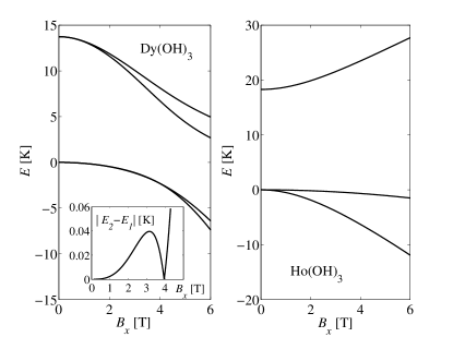
Figure 2: Energy levels as a function of applied transverse field for Dy(OH)₃ and Ho(OH)₃ . The inset shows the separation of the lowest energy levels in Dy(OH)₃.

III Numerical solution

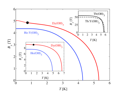
Figure 3: The main panel shows the phase diagrams for Dy(OH)₃ and Ho:Y(OH)₃ (crystal field parameters of Scott et al. Scott (1970); Kahle et al. (1986)). The dot indicates the location of the tricritical point for Dy(OH)₃. The transition is first order for temperatures below the temperature location of the tricritical point. The upper inset shows the phase diagram for Tb(OH)₃ (crystal field parameters of Scott et al. Scott (1970); Scott et al. (1969); Scott and Wolf (1969)). The lower inset shows the phase diagram for Ho(OH)₃ and Dy(OH)₃ calculated with the crystal field parameters of Karmakar et al. Karmakar et al. (1981, 1982).

The collective magnetic properties of the considered rare earth hydroxides are mainly controlled by a long range dipolar interaction between the magnetic moments carried by the rare earth ions. The dipolar interaction is complemented by a short range exchange interaction. Adding the interaction terms to the single ion Hamiltonian (4) gives a full Hamiltonian, ${\cal H}$, of the form

$$\mathcal{H} = \sum_{i}{\cal H}_{\rm cf}({\bm{J}}_{i})-g\mu_{\rm B}\sum_{i}B_{x}J_{i,x}$$ (5)

$$+ \frac{1}{2}\sum_{ij}\sum_{\mu\nu}\mathcal{L}_{ij}^{\mu\nu}J_{i,\mu}J_{j,\nu}+\frac{1}{2}\mathcal{J_{{\rm ex}}}\sum_{i,nn}{\bm{J}}_{i}\cdot{\bm{J}}_{nn}.$$

$\mathcal{L}_{ij}^{\mu\nu}$ are the anisotropic dipole-dipole interaction constants of the form $\mathcal{L}_{ij}^{\mu\nu}=\frac{\mu_{0}(g\mu_{\rm B})^{2}}{4\pi a^{3}}L_{ij}^{\mu\nu}$, where $\mu,\nu=x,y,z$; $a$ is a lattice constant (see Table 2) and $\mu_{0}$ is the permeability of vacuum. $L_{ij}^{\mu\nu}$ are dimensionless dipolar interaction coefficients,

$$L_{ij}^{\mu\nu}=\frac{\delta^{\mu\nu}\left|{\bm{r}}_{ij}\right|^{2}-3\left({\bm{r}}_{ij}\right)^{\mu}\left({\bm{r}}_{ij}\right)^{\nu}}{\left|{\bm{r}}_{ij}\right|^{5}},$$ (6)

where ${\bm{r}}_{ij}={\bm{r}}_{j}-{\bm{r}}_{i}$, with ${\bm{r}}_{i}$ the lattice position of magnetic moment ${\bm{J}_{i}}$, expressed in units of the lattice constant, $a$. $\mathcal{J_{{\rm ex}}}$ is the antiferromagnetic ($\mathcal{J_{{\rm ex}}}>0$) exchange interaction constant, which can be recast as $\mathcal{J_{{\rm ex}}}=\frac{\mu_{0}(g\mu_{\rm B})^{2}}{4\pi a^{3}}J_{{\rm ex}}$, where $J_{{\rm ex}}$ is now a dimensionless exchange constant that, when multiplied by the nearest neighbor coordination number, $z$=6, can be use to compare the relative strength of exchange vs the magnetic dipolar lattice sum (energies) collected in Table 6. The label $nn$ in Eq. (5) denotes the nearest neighbor sites of site $i$.

The exchange interaction is expected to be of somewhat lower strength than the dipolar coupling Catanese and Meissner (1973); Catanese et al. (1973). We therefore neglect it in most of the calculations, but we discuss its effect on the calculated $B_{x}$ vs $T$ phase diagram at the end of this section as well as explore its influence on the occurrence of a first order phase transition in Dy(OH)₃ in Section V.2. Denoting $L_{\mu\nu}=\sum_{j}L_{ij}^{\mu\nu}$ and $\mathcal{L}_{\mu\nu}=\frac{\mu_{0}(g\mu_{\rm B})^{2}}{4\pi a^{3}}L_{\mu\nu}$, we write a mean-field Hamiltonian in the form

$$\mathcal{H}_{\rm MF} = {\cal H}_{c}({\bm{J}})-g\mu_{\rm B}B_{x}J_{x}$$ (7)

$$+ \sum_{\mu=x,y,z}\left(\mathcal{L}_{\mu\mu}+z{\cal J}_{\rm ex}\right)\left(J_{\mu}\left\langle J_{\mu}\right\rangle-\frac{1}{2}\left\langle J_{\mu}\right\rangle^{2}\right).$$

with $z=6$ the number of nearest neighbors. The last term in Eq. (7), $-\frac{1}{2}\left\langle J_{\mu}\right\rangle^{2}$, has no effect on the calculated thermal expectation values of the $\hat{x}$ and $\hat{z}$ components of the magnetization, and can be dropped. The off-diagonal terms, $\mathcal{L}_{\mu\nu}$ with $\mu\neq\nu$, vanish due to the lattice symmetry. We employ the Ewald technique Ewald (1921); Ziman (1972); de Leeuw et al. (1980); Born and Huang (1968); Melko and Gingras (2004) to calculate the dipole-dipole interaction, $L_{ij}^{\mu\nu}$, of Eq. (6). By summing over all sites $j$ coupled to an arbitrary site $i$, we obtain the coefficients $L_{\mu\nu}$ listed in Table 6. The considered Ewald sums ignore a demagnetization term Melko and Gingras (2004) and our calculations can therefore be interpreted as corresponding to a long needle-shape sample.

	$L_{xx}$	$L_{yy}$	$L_{zz}$
Tb(OH)3	-11.43	-11.43	-28.01
Dy(OH)3	-11.40	-11.41	-28.20
Ho(OH)3	-11.38	-11.37	-28.45

Table 6: Dimensionless lattice sums calculated with the values of $c/a$ taken from Table 2.

We diagonalize numerically ${\cal H}_{\rm MF}$ in Eq. (7), and calculate self-consistently the thermal averages of $J_{x}$ and $J_{z}$ operators, from the expression

$$\left\langle J_{\mu}\right\rangle=\frac{{\rm Trace}[J_{\mu}\exp(-\mathcal{H}_{\rm MF}/T)]}{{\rm Trace}[\exp(-\mathcal{H}_{\rm MF}/T)]},$$ (8)

where $\mu$ stands for $x$ and $z$. $\left\langle J_{y}\right\rangle=0$ due to the lattice mirror symmetries and since $\bm{B}$ is applied along $\hat{x}$.

For a given $B_{x}$, we find the value of the critical temperature, $T_{c}(B_{x})$, at which the order parameter, $\langle J_{z}\rangle$, vanishes. The resulting $B_{x}$ vs $T$ phase diagrams, obtained that way, using all sets of CFP from Table 4, are shown in Fig. 3. In the main panel, we plot the phase diagrams for Ho(OH)₃ and Dy(OH)₃, using Scott et al.’s CFP Scott (1970); Scott and Wolf (1969); Kahle et al. (1986); Scott et al. (1969). The top inset shows the $B_{x}$ vs $T$ phase diagrams for Tb(OH)₃, using two available sets of CFP. This indicates that, for Tb(OH)₃, the critical field $B_{x}(T)$ reaches very quickly the upper limit of magnetic fields attainable with commercial magnets. The bottom inset shows the $B_{x}$ vs $T$ phase phase diagrams for Ho(OH)₃ and Dy(OH)₃ using Karmakar et al.’s CFP Karmakar et al. (1981, 1982). Although the diagrams differ quantitatively for the two sets of CFP, the overall qualitative trend is the same for both sets. Table 7 lists the mean-field estimates of $T_{c}$ and $B_{x}^{c}$ together with the experimental values of $T_{c}$ Catanese and Meissner (1973); Catanese et al. (1973); Catanese (1970).

There are two contributing factors behind the difference between the experimental and mean-field values of $T_{c}$ in Table 7 and, presumably once they are experimentally determined, those for $B_{x}^{c}$. Firstly, in obtaining those mean-field values from Eq. (7) and Eq. (8), we neglected the (presumably) antiferromagnteic nearest-neighbor exchange ${\cal J}_{\rm ex}$ which would contribute to a depression of both the critical ferromagnetic temperature $T_{c}$ and $B_{x}^{c}$. Secondly, mean-field thgeory neglects correlations in the thermal and quantum fluctuations which would also contribute to reduce $T_{c}$ and $B_{x}$. From the comparison of mean-field theory Chakraborty et al. (2004) and quantum Monte Carlo Chakraborty et al. (2004); Tabei et al. (2008a) for LiHoF₄, we would anticipate that our mean-field estimates of $T_{c}$ and $B_{x}$ are accurate within 20% to 40%, notwithstanding the uncertainty on the crystal field parameters.

By seeking a self-consistent solution for $\langle J_{z}\rangle$, starting from either the fully polarized or weakly polarized state, two branches of solutions are obtained at low temperature and large $B_{x}$ for Dy(OH)₃. This suggests a first order PM to FM transition when using either set of CFP for this material. This result was confirmed by a more thorough investigation (see Section V below). The top right inset of Fig. 7 shows the behavior of the $\langle J_{z}\rangle$ as a function of $B_{x}$ for $T=0.3$ K, illustrating the transition field and the limits for the superheating and supercooling regime. The black dot in the main panel and inset of Fig. 3 shows the location of the tricritical point (see Section V). Note that the $B_{x}$ value at the tricritical point is $\sim$ 4.85 T using the CFP of Scott et al. (main panel of Fig. 3) Scott (1970); Scott and Wolf (1969); Kahle et al. (1986); Scott et al. (1969). Hence, the occurrence of a first order transition here is not directly connected to the degeneracy occurring between the two lowest energy levels at $B_{x}=3.92$ T using the same set of CFP (see inset of Fig. 2 for Dy(OH)₃). A zoom on the low temperature regime and the vicinity of the tricritical point for Dy(OH)₃ is shown in Fig. 7. The calculation details needed to obtain the phase diagram of Fig. 7 are described in Section V.1. The existence of a first order transition at strong $B_{x}$ in Dy(OH)₃ depends on the details of the chosen Hamiltonian in Eq. (5). For example, as discussed in Section V.2, a sufficiently strong nearest-neighbor antiferromagnetic exchange, ${\cal J}_{\rm ex}$, eliminates the first order transition. We also discuss in Section V.2 the role of a longitudinal field $B_{z}$ (along $c$ axis) on the first order transition. At this time, one must await experimental results to ascertain the specific low temperature behavior that is at play for strong $B_{x}$ in Dy(OH)₃.

Crystal	experimental $T_{c}$ [K]	MFT $T_{c}$ [K]	MFT $B_{x}^{c}$ [T]
Ho(OH)3	2.54	4.28	4.35
Dy(OH)3	3.48	5.31	5.03
Tb(OH)3	3.72	5.59	54.81

Table 7: Experimental values of critical temperatures $T_{c}$ Catanese and Meissner (1973); Catanese et al. (1973) and mean-field theory (MFT) estimates for $T_{c}$ and $B_{x}^{c}$.

We now briefly analyze the effect of a nonzero exchange interaction. The dependence of the critical temperature, $T_{c}$, and the critical transverse field, $B_{x}^{c}$, on the exchange constant, $J_{\rm ex}$, is plotted in Fig. 4. The dot on the $B_{x}$ vs $J_{\rm ex}$ plot for Dy(OH)₃ indicates the threshold value of $J_{\rm ex}$, $J_{\rm ex}^{\rm 2nd}$=0.995, above which the first order transition ceases to exist. The dependence of the existence of the first order transition on $J_{\rm ex}$ is discussed in some detail in Section V.2. For $J_{\rm ex}<J_{\rm ex}^{{\rm 2nd}}$, the thinner lines correspond to the boundary of the supercooling and superheating regime. In the mean-field theory presented here, $J_{\rm ex}$ simply adds to the interaction constant $\mathcal{L}_{\mu\mu}$ with $\mu=x,y,z$ in Eq. (7) (see Table  6). Hence, beyond a threshold value of $J_{\rm ex}$, the system no longer admits a long range ordered ferromagnetic phase. In the case of Dy(OH)₃, B${}_{x}^{c}$ stays almost unchanged as a function of $J_{{\rm ex}}$, until it drops very sharply when $\mathcal{L}_{zz}+z\mathcal{J}_{\rm ex}=0$ ($z=6$). In the inset of Fig. 4, we focus on the regime where $B_{x}^{c}$ vs $J_{{\rm ex}}$ plot sharply drops. The cusp at $B_{x}=$3.92 T is a consequence of the degeneracy of the lowest energy eigenstates (see Fig. 2). As will be shown in detail in the next section for the Ho(OH)₃ system, the energy gap separating transverse-field-splitted levels of the ground state doublet plays the role of an effective transverse field $\Gamma(B_{x})$ acting on effective Ising spins.

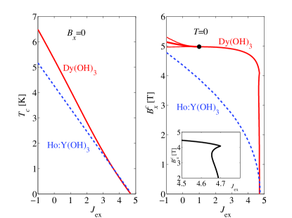
Figure 4: The effect of the value of the exchange constant on the phase boundary, $T_{c}$ vs $J_{\rm ex}$ at $B_{x}$=0 (left) and $B_{x}^{c}$ vs $J_{\rm ex}$ at $T=0$ (right). Solid and dashed lines are used for Dy(OH)₃ and Ho(OH)₃, respectively. The inset of the right graph shows a focus on the features of the high $J_{\rm ex}$ regime in the Dy(OH)₃ plot. The dot in the right panel indicates the tricritical point. The two additional lines at the left side of the tricritical point mark the limits of superheating and supercooling regimes. In the calculations, the CFP of Ref. [Scott, 1970] were used.

IV Effective $S=1/2$ Hamiltonian

In this section we show that Ho(OH)₃ and Tb(OH)₃ can be described with good accuracy by an effective TFIM Hamiltonian. On the other hand, although Dy(OH)₃ has been referred in the literature as an Ising material Catanese and Meissner (1973); Tigges and Wolf (1987), we find that it is not possible to describe the magnetic properties of this material within the framework of an effective Ising Hamiltonian that neglects the effect of the excited crystal field states.

To be able to identify a material as a realization of an effective microscopic Ising model, the following conditions should apply Wolf (2000):

• There has to be a ground state doublet or a close pair of singlets that are separated from the next energy level by an energy gap that is large in comparison with the critical temperature. This ensures that at the temperatures of interest only the two lowest levels are significantly populated.

• To first order, there has to be no transverse susceptibility. It means that there should be no matrix elements of $(J_{x},J_{y})$ operators between the two states of the ground doublet.

• Furthermore, the longitudinal (in the easy axis direction) susceptibility has to be predominantly controlled by the two lowest levels. In other words, there has to be no significant mixing of the states of the lowest doublet with the higher levels via the internal mean field along the Ising direction. In more technical terms, the van Vleck susceptibility should play a negligible role to the non-interacting (free ion) susceptibility near the critical temperature Jensen and Mackintosh (1991).

• In setting up the above conditions, one is in effect requesting that a material be describable as a TFIM from a miscroscopic point of view. However, one can, alternatively, ask whether the quantum critical point of a given material is in the same universality class as the relevant transverse field Ising model. In such a case, as long as transition is second order, then sufficiently close to the quantum critical point, a mapping to an effective TFIM is always in principle possible. However, it can be difficult to estimate the pertinent parameters entering the Ginzburg-Landau-Wilson theory describing the transition. From that perspective, the first and the third point above are always fulfilled sufficiently close to a second order quantum critical point ref .

The first condition is not satisfied in the case of Dy(OH)₃. The energy gap of 7.8 cm^-1 $\approx$ 11.2 K is not much larger than the mean-field critical temperature $T_{c}\sim 5.31\leavevmode\nobreak\ {\rm K}$. Hence, at temperatures close to $T_{c}$, the first excited doublet state is also significantly populated. Furthermore, and most importantly, in the context of a field-induced quantum phase transition, the third condition above is also not satisfied. Hence, even at low temperatures, because of the admixing of the two lowest energy states with the higher energy levels that is induced via the internal (mean) field from the surrounding ions, Dy(OH)₃ cannot by described by an effective microscopic Ising model that solely considers the ground doublet and ignores the excited crystal field states. This effect and the associated role of nonzero $J_{z}$ matrix elements between the ground state and higher crystal field levels is discussed in more detail in Appendix A. As an interesting consequence of this participation of the higher energy levels, we predict that, unlike in the TFIM of Eq. (1), a first order phase transition may occur at high transverse field in Dy(OH)₃ (see Section V.1).

For Ho(OH)₃ and Tb(OH)₃ we construct an effective Ising Hamiltonian, following the method of Refs. [Chakraborty et al., 2004; Tabei et al., 2008a, b]. We diagonalize exactly the noninteracting Hamiltonian, ${\cal H}_{0}$ of Eq. (4), for each value of the transverse field, $B_{x}$. We denote the two lowest states by $\left|\alpha(B_{x})\right\rangle$ and $\left|\beta(B_{x})\right\rangle$ and their energies by $E_{\alpha}(B_{x})$ and $E_{\beta}(B_{x})$, respectively. a transverse field enforces a unique choice of basis, in which the states can be interpreted as $\left|\rightarrow\right\rangle$ and $\left|\leftarrow\right\rangle$ in the Ising subspace. We introduce a new $\left|\uparrow\right\rangle$ and $\left|\downarrow\right\rangle$ basis, in which the $J_{z}$ matrix elements are diagonal, by performing a rotation

$$\begin{array}[]{l}\left|\uparrow\right\rangle=\frac{1}{\sqrt{2}}(\left|\alpha(B_{x})\right\rangle+\exp(i\theta)\left|\beta(B_{x})\right\rangle),\\ \left|\downarrow\right\rangle=\frac{1}{\sqrt{2}}(\left|\alpha(B_{x})\right\rangle-\exp(i\theta)\left|\beta(B_{x})\right\rangle).\end{array}$$ (9)

In this basis, the effective single ion Hamiltonian, describing the two lowest states, is of the form

$$\mathcal{H}_{T}=E_{{\rm CM}}(B_{x})-\frac{1}{2}\Delta(B_{x})\sigma^{x},$$ (10)

where $E_{{\rm CM}}(B_{x})=\frac{1}{2}(E_{\alpha}(B_{x})+E_{\beta}(B_{x}))$ and $\Delta(B_{x})=E_{\beta}(B_{x})-E_{\alpha}(B_{x})$. Thus the splitting of the ground state doublet plays the role of a transverse magnetic field, $\Gamma\equiv\frac{1}{2}\Delta(B_{x})$ in Eq. (1). In the case of Tb(OH)₃, after performing the rotation (9), even at $B_{x}=0$, a small transverse field term ($\Gamma=\frac{1}{2}\Delta(0)>0$) is present in Hamiltonian (10). For Dy(OH)₃ and Ho(OH)₃, the splitting of the energy levels, obtained via exact diagonalization was already discussed at the end of Section II and is shown in Fig. 2. To include the interaction terms in our Ising Hamiltonian, we expand the matrix elements of $J_{x}$, $J_{y}$ and $J_{z}$ operators in terms of the $\sigma^{\nu}$ ($\nu=x,y,z$) Pauli matrices and a unit matrix, $\sigma^{0}\equiv{\openone}$,

$$J_{i,\mu}=C_{\mu}{\openone}+\sum_{\nu=x,y,z}C_{\mu\nu}(B_{x})\sigma_{i}^{\nu}.$$ (11)

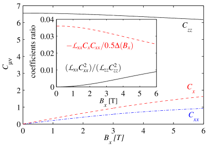
Figure 5: The coefficients in the projection of ${\bm{J}}$ operators onto the two dimensional Ising subspace for Ho(OH)₃. The inset shows the ratios of the coefficients present in Eq. (12).

By replacing all $J_{i,{\mu}}$ operators in the interaction term of Hamiltonian (5) by the two dimensional representation of Eq. (11), one obtains in general a lengthy Hamiltonian containing all possible combinations of spin-$\frac{1}{2}$ interactions. In the present case, the resulting Hamiltonian is considerably simplified by the crystal symmetries and the consequential vanishing of off-diagonal elements of the interaction matrix $\mathcal{L}_{\mu\nu}$. This would not be the case for diluted Ho_xY_1-xF₄ (see Ref. [Tabei et al., 2008b]]). After performing the transformation in Eq. (9), we have $J_{i}^{z}=C_{zz}\sigma_{i}^{z}$, $J_{i}^{y}=C_{yy}\sigma_{i}^{y}$ and $J_{i}^{x}=C_{xx}\sigma_{i}^{x}+C_{x}{\openone}$. Hence, we can rewrite the mean-field Hamiltonian (7) in the form

$$\mathcal{H}_{\rm MF} = (\mathcal{L}_{zz}+z{\cal J}_{\rm ex})C_{zz}^{2}m_{z}\sigma^{z}+\left(\mathcal{L}_{xx}C_{x}C_{xx}-\frac{1}{2}\Delta(B_{x})\right)\sigma^{x}$$ (12)

$$+ (\mathcal{L}_{xx}+z{\cal J}_{\rm ex})C_{xx}^{2}m_{x}\sigma^{x}+(\mathcal{L}_{yy}+z{\cal J}_{\rm ex})C_{yy}^{2}m_{y}\sigma^{y},$$

where $m_{\nu}\equiv\left\langle\sigma^{\nu}\right\rangle$ and $\left\langle\ldots\right\rangle$ denotes a Boltzmann thermal average.

The $C_{zz}$, $C_{xx}$ and $C_{x}$ coefficients for Ho(OH)₃ are plotted in Fig. 5. The inset shows a comparison of the terms in $\mathcal{H}_{\rm MF}$. In Ho(OH)₃, the coefficient ${\it\mathcal{L}_{xx}}{\it C_{xx}}^{2}$ (the fourth therm of $\mathcal{H}_{\rm MF}$) does not exceed 1.5% of the effective transverse field, $\Gamma={\it\mathcal{L}_{xx}}{\it C_{x}}{\it C_{xx}}-\frac{1}{2}\Delta(B_{x})$. In Tb(OH)₃, this ratio is even smaller, and we thus neglect it, further motivated by the fact that doing so decouples $m_{z}$ from $m_{x}$ and make the problem simpler. The term $\mathcal{L}_{yy}{C_{yy}}^{2}m_{y}\sigma^{y}$ in Eq. 12 can be omitted, since due to symmetry $m_{y}\equiv\langle\sigma^{y}\rangle=0$. The interaction correction, ${\it\mathcal{L}_{xx}}{\it C_{x}}{\it C_{xx}}$, to the effective transverse field, $\Gamma$, is of order of 3% of $\Gamma$ and we retain it in our calculations. Thus, we finally write

$$\mathcal{H}_{\rm MF}=P\sigma^{z}+\Gamma\sigma^{x},$$ (13)

where $P={\it\mathcal{L}_{zz}}{\it C_{zz}}^{2}m_{z}$ and $\Gamma={\it\mathcal{L}_{xx}}{\it C_{x}}{\it C_{xx}}-\frac{1}{2}\Delta(B_{x})$.

Diagonalizing the Hamiltonian (13) allows us to evaluate $m_{z}$ and $m_{x}\equiv\langle\sigma^{x}\rangle$, giving well known formulae Chakrabarti et al. (1996):

$$\begin{array}[]{c}m_{x}=\frac{\Gamma}{\sqrt{P^{2}+\Gamma^{2}}}\tanh(\sqrt{P^{2}+\Gamma^{2}}/T),\\ m_{z}=\frac{P}{\sqrt{P^{2}+\Gamma^{2}}}\tanh(\sqrt{P^{2}+\Gamma^{2}}/T)\end{array},$$ (14)

and the phase boundary,

$$T_{c}(B_{x})=\frac{\Gamma(B_{x})}{{\rm atanh}(\frac{\Gamma(B_{x})}{\mathcal{L}_{zz}C_{zz}^{2}})}.$$ (15)

In Fig. 6, we show that Eq. (15) yields a phase diagram that only insignificantly differs from the one obtained from the full diagonalization of ${\cal H}_{\rm MF}$ in Eq. (7) shown in Fig. 3, in the case of Ho(OH)₃, and, in the case of Tb(OH)₃, the discrepancy is even smaller because the energy gap to the third crystal field state, 118 cm${}^{-1}\simeq$ 170 K, is very large compared to $T_{c}^{\rm MF}=5.59$ K.

As alluded to above, in the case of Dy(OH)₃, a description in terms of an effective Ising Hamiltonian method does not work because of the admixing between states of the two lowest doublets induced by the local mean-field that is proportional to $\left\langle J_{z}\right\rangle$ (see Appendix A). The dashed line in the last panel of Fig. 6 shows the incorrect phase diagram obtained for Dy(OH)₃ obtained using an effective spin-$1/2$ Hamiltonian constructred from only the ground doublet. It turns out that a form of the method of Section IV can still be used. However, instead of keeping only two levels in the interaction Hamiltonian, one needs to retain at least four states. In analogy with the procedure in Section IV, we diagonalize the single ion Hamiltonian ${\cal H}_{0}$ of Eq. (4) which consist of the crystal field Hamiltonian and the transverse field term. Next, we write an effective interaction Hamiltonian using the four (or six) lowest eigenstates of ${\cal H}_{0}$. The resulting effective Hamiltonian is then used in the self-consistent Eqs. (8). For example, for $B_{x}=4.8$ T, proceeding by keeping only the four lowest eigenstates of ${\cal H}_{0}$ to construct the effective Hamiltonian, one finds a critical temperature that is only about 3% off compared to a calculation that keeps all 16 eigentates of ${\cal H}_{0}$. This difference drops below 1% when keeping the 6 lowest eigenstates of ${\cal H}_{0}$.

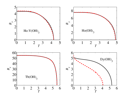
Figure 6: Comparison of the phase diagrams obtained with diagonalization of the full manifold (black, solid lines) and with effective spin-1/2 Hamiltonian (red, dashed lines). Calculation for Ho(OH)₃ were performed using the CFP of Karmakar et al. Karmakar et al. (1981, 1982).

Having explored the quantitative validity of the spin-1/2 TFIM description of Ho(OH)₃ and Tb(OH)₃ in nonzero $B_{x}$, we now turn to the problem of the first order PM to FM transition at large $B_{x}$ and low temperature in Dy(OH)₃, exposed in the numerical solution of the self-consistent equations comprised in Eq. (8) (with $\mu=x,z$).

V First order transition

The first order transition in Dy(OH)₃ takes its origin in the sizeable admixing among the four lowest levels induced by the the local mean-field that is proportional to $\left\langle J_{z}\right\rangle$. Under the right temperature and field conditions, two free-energy equivalent configurations can exist: an ordered state with some not infinitesimally small magnetization, $\left\langle J_{z}\right\rangle>0$, and a state with zero magnetic moment, $\left\langle J_{z}\right\rangle=0$. To simplify the argument, we consider how this occurs at $T=0$. At first, let us look at the situation when the longitudinal internal mean field induces an admixing of the ground state with the first excited state only (as in the TFIM). In such a case, there is only a quadratic dependence of the ground state energy on the longitudinal mean field, $B_{z}^{\rm MF}$, and, consequently, only one energy minimum is possible. Now, if there is an admixing of the ground state and at least three higher levels, the dependency of the ground state energy on $B_{z}^{{\rm MF}}$ is of fourth order and two energy minima are, in principle, possible. Thus, at a certain value of external parameters the system can acquire two energetically equivalent states, one with zero and the other with a non-zero magnetization. When passing through this point, either by varying the transverse field or the temperature, a first order phase transition characterized by a magnetization discontinuity occurs. To make this discussion more formal, we now proceed with a construction of the Ginzburg-Landau theory for Dy(OH)₃ for arbitrary $B_{x}$ in the regime of $B_{x}$ and $T$ values where the paramagnetic to ferromagnetic transition is second order. This allows us to determine the the tricritical transverse field value above which the transition becomes first order.

V.1 Ginzburg-Landau Theory

To locate the tricritical point for Dy(OH)₃, we perform a Landau expansion of the mean-field free energy, ${\cal F}_{\rm MF}(\left\langle J_{x}\right\rangle,\left\langle J_{z}\right\rangle)$. Next, we minimize ${\cal F}_{\rm MF}$ with respect to $\left\langle J_{x}\right\rangle$, leaving $\left\langle J_{z}\right\rangle$ as the only free parameter. The mean-field free energy can be written in the form

$$\mathcal{F}_{\rm MF}\left(\left\langle J_{x}\right\rangle,\left\langle J_{z}\right\rangle\right) = -T\log Z\left(\left\langle J_{x}\right\rangle,\left\langle J_{z}\right\rangle\right)$$ (16)

$$- \frac{1}{2}\left(\mathcal{L}_{xx}\left\langle J_{x}\right\rangle^{2}+\mathcal{L}_{zz}\left\langle J_{z}\right\rangle^{2}\right),$$

where $Z\left(\left\langle J_{x}\right\rangle,\left\langle J_{z}\right\rangle\right)$ is the partition function.

Just below the transition, in the part of the phase diagram where the transition is second order, $\left\langle J_{z}\right\rangle$ is a small parameter (i.e. has a small dimensionless numerical value). We therefore make an expansion for $\left\langle J_{x}\right\rangle$ as a function of $\left\langle J_{z}\right\rangle$, which we write it in the form:

$$\left\langle J_{x}\right\rangle=\left\langle J_{x}\right\rangle_{0}+\delta({\left\langle J_{z}\right\rangle}).$$ (17)

$\left\langle J_{x}\right\rangle_{0}$ is the value of $\left\langle J_{x}\right\rangle$ that extremizes ${\cal F}_{\rm MF}$ when $\left\langle J_{z}\right\rangle=0$. $\delta({\langle J_{z}\rangle})$ is a perturbatively small function of $\left\langle J_{z}\right\rangle$, which we henceforth simply denote $\delta$, and which is our series expansion small parameter for $\langle J_{x}\rangle$. Substituting expression (17) to $\mathcal{H}_{\rm MF}$ of Eq. (7), and setting $J_{\rm ex}=0$ for the time being, we have

$$\mathcal{H} = {\cal H}_{\rm cf}({\bm{J}}_{i})-g\mu_{\rm B}B_{x}J_{x}$$ (18)

$$+ \mathcal{L}_{xx}J_{x}(\left\langle J_{x}\right\rangle_{0}+\delta)+\mathcal{L}_{zz}J_{z}\left\langle J_{z}\right\rangle,$$

or

$$\mathcal{H}=\mathcal{H}_{0}(B_{x},\left\langle J_{x}\right\rangle_{0})+\mathcal{L}_{xx}J_{x}\delta+\mathcal{L}_{zz}J_{z}\left\langle J_{z}\right\rangle,$$ (19)

where for brevity, as in Eq. (7), the constant term has been dropped because, again, it does not affect the expectation values needed for the calculation.

The power series expansion of the partition function, and then of the free energy (16), can be calculated from the eigenvalues of Hamiltonian (19). Instead of applying standard quantum-mechanical perturbation methods to Eq. (19), we obtain the expansion of energy levels as a perturbative, ‘seminumerical’, solution to the characteristic polynomial equation

$$\det\left[\mathcal{H}_{0}+\mathcal{L}_{xx}J_{x}\delta+\mathcal{L}_{zz}J_{z}\left\langle J_{z}\right\rangle-E_{n}\right]=0.$$ (20)

We can easily implement this procedure by using a computer algebra method (e.g. Maple$\texttrademark$ or Mathematica$\texttrademark$). To proceed, we substitute a formal power series expansion of the solution

$$E_{n}=E_{n}^{(0,0)}+E_{n}^{(0,1)}\delta+E_{n}^{(2,0)}\left\langle J_{z}\right\rangle^{2}+E_{n}^{(2,1)}\left\langle J_{z}\right\rangle^{2}\delta+\ldots,$$ (21)

to Eq. (20), containing all the terms of the form $E_{n}^{(\alpha,\beta)}\left\langle J_{z}\right\rangle^{\alpha}\delta^{\beta}$, where $\alpha+2\beta\leq 6$, as will be justified below Eq. (24). To impose consistency of the resulting equation obtained from Eq. (20) and Eq. (21), up to sixth order of the expansion in $\left\langle J_{z}\right\rangle$ in), we need to equate to zero all the coefficient with the required order of $\left\langle J_{z}\right\rangle$ and $\delta$, i.e. $\alpha+2\beta\leq 6$. This gives a system of equations that can be numerically solved for the coefficients $E_{n}^{(k,l)}$, where $k,l>0$. By $E_{n}^{(0,0)}$ we denote the eigenvalues of the Hamiltonian $\mathcal{H}_{0}(B_{x},\left\langle J_{x}\right\rangle_{0})$.

We use the perturbed energies, $E_{n}$, of Eq. (21) to calculate the partition function

$$Z(\delta,\left\langle J_{z}\right\rangle)=\sum_{n}e^{-E_{n}/T}$$ (22)

and substitute it in Eq. (16). We Taylor expand the resulting expression to obtain the numerical values of the expansion coefficients in the form

$${\cal F}_{\rm MF}=A^{(0,0)}+A^{(2,0)}\left\langle J_{z}\right\rangle^{2}+A^{(0,1)}\delta+A^{(2,1)}\left\langle J_{z}\right\rangle^{2}\delta+\ldots.$$ (23)

The free energy ${\cal F}_{\rm MF}$ is a symmetric function of $\left\langle J_{z}\right\rangle$, so the expansion (23) contains only even powers of $\left\langle J_{z}\right\rangle$. We minimize ${\cal F}_{\rm MF}$ in Eq. (23) with respect to $\delta$. To achieve this, we have to solve a high order polynomial equation $d{\cal F}_{\rm MF}/d\delta=0$. Again, we do it by substituting to the equation a formal power series solution

$$\delta({\langle J_{z}\rangle})=D_{2}\left\langle J_{z}\right\rangle^{2}+D_{4}\left\langle J_{z}\right\rangle^{4}+\ldots$$ (24)

and then solve it for the values of the expansion parameters $D_{n}$. Due to symmetry, only even powers of $\left\langle J_{z}\right\rangle$ are present and, from the definition of $\delta$, the constant $\langle J_{z}\rangle$-independent term is equal to zero. From the form of the expansion in Eq. (24), we see that to finally obtain the free energy expansion in powers of $\left\langle J_{z}\right\rangle$, up to $n$-th order, we need to consider only the terms $\left\langle J_{z}\right\rangle^{\alpha}\delta^{\beta}$ where $\alpha+2\beta\leq n$. Finally, by substituting $\delta$ from Eq. (24) into Eq. (23), we obtain the power series expansion of the free energy in the form:

$${\cal F}_{\rm MF}=C_{0}+C_{2}\left\langle J_{z}\right\rangle^{2}+C_{4}\left\langle J_{z}\right\rangle^{4}+C_{6}\left\langle J_{z}\right\rangle^{6}.$$ (25)

In the second order transition region, the condition $C_{2}=0$ with $C_{4}>0$ parametrizes the phase boundary. The equations $C_{2}=C_{4}=0$ gives the condition for the location of the tricritical point. In the regime where $C_{4}<0$, the condition $C_{2}=0$ gives the supercooling limit. The first order phase transition boundary is located where the free energy has the same value at both local minima. Increasing the value of the control parameters, $T$ and $B_{x}$, above the critical value, until the second (nontrivial) local minimum of ${\cal F}_{\rm MF}$ vanishes, gives the superheating limit.

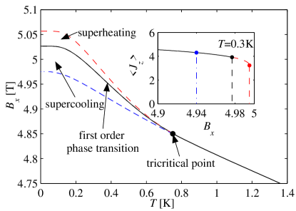
Figure 7: Tricritical behavior of Dy(OH)₃. The continuous line marks the phase boundary. The dot indicates the location of the tricritical point. The upper and lower lines (dashed) are the limits of the superheating and supercooling regimes, respectively. As an example, the inset shows the order parameter $\left\langle J_{z}\right\rangle$ vs $B_{x}$, at the temperature $T=$0.3 K. For this temperature, the phase transition occurs at $B_{x}\approx 4.98$ T. The upper dashed extension of the solid line corresponds to the superheating limit. The dash-dotted line to the left of the tricritical point shows the transition at the supercooling limit.

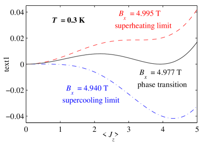
Figure 8: Free energy vs average magnetic moment $\left\langle J_{z}\right\rangle$ at the temperature of 0.3 K. The free energy at the first order phase transition is plotted with continuous line. The upper (dashed) line shows the free energy at the boundary of the superheating limit. The lower (dot-dashed) line shows the free energy when the system passes through the supercooling limit. All the plots show the free energy displaced by a constant chosen such that their shape can be compared.

The location of the tricritical point is $T_{c}^{\rm TCP}=$0.75 K, $B_{x}^{\rm TCP}=$4.85 T. We show in Fig. 7 the first and the second order transition phase boundary; the tricritical point is marked with a dot. In the first order transition regime, the superheating and supercooling limits are also plotted. $\langle J_{z}\rangle$ ceases to be a small parameter for values of $T$ and $B_{x}$ ‘away’ from the tricritical point. Thus, the two upper curves in the phase diagram of Fig. 7 are determined from a numerical search for both local minima of the exact mean-field free energy in Eq. (16) without relying on a small $\left\langle J_{z}\right\rangle$ and $\delta(\left\langle J_{z}\right\rangle)$ expansion. The supercooling limit is calculated from the series expansion (25) and determined by the condition $C_{2}=0$.

In the inset of Fig. 7, we show the average magnetic moment, $\left\langle J_{z}\right\rangle$, as a function of the transverse field, at the temperature of 0.3 K. The dots and the dashed lines mark the supercooling limit, first order phase boundary and the superheating limit, in order of increasing $B_{x}$. The shape of the free energy at these three characteristic values of the magnetic field, $B_{x}$, at temperature of 0.3 K, is shown in Fig. 8.

In Fig. 8, we plot the free energy as a function of $\left\langle J_{z}\right\rangle$, where $\left\langle J_{x}\right\rangle$ is minimizing ${\cal F}_{\rm MF}$ as a function of $\left\langle J_{z}\right\rangle$ at $T=0.3$ K. Free energy at the phase transition ($B_{x}\approx$ 4.977 T) is plotted with a continuous line. The dashed and dot-dashed plots show free energy at the superheating and supercooling limits, at $B_{x}\approx$ 4.995 T and $B_{x}\approx$ 4.940 T, respectively. The free energy clearly shows the characteristic structure (e.g. barrier) of a system with a first order transition. It would be interesting to investigate whether the real Dy(OH)₃ material exhibits such a $B_{x}-$induced first order PM to FM transition at strong $B_{x}$. In the event that the transition is second order down to $T=0$ and $B_{x}=B_{x}^{c}$, Dy(OH)₃ would offer itself as another material to investigate transverse field induced quantum criticality (see 4^th item in the list at the beginning of Section IV). However, a quantitative microscopic description at strong $B_{x}$ would nevertheless require that the contribution of the lowest pairs of excited crystal field states be taken into account.

One may be tempted to relate the existence of a first order transition in Dy(OH)₃, on the basis of Eq. (23), with two expansion parameters $\langle J_{z}\rangle$ and $\delta$, to the familiar problem where a free-energy function, ${\cal F}(m,\epsilon)$, of two order parameters $m$ and $\epsilon$,

$${\cal F}(m,\epsilon) = \frac{a}{2}m^{2}+\frac{|b|}{4}m^{4}+\frac{|c|}{6}m^{6}+\frac{K}{2}\epsilon^{2}-g\epsilon m^{2}$$

displays a first order transition when $g^{2}/K>b/2$. However, we have found that this analogy is not useful and the mechamism for the first order transition is not trivially due to the presence of two expansion parameters, $\left\langle J_{z}\right\rangle$ and $\delta$, in the expansion (23). It is rather the complex specific details of the crystal field Hamiltonian for Dy(OH)₃ that are responsible for the first order transition. For example, at a qualitative level, a first order transition still occurs even if $\delta(\left\langle J_{z}\right\rangle)$, in Eq. (17), is taken to be 0, for all values of $\left\langle J_{z}\right\rangle$.

V.2 The effect of longitudinal magnetic field and exchange interaction on the existence of first order transition in Dy(OH)₃

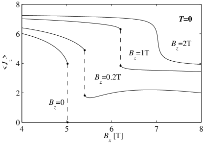
Figure 9: Average magnetic moment, $\left\langle J_{z}\right\rangle$, vs transverse magnetic field, $B_{x}$, at $T=0$, $J_{\rm ex}=0$, for different values of longitudinal magnetic field, $B_{z}$.

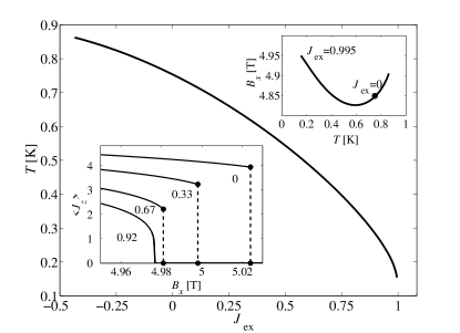
Figure 10: Temperature corresponding to the TCP as a function of nearest-neighbor exchange constant $J_{\rm ex}$. The upper inset shows position of the TCP in the phase diagram plane for the same range of exchange constant as in the main plot. For an exchange $J_{\rm ex}>J_{\rm ex}^{\rm 2nd}$, with $J_{\rm ex}^{\rm 2nd}=0.995$, the tricritical point at $T>0$ ceases to exist. The lower inset shows average magnetic moment $\left\langle J_{z}\right\rangle$ vs transverse field $B_{x}$ at temperature $T=$0, for the shown values of exchange constant $J_{\rm ex}$.

Having found that the PM to FM transition may be first order in Dy(OH)₃ at large $B_{x}$ (low $T$), it is of interest to investigate briefly two effects of physical relevance on the predicted first order transition. Firstly, since the transition is first order from $0\leq T\leq T^{\rm TCP}$, one may ask what is the critical longitudinal field, $B_{z}$, required to push the tricritical point from finite temperature down to zero temperature. Focusing on the CFP of Scott et al. from Refs. [Scott, 1970; Scott and Wolf, 1969; Kahle et al., 1986; Scott et al., 1969], we find that a sufficiently strong magnetic field, $B_{z}$, applied along the longitudinal $z$ direction destroys the first order transition, giving rise to an end critical point. We plot in Fig. 9 the magnetization, $\left\langle J_{z}\right\rangle$, as a function of $B_{x}$ for different values of $B_{z}$ at $T=0$. We see that a critical value of $B_{z}$ is reached between 1 T and 2 T, where the first order transition disappears, giving rise to an end critical point at $T=0$. Hence, assuming that the low-temperature $B_{x}$-driven PM to FM transition is indeed first order in Dy(OH)₃, the results of Fig. (9) indicate that the critical longitudinal field for a quantum critical end point is easily accessible, using a so-called vector magnet (i.e. with tunable horizontal, $B_{x}$, and vertical, $B_{z}$, magnetic fields) K. Deguchi and Maeno (2004).

It was discussed in Section III (Fig. 4) that the (yet undetermined) nearest-neighbor exchange interaction, $J_{{\rm ex}}$, affects the zero $B_{x}$ critical temperature, $T_{c}$, and the zero temperature critical transverse field, $B_{x}^{c}$. It is also of interest to explore what is the role of $J_{{\rm ex}}$ on the location (temperature and transverse field) of the tricritical point in Dy(OH)₃.

We plot in Fig. 10 the temperature corresponding to the tricritical point (TCP) as a function of antiferromagnetic exchange and, in the upper inset, the location of the TCP on the phase diagram is presented. The location of the TCP was calculated using the semi-analytical expansion described in Section V.1. We found that the system ceases to exhibit a first order transition at nonzero temperature when the value of nearest neighbor exchange constant, $J_{{\rm ex}}$, exceeds $J_{\rm ex}^{\rm 2nd}=0.995$. At $B_{x}$=0, the critical temperature calculated with the value of exchange constant $J_{{\rm ex}}$=0.995 is 4.09 K. In the lower inset of Fig. 10 we plot the average magnetic moment, $\left\langle J_{z}\right\rangle$, as a function of $B_{x}$ at zero temperature, for different values of $J_{\rm ex}$. The top inset shows a parametric plot of the position of the TCP in the $(T,B_{x})$ plane as $J_{\rm ex}$ is varied.

VI Conclusion

We have presented a simple mean-field theory aimed at motivating an experimental study of transverse-field-induced phase transitions in the insulating rare-earth Ising RE(OH)₃ (RE=Dy, Ho) uniaxial dipolar ferromagnetic materials.

In setting out to perform the above calculations, we were mostly motivated in identifying a new class of materials as analogous as possible to LiHo_xY_1-xF₄, where interesting phenomena, both in zero and nonzero applied transverse field $B_{x},$ have been observed. In particular, we were interested in finding compounds where a systematic comparison between a non-Kramers (e.g. Ho³⁺) and a Kramers (e.g. Dy³⁺) variant could be investigated. From our study, we are led to suggest that an experimental study of the Dy_xY_1-x(OH)₃ and Ho_xY_1-x(OH)₃ materials could bring new pieces of information on the physics that may be at play in LiHo_xY_1-xF₄ and to ascertain if that physics is unique to LiHo_xY_1-xF₄ or if it also arises in other diluted dipolar Ising ferromagnets.

Depending on the details of the Hamiltonian characterizing Dy(OH)₃, it may be that a first order transition occurs at low temperature (large $B_{x}$), due to the admixing between the ground doublet and the low-lying crystal field states that is induced by the spin-spin interactions. For the same reason, we find that Dy(OH)₃ is not well described by an effective microscopic transverse field Ising model (TFIM). On the other hand, Ho(OH)₃ appears to be very well characterized by a TFIM and, therefore, constitutes a highly analogous variant of LiHoF₄. Tb(OH)₃ is also very well described by a TFIM. Unfortunately, in that case, the critical $B_{x}$, $B_{x}^{c}$, appears prohibitively large to be accessed via in-house commercial magnets.

We hope that our work will stimulate future systematic experimental investigations of these materials and, possibly, help shed some light on the rather interesting problems that pertain to the fundamental nature of classical and quantum critical phenomena in disordered dipolar systems and which have been raised by nearly twenty years of study of LiHo_xY_1-xF₄.

Appendix A Perturbative calculation of the phase diagram in Dy(OH)₃

To investigate the role of the $J_{z}$ matrix elements between the two lowest states and the first excited levels on the magnetic behavior of Dy(OH)₃, we calculate the critical temperature for a second order transition using second order perturbation theory. This method is exact in the second order phase transition regime, where $B_{x}$ is less than the tricritical field value, $B_{x}^{\rm TCP}$ ($B_{x}^{\rm TCP}=4.85\leavevmode\nobreak\ {\rm T}$ when using the CFP of Scott et al.).

For a given value of the transverse field, $B_{x}$, and the corresponding value of average magnetization in transverse direction, $\left\langle J_{x}\right\rangle$, we consider $\mathcal{L}_{zz}J_{z}\left\langle J_{z}\right\rangle$ term as a perturbation to the reference mean-field Hamiltonian,

$$\mathcal{H}_{0}={\cal H}_{\rm cf}(\bm{J}_{i})-g\mu_{\rm B}B_{x}J_{x}+\mathcal{L}_{xx}J_{x}\left\langle J_{x}\right\rangle,$$ (26)

describing the PM phase at a temperature $T>T_{c}(B_{x})$ as in Eq. 7 Here too, we have dropped the constant terms. The eigenvalues, $E_{p}$, and eigenstates, $\left|p\right\rangle$, of the perturbed Hamiltonian,

$$\mathcal{H}=\mathcal{H}_{0}+\mathcal{L}_{zz}J_{z}\left\langle J_{z}\right\rangle,$$ (27)

are written in terms of eigenvalues, $E_{p}^{(0)}$, and eigenstates, $\left|p^{(0)}\right\rangle$, of the unperturbed Hamiltonian, $\mathcal{H}_{0}$, of Eq. (26),

$$E_{p}=E_{p}^{(0)}+\left\langle J_{z}\right\rangle E_{p}^{(1)}+\left\langle J_{z}\right\rangle^{2}E_{p}^{(2)},$$ (28)

$$|p\rangle=|{p^{(0)}}\rangle+\left\langle J_{z}\right\rangle\sum_{k\neq p}c_{p,k}^{(1)}|{k^{(0)}}\rangle.$$ (29)

The coefficients of the perturbative expansion are given by

$$E_{p}^{(1)}=\mathcal{L}_{zz}J_{pp}^{z},$$ (30)

$$E_{p}^{(2)}=\sum_{k\neq p}\frac{\mathcal{L}_{zz}^{2}|J_{kp}^{z}|^{2}}{E_{p}^{(0)}-E_{k}^{(0)}}$$ (31)

and

$$c_{pk}^{(1)}=\frac{\mathcal{L}_{zz}J_{kp}^{z}}{E_{p}^{(0)}-E_{k}^{(0)}},$$ (32)

where $J_{kp}^{z}=\left\langle k^{(0)}\right|J_{z}\left|p^{(0)}\right\rangle$ are the matrix elements of the $J_{z}$ operator in the basis of eigenvectors of the unperturbed Hamiltonian, $\mathcal{H}_{0}$. The applied magnetic field, $B_{x}$, lifts the degeneracy of the Kramers doublets, thus we can use the nondegenerate perturbation method. The diagonal elements of the $J_{z}$ operator vanish, hence, the first order correction to energy vanish, $E_{p}^{(1)}=J_{pp}^{z}=0$.

We calculate the thermal average of the $J_{z}$ operator,

$$\left\langle J_{z}\right\rangle=\sum_{p}\left\langle p\right|J_{z}\left|p\right\rangle e^{-E_{p}/T}/Z,$$ (33)

using the perturbed eigenstates, $\left|p\right\rangle$, and eigenvalues, $E_{p}$, and where $Z=\sum_{p}e^{-E_{p}/T}.$ Keeping only terms up to third order in $\left\langle J_{z}\right\rangle$ in the expansion of Eq. (33), we find

$$\frac{1}{Z}e^{-E_{p}/T}=n_{p}^{(0)}\left(1+K_{p}\left\langle J_{z}\right\rangle^{2}\right)$$ (34)

and

$$\left\langle p\right|J_{z}\left|p\right\rangle=2\mathcal{L}_{zz}\left\langle J_{z}\right\rangle\sum_{k\neq p}\frac{|J_{pk}^{z}|^{2}}{E_{p}^{(0)}-E_{k}^{(0)}},$$ (35)

where, for convenience, we write $n_{p}^{(0)}=e^{-E_{p}^{(0)}/T}/Z^{(0)}$, $Z^{(0)}=\sum_{p}e^{-E_{p}^{(0)}/T}$ and $K_{p}=\frac{1}{T}\left(\sum_{k}n_{k}^{(0)}E_{k}^{(2)}-E_{p}^{(2)}\right)$. Thus, we can write

$$\left\langle J_{z}\right\rangle=2\left\langle J_{z}\right\rangle\sum_{p}n_{p}^{(0)}\left(1+K_{p}\left\langle J_{z}\right\rangle^{2}\right)\sum_{k\neq p}\frac{\mathcal{L}_{zz}|J_{pk}^{z}|^{2}}{E_{p}^{(0)}-E_{k}^{(0)}},$$ (36)

and finally, we get

$$\left\langle J_{z}\right\rangle^{2}=\frac{1-2\sum_{p,k\neq p}n_{p}^{(0)}\frac{\mathcal{L}_{zz}|J_{pk}^{z}|^{2}}{E_{p}^{(0)}-E_{k}^{(0)}}}{2{\sum}_{p,k\neq p}n_{p}^{(0)}K_{p}\frac{\mathcal{L}_{zz}|J_{pk}^{z}|^{2}}{E_{p}^{(0)}-E_{k}^{(0)}}}.$$ (37)

Putting $\left\langle J_{z}\right\rangle=0$ in Eq. (37) we obtain the condition for the critical temperature $T_{c}$:

$$2\sum_{p,k\neq p}\frac{\mathcal{L}_{zz}|J_{pk}^{z}|^{2}}{E_{p}^{(0)}-E_{k}^{(0)}}e^{\frac{-E_{p}^{(0)}}{T_{c}}}=1.$$ (38)

In solving Eq. (38) for $T_{c}$, we have to self-consistently update the value of $\left\langle J_{x}\right\rangle$ in order to diagonalize $\mathcal{H}_{0}$ in Eq. (26) and to find $E_{p}^{(0)}$. Solving Eq. (38) with only the 4 lowest energy eigenstates (after diagonalizing the full transverse field Hamiltonian of Eq. (4)), yields a phase diagram that is in good agreement for $B_{x}<B_{x}^{\rm TCP}$ with the phase boundary obtained with all crystal field eigenstates (or equivalently from Eq. (8)).

Estimating the values of the elements of the sum in Eq. (38), one can see that the matrix elements of the $J_{z}$ operator, mixing the two lowest states with the excited states, may bring a substantial correction to the value of the critical temperature obtained when only the two lowest eigenstates are considered. In the low temperature regime, one could omit the matrix elements between the states of the excited doublet, but we have to keep the matrix elements between the states of the ground doublet and first excited doublet. The contribution from the further exited states is quite small because of the increasing value of the energy gap present in the denominator in Eq. (38).

At $T$=0, Eq. (35) leads to the equation for the critical transverse field, $B_{x}^{c}$:

$$2\sum_{k\neq 1}\frac{\mathcal{L}_{zz}|J_{1k}^{z}(B_{x}^{c})|^{2}}{E_{1}^{(0)}(B_{x}^{c})-E_{k}^{(0)}(B_{x}^{c})}=1.$$ (39)

Again, we see that the matrix elements of $J^{z}$ operator, admixing the ground state with excited levels, have to be considered. Note that since Eq. (39) pertains to the case of zero temperature, this equation is only valid in a regime where the transition is second order (i.e. when $J_{{\rm ex}}>J_{{\rm ex}}^{\rm 2nd}$).

References

- Sondhi et al. (1997) S. L. Sondhi, S. M. Girvin, J. P. Carini, and D. Shahar, Rev. Mod. Phys. 69, 315 (1997).
- Sachdev (1999) S. Sachdev, Quantum Phase Transitions (Cambridge University Press, Cambridge, 1999).
- Elliott et al. (1970) R. J. Elliott, P. Pfeuty, and C. Wood, Phys. Rev. Lett. 25, 443 (1970).
- Chakrabarti et al. (1996) B. K. Chakrabarti, A. Dutta, and P. Sen, Quantum Ising Phases and Transitions in Transverse Ising Models (Spinger-Verlag, Heidelberg, 1996).
- de Gennes (1963) P. G. de Gennes, Solid State Commun. 1, 132 (1963).
- Chakraborty et al. (2004) P. B. Chakraborty, P. Henelius, H. Kjonsberg, A. W. Sandvik, and S. M. Girvin, Phys. Rev. B 70, 144411 (2004).
- Tabei et al. (2008a) S. M. A. Tabei, M. J. P. Gingras, Y.-J. Kao, and T. Yavors’kii, cond-mat/0801.0443 (2008a).
- Tabei et al. (2008b) S. M. A. Tabei, F. Vernay, and M. J. P. Gingras, Phys. Rev. B 77, 014432 (2008b).
- Binder and Young (1986) K. Binder and A. P. Young, Rev. Mod. Phys. 58, 801 (1986).
- Mydosh (1993) J. A. Mydosh, Spin Glasses: an Experimental Introduction (Taylor & Francis, London, 1993).
- Rieger and Young (1994) H. Rieger and A. P. Young, Phys. Rev. Lett. 72, 4141 (1994).
- Rieger and Young (1996) H. Rieger and A. P. Young, Phys. Rev. B 54, 3328 (1996).
- Guo et al. (1996) M. Guo, R. N. Bhatt, and D. A. Huse, Phys. Rev. B 54, 3336 (1996).
- Griffiths (1969) R. B. Griffiths, Phys. Rev. Lett. 23, 17 (1969).
- McCoy (1969) B. M. McCoy, Phys. Rev. Lett. 23, 383 (1969).
- Reich et al. (1990) D. H. Reich, B. Ellman, J. Yang, T. F. Rosenbaum, G. Aeppli, and D. P. Belanger, Phys. Rev. B 42, 4631 (1990).
- Wu et al. (1991) W. Wu, B. Ellman, T. F. Rosenbaum, G. Aeppli, and D. H. Reich, Phys. Rev. Lett. 67, 2076 (1991).
- Wu et al. (1993) W. Wu, D. Bitko, T. F. Rosenbaum, and G. Aeppli, Phys. Rev. Lett. 71, 1919 (1993).
- Wu (1992) W. Wu, PhD thesis, U. of Chicago (1992).
- Bitko et al. (1996) D. Bitko, T. F. Rosenbaum, and G. Aeppli, Phys. Rev. Lett. 77, 940 (1996).
- Brooke et al. (1999) J. Brooke, D. Bitko, T. F. Rosenbaum, and G. Aeppli, Science 284, 779 (1999).
- Brooke (2000) J. Brooke, Ph.D. thesis, U. of Chicago (2000).
- Ghosh et al. (2002) S. Ghosh, R. Parthasarathy, T. F. Rosenbaum, and G. Aeppli, Science 296, 2195 (2002).
- Ghosh et al. (2003) S. Ghosh, T. F. Rosenbaum, G. Aeppli, and S. N. Coppersmith, Nature 425, 48 (2003).
- Ronnow et al. (2005) H. M. Ronnow, R. Parthasarathy, J. Jensen, G. Aeppli, T. F. Rosenbaum, and D. F. McMorrow, Science 308, 389 (2005).
- Ronnow et al. (2007) H. M. Ronnow, J. Jensen, R. Parthasarathy, G. Aeppli, T. F. Rosenbaum, D. F. McMorrow, and C. Kraemer, Phys. Rev. B 75, 054426 (2007).
- Silevitch et al. (2007a) D. M. Silevitch, D. Bitko, J. Brooke, S. Ghosh, G. Aeppli, and T. F. Rosenbaum, Nature 448, 567 (2007a).
- Silevitch et al. (2007b) D. M. Silevitch, C. M. S. Gannarelli, A. J. Fisher, G. Aeppli, and T. F. Rosenbaum, Phys. Rev. Lett 99, 057203 (2007b).
- Jönsson et al. (2007) P. E. Jönsson, R. Mathieu, W. Wernsdorfer, A. M. Tkachuk, and B. Barbara, Phys. Rev. Lett 98, 256403 (2007).
- C. Ancona-Torres and Rosenbaum (2008) G. A. C. Ancona-Torres, D. M. Silevitch and T. F. Rosenbaum, cond-mat/0801.2335 (2008).
- Jönsson et al. (2008) P. E. Jönsson, R. Mathieu, W. Wernsdorfer, A. M. Tkachuk, and B. Barbara, cond-mat/0803.1357 (2008).
- (32) A recent experimental study suggest that there might not even be a spin glass transition in LiHoxY1-xF4 for 0.16, even in zero . See Ref. [Jönsson et al., 2007] and the discussions in Refs. [C. Ancona-Torres and Rosenbaum, 2008; Jönsson et al., 2008].
- Schechter and Stamp (2005) M. Schechter and P. C. E. Stamp, Phys. Rev. Lett. 95, 267208 (2005).
- Schechter and Laflorencie (2006) M. Schechter and N. Laflorencie, Phys. Rev. Lett. 97, 137204 (2006).
- Tabei et al. (2006) S. M. A. Tabei, M. J. P. Gingras, Y.-J. Kao, P. Stasiak, and J.-Y. Fortin, Phys. Rev. Lett. 97, 237203 (2006).
- Quilliam et al. (2007) J. A. Quilliam, C. G. A. Mugford, A. Gomez, S. W. Kycia, and J. B. Kycia, Phys. Rev. Lett 98, 037203 (2007).
- Stephen and Aharony (1981) M. J. Stephen and A. Aharony, J. Phys. C 14, 1665 (1981).
- Snyder and Yu (2005) J. Snyder and C. C. Yu, Phys. Rev. B 72, 214203 (2005).
- Biltmo and Henelius (2007) A. Biltmo and P. Henelius, Phys. Rev. B 76, 054423 (2007).
- Biltmo and Henelius (2008) A. Biltmo and P. Henelius, arXiv:0803.0851 (2008).
- Bhatt and Lee (1982) R. N. Bhatt and P. A. Lee, Phys. Rev. Lett. 48, 344 (1982).
- Chin and Eastham (2006) A. Chin and P. R. Eastham, cond-mat/0610544 (2006).
- (43) K.-M. Tam and M. J.P. Gingras (unpublished).
- Shakurov et al. (2005) G. S. Shakurov, M. V. Vanyunin, B. Z. Malkin, B. Barbara, R. Y. Abdulsabirov, and S. L. Korableva, Appl. Magn. Reson. 28, 251 (2005).
- Bertaina et al. (2006) S. Bertaina, B. Barbara, R. Giraud, B. Z. Malkin, M. V. Vanuynin, A. I. Pominov, A. L. Stolov, and A. M. Tkachuk, Phys. Rev. B 74, 184421 (2006).
- Agladze et al. (1991) N. I. Agladze, M. N. Popova, G. N. Zhizhin, V. J. Egorov, and M. A. Petrova, Phys. Rev. Lett. 66, 477 (1991).
- Fortin and Gingras (2007) J.-Y. Fortin and M. J. P. Gingras, unpublished (2007).
- Magarino et al. (1980) J. Magarino, J. Tuchendler, P. Beauvillain, and I. Laursen, Phys. Rev. B 21, 18 (1980).
- Kazei et al. (2006) Z. A. Kazei, V. V. Snegirev, R. I. Chanieva, R. Y. Abdulsabirov, and S. L. Korableva, Phys. of the Solid State 48, 726 (2006).
- Liu et al. (1988) G. K. Liu, J. Huang, R. L. Cone, and B. Jacquier, Phys. Rev. B 38, 11061 (1988).
- Aeppli (1998) G. Aeppli, in Proceedings of the NATO Advanced Study Institute on Dynamical Properties of Unconventional Magnetic Systems, edited by A. T. Skjeltorp and D. Sherrington (Kluwer Academic Publishers, 1998).
- (52) In recent years, the frustrated ferromagnetic spin ice materials have attracted much interest Bramwell and Gingras (2001). These systems are extremely well described by a classical Ising model where the leading interactions are long-range magnetic dipole-dipole couplings in addition to a short-range exchange interaction den Hertog and Gingras (2000); Yavors’kii et al. (2007). The application of a magnetic field on these systems have been found to give rise to interesting effects Fennell et al. (2005). There has also been studies of diluted spin ice compounds Ke et al. (2007). However, the excited crystal field levels of so far considered Dy2Ti2O7 and Ho2Ti2O7 spin ice materials are at very high energy compared to typically accessible magnetic field Zeeman energy Rosenkranz et al. (2000). As a result, field-induced quantum mechanical fluctuation effects are negligible in spin ice materials Ruff et al. (2005) and these are unfortunately not suitable materials for the purpose of exploring TFIM physics. One exception may be Tb2Ti2O7 where, because of the smallest energy gap to the lowest excited doublet Rosenkranz et al. (2000); Gingras et al. (2000); Mirebeau et al. (2007) field-induced quantum effects may perhaps be investigated Rule et al. (2006).
- Catanese et al. (1973) C. A. Catanese, A. T. Skjeltorp, H. E. Meissner, and W. P. Wolf, Phys. Rev. B 8, 4223 (1973).
- Scott (1970) P. D. Scott, Ph.D. thesis, Yale University (1970).
- Beall et al. (1977) G. W. Beall, W. O. Milligan, and H. A. Wolcott, J. Inorg. Nuc. Chem. 39, 65 (1977).
- Landers and Brun (1973) G. H. Landers and T. O. Brun, Acta Cryst. A29, 684 (1973).
- Scott et al. (1969) P. D. Scott, H. E. Meissner, and H. M. Crosswhite, Phys. Lett. A 28, 489 (1969).
- Kahle et al. (1986) H. G. Kahle, A. Kasten, P. D. Scott, and W. P. Wolf, J. Phys. C 19, 4153 (1986).
- Stevens (1952) K. W. H. Stevens, Proc. Phys. Soc. A 65, 209 (1952).
- Hutchings (1964) M. T. Hutchings, Point-Charge Calculations of Energy Levels of Magnetic Ions in Crystaline Electric Fields (Academic Press, New York and London, 1964), vol. 16 of Solid State Physics, p. 227.
- Karmakar et al. (1981) S. Karmakar, M. Saha, and D. Ghosh, J. App. Phys. 52, 4156 (1981).
- Karmakar et al. (1982) S. Karmakar, M. Saha, and D. Ghosh, Phys. Rev. B 26, 7023 (1982).
- (63) By making this choice, we do not imply higher validity or better acurracy of the chosen sets of crystal field parameters.
- Scott and Wolf (1969) P. D. Scott and W. P. Wolf, J. App. Phys. 40, 1031 (1969).
- Catanese and Meissner (1973) C. A. Catanese and H. E. Meissner, Phys. Rev. B 8, 2060 (1973).
- Ewald (1921) P. P. Ewald, Annalen der Physik 64, 253 (1921).
- Ziman (1972) J. M. Ziman, Principles of the Theory of Solids (Cambridge University Press, 1972).
- de Leeuw et al. (1980) S. W. de Leeuw, J. W. Perram, and E. R. Smith, Proc. Soc. Lond. A 373, 27 (1980).
- Born and Huang (1968) M. Born and K. Huang, Theory of Crystal Lattices (Oxford University Press, London, 1968).
- Melko and Gingras (2004) R. G. Melko and M. J. P. Gingras, J. Phys.: Condens. Matter 16, R1277 (2004).
- Catanese (1970) C. A. Catanese, Ph.D. thesis, Yale University (1970).
- Tigges and Wolf (1987) C. P. Tigges and W. P. Wolf, Phys. Rev. Lett. 58, 2371 (1987).
- Wolf (2000) W. P. Wolf, Bras. J. Phys. 30, 794 (2000).
- Jensen and Mackintosh (1991) J. Jensen and A. R. Mackintosh, Rare Earth Magnetism Theory Structures and Excitations (Clarendon Press, Oxford, 1991).
- (75) We thank an anonymous referee for his/her comments on this point.
- K. Deguchi and Maeno (2004) T. I. K. Deguchi and Y. Maeno, Rev. Sci. Instrum. 75, 1188 (2004).
- Bramwell and Gingras (2001) S. T. Bramwell and M. J. P. Gingras, Science 294, 495 (2001).
- den Hertog and Gingras (2000) B. C. den Hertog and M. J. P. Gingras, Phys. Rev. Lett. 84, 3430 (2000).
- Yavors’kii et al. (2007) T. Yavors’kii, T. Fennell, M. J. P. Gingras, and S. T. Bramwell, arXiv:0707.3477 (2007).
- Fennell et al. (2005) T. Fennell, O. A. Petrenko, B. F. k, J. S. Gardner, S. T. Bramwell, and B. Ouladdiaf, Phys. Rev.B 72, 224411 (2005).
- Ke et al. (2007) X. Ke, R. S. Freitas, B. G. Ueland, G. C. Lau, M. L. Dahlberg, R. J. Cava, R. Moessner, and P. Schiffer, Phys. Rev. Lett. 99, 137203 (2007).
- Rosenkranz et al. (2000) S. Rosenkranz, A. P. Ramirez, A. Hayashi, R. J. Cava, R. Siddharthan, and B. S. Shastry, J. Appl. Phys. 87, 5914 (2000).
- Ruff et al. (2005) J. P. C. Ruff, R. G. Melko, and M. J. P. Gingras, Phys. Rev. Lett. 95, 097202 (2005).
- Gingras et al. (2000) M. J. P. Gingras, B. C. den Hertog, M. Faucher, J. Gardner, L. Chang, B. Gaulin, N. Raju, and J. Greedan, Phys. Rev. B 62, 6496 (2000).
- Mirebeau et al. (2007) I. Mirebeau, P. Bonville, and M. Hennion, Phys. Rev. B 76, 184436 (2007).
- Rule et al. (2006) K. C. Rule, J. P. C. Ruff, B. D. Gaulin, S. R. Dunsiger, J. S. Gardner, J. P. Clancy, M. J. Lewis, H. A. Dabkowska, I. Mirebeau, P. Manuel, et al., Phys. Rev. Lett. 96, 177201 (2006).