A Variational Inference Framework for Soft-In-Soft-Out Detection in Multiple Access Channels

Abstract

We propose a unified framework for deriving and studying soft-in-soft-out (SISO) detection in interference channels using the concept of variational inference. The proposed framework may be used in multiple-access interference (MAI), inter-symbol interference (ISI), and multiple-input multiple-output (MIMO) channels. Without loss of generality, we will focus our attention on turbo multiuser detection, to facilitate a more concrete discussion. It is shown that, with some loss of optimality, variational inference avoids the exponential complexity of a posteriori probability (APP) detection by optimizing a closely-related, but much more manageable, objective function called variational free energy. In addition to its systematic appeal, there are several other advantages to this viewpoint. First of all, it provides unified and rigorous justifications for numerous detectors that were proposed on radically different grounds, and facilitates convenient joint detection and decoding (utilizing the turbo principle) when error-control codes are incorporated. Secondly, efficient joint parameter estimation and data detection is possible via the variational expectation maximization (EM) algorithm, such that the detrimental effect of inaccurate channel knowledge at the receiver may be dealt with systematically. We are also able to extend BPSK-based SISO detection schemes to arbitrary square QAM constellations in a rigorous manner using a variational argument.

1 Introduction

Following the discovery of turbo codes [1], the principle of turbo processing has been used in various signal processing settings. Among these, turbo detection for coded transmission in interference channels, which treats the error control code as the outer code and the interference channel as the inner code, has been shown to perform dramatically better than the conventional non-iterative method of interference suppression followed by hard-decision decoding. Depending on the channel of interest, turbo detection includes turbo multiuser detection for multiple access channels [2, 3], turbo equalization for inter-symbol interference (ISI) channels [4, 5], and turbo MIMO equalization for multiple-input multiple-output (MIMO) channels [6, 7]. Due to the linear Gaussian vector channel model that is common to these problems, techniques developed in one area can often be readily applied to another with only minor modifications. In this paper, we will restrict our signal model to the multiuser detection (MUD) scenario. It should be understood that the solutions proposed for this particular problem may be generalized to turbo equalization and turbo MIMO detection settings as well.

The evolution of MUD research has seen detectors being derived through many different approaches, such as the minimization of mean-squared error (MMSE), decision-feedback, or multistage interference cancellation (IC) [8]. Within the past decade, there has been a growing interest in coded CDMA systems, where the need for joint detection and decoding leads to a different class of multiuser detectors, namely turbo multiuser detectors. Practical turbo multiuser detectors proposed in [2] and [3] are among the earliest and most celebrated ones, due to their simplicity and remarkable performance.

Inside a turbo multiuser detector, a soft-in-soft-out (SISO) detector component is of crucial importance, and is where the main design challenges lie. It differs from the conventional detectors in that it must be able to make use of prior knowledge of the symbols to be detected, and the structure of the multiple access channel, to generate soft symbol decisions. Unfortunately, unlike the decoder component, for which feasible, low-complexity a posteriori probability (APP) generators (e.g., the BCJR algorithm [9] for convolutional codes) may be assumed, the optimal APP multiuser detector has exponential complexity and is infeasible. As a result, suboptimal SISO MUD design is key to the success of a practical turbo multiuser detector.

In this paper, we intend to propose a generalized method for the design of a SISO MUD, adopting a technique called variational inference [10, pp. 422–436], which, like the sum-product algorithm [11], is an approximate inference algorithm in probabilistic models. We will see that this approach not only successfully includes some important existing SISO MUD schemes as special cases, but easily leads to various improvements and extensions. Although our study focuses on SISO MUD by treating it as an approximate inference engine, it also encompasses uncoded MUD (detectors with no prior information and only hard decision output), since uncoded MUD can be viewed as SISO MUD with uniform prior distributions for the channel symbols.

Prior to this paper, recent attempts on providing a unified approach to study the wide range of multiuser detectors include, to name a few, [12], [13] and [14]. Boutros and Caire [12] generalize iterative multiuser joint decoding as an approximate sum-product algorithm in a factor graph containing both the multiuser channel and code constraints. Such a generalization leads to elegant performance analysis through density evolution. Tanaka [13] and Guo and Verdú [14] view the uncoded linear and optimal multiuser detectors as posterior mean estimators of the Bayes retrochannel such that, in the large system limit, the bit error rate (BER) may be evaluated through techniques from statistical physics. This paper may be regarded as an extension of [13] and [14] into the realm of nonlinear (and iterative) detectors. Specifically, we show that such detectors arise from approximating the posterior distributions and iteratively optimizing the approximate distributions, and address the design challenges of the MUD component within the iterative multiuser joint decoding problem, highlighted in [12].

The implications of this new generalized framework are significant in at least three ways:

1. Theoretical Justification for Existing Multiuser Detectors: Section 4 introduces the variational inference formulation for MUD, in which a quantity known as variational free energy is constructed and minimized, generating a procedure termed variational free energy minimization (VFEM). From this perspective, we will show how various uncoded linear multiuser detectors (e.g., decorrelating and MMSE detectors), as well as their interference cancellation extensions (e.g., unconstrained or clipped successive interference cancellation (SIC) detectors) may be derived. We will further argue that the VFEM approach naturally produces SISO multiuser detectors that can be used in turbo MUD. In particular, we will examine the celebrated algorithms proposed in [2] and [3], to reveal that they can both be derived with the VFEM approach.

2. Channel Parameter Joint Estimation Using Variational EM Algorithm: Section 5 considers the scenario where certain channel parameters are unknown or inaccurately estimated at the multiuser receiver, motivating the joint estimation of channel parameters together with unknown data symbols. The VFEM framework offers a natural solution to this problem. By iteratively minimizing the free energy over both the data symbols and the channel parameters, we arrive at the variational EM algorithm [15]. This is a generalized EM algorithm with exact inference in the E step replaced by variational inference. As examples of this parameter estimation mechanism, we will demonstrate how the unknown channel noise variance may be iteratively estimated, and inaccurate channel amplitude refined, in conjunction with turbo MUD.

3. Generalization of BPSK MUD to Square QAM Modulation: In bandwidth-constrained channels, extensions of the SISO multiuser detectors from BPSK modulation to square QAM modulation may also be carried out within the VFEM framework. These extensions are not ad hoc, but optimal in the sense that the variational free energy modified for $M$-QAM modulation is minimized. Such a scheme gives rise to an iterative detection technique for general linear Gaussian channels, called Bit-Level Equalization and Soft Detection (BLESD). It was introduced in separate works of ours [16, 17].

The rest of the paper will be organized as follows: Section 2 describes the multiple access channel model and formulates the optimal SISO multiuser detectors; Section 3 discusses the decoding/detection scheduling issue by studying the factor graph containing both the multiuser channel and code constraints. This will prove to be an important design parameter in the subsequent analysis of variational-inference-based detectors. Sections 4 and 5 contain the introduction and application examples of the proposed variational inference framework for MUD, and in two directions (the first two points summarized above) justify the merits of this new point of view; Section 6 presents some simulation results, and Section 7 concludes the paper.

Notation: Upper and lower case bold face letters indicate matrices and column vectors, respectively; $\mathbf{1}$ represents the all-one column vector; $\mathbf{X}\circ\mathbf{Y}$ stands for the Schur product (element-wise product) of matrices $\mathbf{X}$ and $\mathbf{Y}$; $\mathop{\sf tr}(\mathbf{X})$ denotes the trace of a square matrix $\mathbf{X}$; $\mathop{\sf diag}(\mathbf{x})$ is a diagonal matrix with the vector $\mathbf{x}$ on its diagonal; $\mathop{\sf diag}(\mathbf{X})$ is a diagonal matrix with the diagonal elements of square matrix $\mathbf{X}$ on its diagonal; $\textsf{E}(\cdot)$ and $\textsf{V}(\cdot)$ stand for the expected value and variance of a random variable; $\mathcal{N}(\boldsymbol{\mu},\mathbf{\Sigma})$ represents a Gaussian pdf with mean $\boldsymbol{\mu}$ and covariance matrix $\mathbf{\Sigma}$.

2 System Description

2.1 Signal Model for BPSK Modulation

Consider a synchronous DS-CDMA wireless link with $K$ users. Assuming flat fading, by sampling the chip matched filter output at chip rate, the received signal in one symbol interval, $\mathbf{r}\in\mathbb{R}^{N\times 1}$, can be written in the well-known vector form:

$$\mathbf{r}=\mathbf{S}\mathbf{A}\mathbf{b}+\mathbf{n},$$ (1)

where $\mathbf{S}=[\mathbf{s}_{1},\mathbf{s}_{2},\cdots,\mathbf{s}_{K}]$ is the spreading code matrix containing the normalized spreading sequences of the $K$ active users, $\mathbf{A}=\mathop{\sf diag}(A_{1},A_{2},\cdots,A_{K})$ is the channel matrix representing each user’s signal amplitude and $\mathbf{b}=[b_{1},b_{2},\cdots,b_{K}]^{T}$ contains the transmitted BPSK channel symbols from each user. $\mathbf{n}$ is a white Gaussian noise vector with distribution $p(\mathbf{n})=\mathcal{N}(\mathbf{0},\sigma^{2}\mathbf{I})$.

After bit-level matched filtering at the receiver, we may write the matched filter output, $\mathbf{y}\in\mathbb{R}^{K\times 1}$, as:

$$\mathbf{y}=\mathbf{S}^{T}\mathbf{r}=\mathbf{R}\mathbf{A}\mathbf{b}+\mathbf{z},$$ (2)

where $\mathbf{R}=\mathbf{S}^{T}\mathbf{S}$ is the symmetric normalized signature correlation matrix with unit diagonal elements, and $\mathbf{z}$ is a coloured Gaussian noise vector with distribution $p(\mathbf{z})=\mathcal{N}(\mathbf{0},\sigma^{2}\mathbf{R})$.

The correlated noise statistics in $\mathbf{y}$ may be whitened by applying a noise whitening filter $\mathbf{F}^{-T}$, yielding

$$\bar{\mathbf{y}}=\mathbf{F}^{-T}\mathbf{y}=\mathbf{F}\mathbf{A}\mathbf{b}+\bar{\mathbf{n}},$$ (3)

where $\mathbf{F}$ is a lower triangular matrix (i.e., $F_{ij}=0$ for $i<j$) resulting from the Cholesky factorization for $\mathbf{R}$, $\mathbf{R}=\mathbf{F}^{T}\mathbf{F}$. $\bar{\mathbf{n}}$ is a white Gaussian noise vector, having the same distribution as $\mathbf{n}$.

As $\mathbf{y}$ and $\bar{\mathbf{y}}$ are sufficient statistics for detecting $\mathbf{b}$, equations (1), (2) and (3) are equivalent starting points for the derivation of multiuser detectors, although certain computational savings are easier to identify with certain models.

Note that the channel model for frequency selective and asynchronous channels takes a similar linear form as (1). Thus the adaptation to these more general channel types is possible, but will not be discussed explicitly here. Interested readers may refer to, e.g., [3], for further insights.

2.2 Optimal SISO Detectors

Given the prior distribution $p(\mathbf{b})$ and the conditional distribution $p(\mathbf{r}|\mathbf{b})$, the jointly optimal (JO) detector uses Bayes rule to compute

$$p(\mathbf{b}|\mathbf{r})=\frac{p(\mathbf{r}|\mathbf{b})p(\mathbf{b})}{\sum_{\mathbf{b}}p(\mathbf{r}|\mathbf{b})p(\mathbf{b})}.$$ (4)

The posterior distribution $p(\mathbf{b}|\mathbf{r})$ is the “soft output” of the jointly optimal detector; hard decisions are obtained by maximizing over all possible symbol vectors $\mathbf{b}$.

Similarly, the individually optimal (IO) detector is obtained by evaluating the marginal posterior distribution of $b_{k}$ ($k=1$ to $K$):

$$p(b_{k}|\mathbf{r})=\frac{p(\mathbf{r}|b_{k})p(b_{k})}{\sum_{b_{k}}p(\mathbf{r}|b_{k})p(b_{k})},$$ (5)

where $p(\mathbf{r}|b_{k})p(b_{k})=\sum_{\mathbf{b}\smallsetminus b_{k}}p(\mathbf{r}|\mathbf{b})p(\mathbf{b})$. Due to the discrete nature of the information symbols, both jointly optimal and individually optimal detectors require prohibitive exponential complexity.

The individually optimal detector is the optimal SISO multiuser detector in terms of minimizing bit error rate (BER). Practical suboptimal SISO multiuser detectors may be derived by taking in the prior information $p(b_{k})$ and producing a posterior probability $p(b_{k}|\mathbf{r})$ or $p(b_{k}|\mathbf{y})$ through some intelligent approximation which does not have exponential complexity. Variational inference is one example of these “intelligent approximations”, where the outcome, $Q(b_{k})$, which approximates $p(b_{k}|\mathbf{r})$, is found by optimizing an underlying cost function called variational free energy, as will be shown in Section 4.

3 Message-Passing Scheduling in Turbo Multiuser Detection

In a turbo multiuser detector, the detector section needs to be able to accept prior estimates $\{p(b_{k})\}_{k=1}^{K}$ from the APP decoder and generate a soft decision, called extrinsic information (EXT), to be sent back to the APP decoder. Such a mechanism for EXT exchange can be rigorously justified as the message passing algorithm in graphs [18, 12]. However, since any practical multiuser detector is at best an approximation to the exact sum-product algorithm (because exact inference, with the individually optimal detector, is NP complete), good methods to generate and pass EXT are not unique.

In addition, the factor graph describing the statistical dependencies among all unknowns (conditioned on the observations) contains cycles, and hence several message passing schedules are valid. In this section we describe the sequential, flooding and hybrid schedules, and show that the Wang-Poor algorithm corresponds to a hybrid scheduling. The sequential schedule takes $K$ times as long as the flooding schedule, but may result in fewer iterations to achieve a given level of performance. While message-passing scheduling has not been thoroughly studied in the turbo MUD context, it is an important topic in iterative decoding of error control codes. For example, the different convergence rate of sequential and parallel (flooding) scheduling for decoding LDPC codes has been reported in [19].

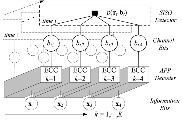
Figure 1: Graphical model of a coded multiuser channel. Note the time dependency among bits of the same user (code constraint), and the user dependency among bits at the same time (channel constraint).

From Fig. 1, it is seen that the nodes representing the channel bits $\{b_{t,k}\}_{k=1}^{K}$ are the relay nodes that separate the graph into two halves, where on one side the decoder runs belief propagation to perform per-user APP decoding and on the other side the multiuser detector performs variational inference. The process by which the APP decoder retrieves prior information and generates extrinsic information is standard (see [9]) and will be skipped. We will therefore only discuss message passing between the detector and decoder.

3.1 Obtaining Extrinsic Information: Sequential Schedule

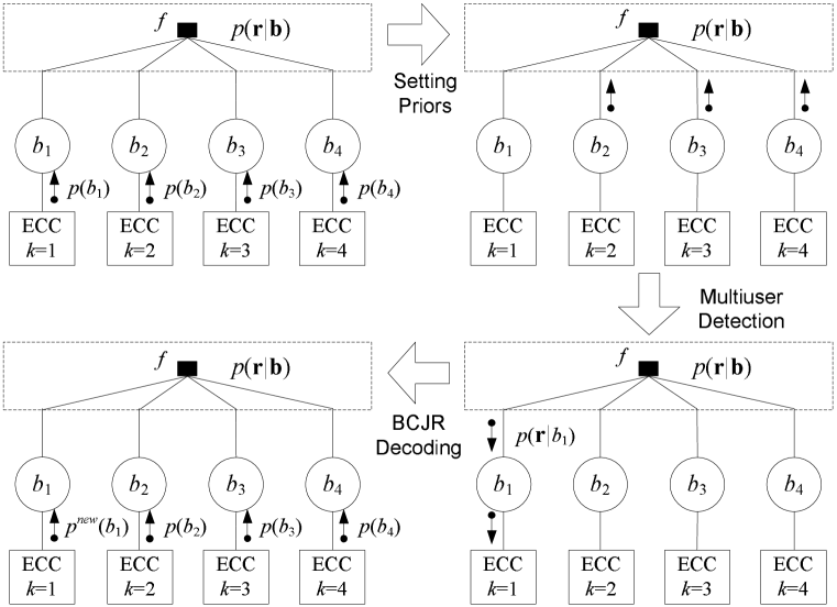
Figure 2: An instance of sequential message-passing in the graphical model: the multiuser detector receives prior distributions of $b_{2}$, $b_{3}$ and $b_{4}$ to generate the extrinsic information for $b_{1}$. This process is repeated for $b_{2}$, $b_{3}$ and $b_{4}$ to complete one message-passing iteration.

When a SISO detector is viewed as an approximate sum-product algorithm [12], the EXT may be obtained in a way analogous to the message-passing rule in graphs. Fig. 2 provides an example that demonstrates that the EXT for $b_{1}$ may be generated using the priors of $b_{2}$, $b_{3}$ and $b_{4}$, but not the prior of $b_{1}$. In its exact form the message (EXT) from node $f$ to node $b_{1}$ is

$$\mathcal{M}_{f\rightarrow b_{1}}=\sum_{b_{2},b_{3},b_{4}}p(\mathbf{r}|\mathbf{b})p(b_{2})p(b_{3})p(b_{4})=p(\mathbf{r}|b_{1}).$$ (6)

In sequential scheduling, $\mathcal{M}_{f\rightarrow b_{1}}$ will be passed into the APP decoder for user 1, which will generate a new prior for $b_{1}$ that will be used for EXT generation for $b_{2}$, and so on. So error control decoding is performed one user at a time, and not in parallel.

In an approximate evaluation of EXT for $b_{k}$ that follows the same vein, one would ignore the prior of $b_{k}$ even if it is available from a previous iteration, and use a simple multi-user detector such as linear MMSE to generate an estimated $p(\mathbf{r}|b_{k})$ using only $\{p(b_{l})\}_{l\neq k}$. Thus in the sequential schedule,

• the EXT for each bit is obtained using different inputs (prior distributions), necessitating a substantially different EXT generator (multiuser detector) for each bit; and

• the prior knowledge of $b_{k}$ is ignored before detection in generating the EXT for $b_{k}$.

The sequential schedule to obtain extrinsic information is intuitive, since it resembles the message-passing protocol defined in the sum-product algorithm [20, ch. 4]. But it is also very restrictive, in that users have to be detected in series, introducing latency in the detection process. Furthermore, since a different joint detector must be devised for each user, the overall complexity in general increases linearly with $K$ if no simplification measures are taken.

3.2 Obtaining Extrinsic Information: Flooding Schedule

Figure 3: An instance of flooding message-passing in the graphical model: the multiuser detector receives prior distributions of $b_{1},\cdots,b_{4}$ to generate the extrinsic information for $b_{1},\cdots,b_{4}$. This completes one message-passing iteration.

In the flooding schedule, illustrated in Fig. 3, EXT’s for all bits are generated in parallel. The message from node $f$ to $b_{k}$ will be

$$\mathcal{M}_{f\rightarrow b_{k}}=\sum_{\{b_{l}\}_{l\neq k}}p(\mathbf{r}|\mathbf{b})\prod_{l=1,l\neq k}^{K}p(b_{l})\propto\frac{p(b_{k}|\mathbf{r})}{p(b_{k})}.$$ (7)

Note that, unlike in sequential scheduling, all EXT’s use the same priors. For instance, $\mathcal{M}_{f\rightarrow b_{2}}$ and $\mathcal{M}_{f\rightarrow b_{4}}$ both use $p(b_{3})$ whereas in the sequential schedule, $\mathcal{M}_{f\rightarrow b_{4}}$ would use $p^{new}(b_{3})$ from the most recent round of APP decoding.

As well, we can write the EXT of $b_{k}$ as

$$\mathcal{M}_{f\rightarrow b_{k}}=\frac{1}{p(b_{k})}\sum_{\{b_{l}\}_{l\neq k}}p(\mathbf{r}|\mathbf{b})\prod_{l=1}^{K}p(b_{l})$$ (8)

and hence view the flooding schedule as making use of all prior probabilities from the same iteration. This reasoning, together with (7), leads to the following sub-optimal approximation:

• Use all prior probabilities from the same iteration to generate an approximate $p(b_{k}|\mathbf{r})$, say $Q(b_{k})$;

• Form the EXT for $b_{k}$ by dividing $Q(b_{k})$ by $p(b_{k})$;

• Send all EXT’s to the $K$ APP decoders in parallel.

The advantage of the flooding schedule is two fold: 1) By passing messages to the detector in one shot, the latency is low; 2) By generating the extrinsic information in one shot, the complexity of the detector is reduced.

Through implementing the flooding schedule, our MUD design challenge is shifted from approximating $p(\mathbf{r}|b_{k})$ to approximating $p(b_{k}|\mathbf{r})$. And the variational inference viewpoint of MUD allows us to easily do so.

3.3 Obtaining Extrinsic Information: Hybrid Schedule

A hybrid schedule can be defined in which the EXT for $b_{k}$ is computed without using $p(b_{k})$ like in the sequential schedule, and all EXT’s are computed in parallel like in the flooding schedule. This approach removes the latency issue in sequential scheduling, and has been used in the literature without justification.

If exact inference is used to compute $p(\mathbf{r}|b_{k})$ in the hybrid schedule, and $p(b_{k}|\mathbf{r})$ in the flooding schedule, the two implementations are identical, since the messages coming out of the MUD section are the same – $\{p(\mathbf{r}|b_{k})\}_{k=1}^{K}$. However, in practical detector design, $p(\mathbf{r}|b_{k})$ or $p(b_{k}|\mathbf{r})$ must be approximated. As to be demonstrated in Section 4.4, $p(b_{k}|\mathbf{r})$ may be approximated as $Q(b_{k})$ given prior distributions $\{p(b_{l})\}_{l=1}^{K}$, while $p(\mathbf{r}|b_{k})$ may be approximated as $Q(b_{k})$ given $\{p(b_{l})\}_{l\neq k}$ and non-informative $p(b_{k})$. With these approximations, the hybrid and flooding scheduling schemes differ, as the former becomes the Wang-Poor turbo detector [3] and the latter turns into a brand-new design.

4 Multiuser Detection via Variational Inference

In [14], Guo and Verdú treat the linear multiuser detectors as posterior mean estimators (PME) with appropriately postulated distributions $p(\mathbf{b})$ and $p(\mathbf{r}|\mathbf{b})$. For example, if a Gaussian prior is assumed, i.e., $p(\mathbf{b})=\mathcal{N}(\mathbf{0},\mathbf{I})$, and the channel is modelled as $p(\mathbf{r}|\mathbf{b})=\mathcal{N}(\mathbf{S}\mathbf{A}\mathbf{b},\alpha^{2}\mathbf{I})$, the posterior (or conditional) mean estimator, i.e., $\mathop{\sf E}\left[\mathbf{b}|\mathbf{r}\right]$, is a generalized linear detector given by

$$\hat{\mathbf{b}}=\left(\mathbf{A}^{T}\mathbf{S}^{T}\mathbf{S}\mathbf{A}+\alpha^{2}\mathbf{I}\right)^{-1}\mathbf{A}^{T}\mathbf{S}^{T}\mathbf{r}.$$ (9)

By choosing different values for $\alpha$, we arrive at different linear detectors. If $\alpha^{2}=\sigma^{2}$, we get the MMSE detector. If $\alpha\rightarrow 0$, we approach the decorrelating detector. And if $\alpha\rightarrow\infty$, the matched filter output is attained.

However, [14] has not considered another important class of detectors, namely the nonlinear detectors. In this work, we wish to extend the coverage of the posterior mean estimator to nonlinear detectors by introducing an additional degree of freedom in approximating the posterior distribution. More specifically, we will not limit ourselves to applying Bayes rule to calculate the posterior, but instead use the more general and flexible variational inference technique.

4.1 Variational Inference and Variational Free Energy Minimization

We shall explain the variational inference method specifically in terms of its application to multiuser detection, while a more general and in-depth treatment, as well as its alternative interpretations and connection to statistical physics, can be found in [21], [22], and [10].

As stated earlier, the general task of the SISO multiuser detector is to perform inference on $\mathbf{b}$ given the observation $\mathbf{r}$, $\mathbf{y}$ or $\bar{\mathbf{y}}$ (we will simply use $\mathbf{r}$ for now, as it is understood that they are equivalent). Suppose our objective is the jointly optimal detector, then the distribution of interest is $p(\mathbf{b}|\mathbf{r})$. Very often, however, the direct evaluation of $p(\mathbf{b}|\mathbf{r})$ is computationally intractable when Bayes rule is applied directly, in particular, when $p(\mathbf{b})$ is a discrete distribution. In such a case, the variational inference technique assumes a tractable approximation to $p(\mathbf{b}|\mathbf{r})$, written as $Q(\mathbf{b})$, where the constant $\mathbf{r}$ is omitted for convenience.

A good approximation $Q(\mathbf{b})$ needs to resemble $p(\mathbf{b}|\mathbf{r})$ as closely as possible, and the Kullback-Leibler divergence (or relative entropy) $\mathbb{D}\left[Q(\mathbf{b})\|p(\mathbf{b}|\mathbf{r})\right]$ offers an excellent measure of similarity. But since the distribution $p(\mathbf{b}|\mathbf{r})$ is difficult to attain as we have assumed, an equivalent alternative, $p(\mathbf{b},\mathbf{r})=p(\mathbf{r}|\mathbf{b})p(\mathbf{b})$, is used, and $p(\mathbf{b},\mathbf{r})$ is called the complete likelihood function. The variational free energy is thus defined as:

$$\mathcal{F}(\lambda)=\int_{\mathbf{b}}Q(\mathbf{b};\lambda)\log\frac{Q(\mathbf{b};\lambda)}{p(\mathbf{b},\mathbf{r})}d\mathbf{b},$$ (10)

which equals $D\left[Q(\mathbf{b})\|p(\mathbf{b}|\mathbf{r})\right]$ up to an additive constant. In (10), $Q(\mathbf{b})$ is written as $Q(\mathbf{b};\lambda)$ to denote the dependence of $Q(\mathbf{b})$ on $\lambda$ explicitly, where $\lambda$ contains a set of parameters that specify $Q(\mathbf{b})$. In the rest of the paper, we will however drop the dependence of the $Q$ function on $\lambda$ in accordance with the usual convention for writing probability distributions.

If no constraints are placed on $Q(\mathbf{b})$, by minimizing $\mathcal{F}(\lambda)$, we reach $Q(\mathbf{b})=p(\mathbf{b}|\mathbf{r})$ and nothing is gained. But if we parameterize $Q(\mathbf{b})$ by assuming that it comes from a restricted family of distributions (for example, a Gaussian), we may very easily find a closed-form expression for $\mathcal{F}(\lambda)$, which leads to a good approximation of $p(\mathbf{b}|\mathbf{r})$ via the minimization of variational free energy. This method of performing approximate inference is called variational inference.

One important technique often used in variational inference is the assumption that $Q(\mathbf{b})$ is factorizable as $\prod_{k=1}^{K}Q_{k}(b_{k})$ (we shall omit the subscripts in $Q_{k}$ from here on), and find distributions $\{Q(b_{k})\}_{k=1}^{K}$ that minimize the free energy. This factorization of a distribution and the independence assumption associated with it is referred to as the mean-field approximation in statistical physics. A demonstration of its application will be presented in detail in Section 4.5.

The following is an outline of the general procedure for deriving multiuser detectors through VFEM:

1. Postulation: Assume postulated distributions for $p(\mathbf{b})$, $p(\mathbf{r}|\mathbf{b})$ and $Q(\mathbf{b})$;

2. Evaluation: Derive closed-form expression for $\mathcal{F}(\lambda)$;

3. Optimization: Minimize $\mathcal{F}(\lambda)$ (exactly or iteratively) over $\lambda$.

Note that we have now transformed the general MUD problem into a well-defined optimization problem, with a unique objective function, called variational free energy. This procedure bears close resemblance to the routine of deriving thermodynamic state equations in statistical physics [23], which is not surprising, considering the fact that variational inference is indeed rooted in statistical physics.

4.2 VFEM Interpretation of Linear Multiuser Detectors

We shall begin by deriving linear multiuser detectors from variational free energy minimization, and thus show that simply adjusting the postulated distributions $p(\mathbf{b})$, $p(\mathbf{r}|\mathbf{b})$ and $Q(\mathbf{b})$ leads to the well-known decorrelating and MMSE detectors. Although the exercises presented here are somewhat trivial, since uncoded linear MUD is the simplest instance of MUD, they lay the foundation for more sophisticated variations in later sections.

Proposition 1

Decorrelating Detectors may be derived through the VFEM routine by assuming the following distributions:

$$\left\{\begin{array}[]{rcl}p(\mathbf{b})&=&Constant\\ p(\mathbf{r}|\mathbf{b})&=&\mathcal{N}(\mathbf{S}\mathbf{A}\mathbf{b},\sigma^{2}\mathbf{I})\\ Q(\mathbf{b})&=&\mathcal{N}(\boldsymbol{\mu},\mathbf{\Sigma}).\end{array}\right.$$ (11)

Proof: Evaluating $\mathcal{F}(\lambda)$ as in (10), we have a function of $\boldsymbol{\mu}$ and $\mathbf{\Sigma}$:

$$\mathcal{F}(\boldsymbol{\mu},\mathbf{\Sigma})=-\frac{1}{2}\log|\mathbf{\Sigma}|+\frac{1}{2\sigma^{2}}\left\{\boldsymbol{\mu}^{T}\mathbf{A}^{T}\mathbf{S}^{T}\mathbf{S}\mathbf{A}\boldsymbol{\mu}+\mathop{\sf tr}[(\mathbf{A}^{T}\mathbf{S}^{T}\mathbf{S}\mathbf{A})\mathbf{\Sigma}]-2\mathbf{r}^{T}\mathbf{S}\mathbf{A}\boldsymbol{\mu}\right\}$$ (12)

The final estimate of $Q(\mathbf{b})$ is given by the minimizers $\hat{\boldsymbol{\mu}}$ and $\hat{\mathbf{\Sigma}}$ of $\mathcal{F}(\boldsymbol{\mu},\mathbf{\Sigma})$. Calculating $\partial\mathcal{F}(\boldsymbol{\mu})/\partial\boldsymbol{\mu}$ and $\partial\mathcal{F}(\mathbf{\Sigma})/\partial\mathbf{\Sigma}^{-1}$ and equating to zero, we have

$$\begin{array}[]{rcl}\hat{\boldsymbol{\mu}}&=&(\mathbf{A}^{T}\mathbf{S}^{T}\mathbf{S}\mathbf{A})^{-1}\mathbf{A}^{T}\mathbf{S}^{T}\mathbf{r}\\ \hat{\mathbf{\Sigma}}&=&\sigma^{2}(\mathbf{A}^{T}\mathbf{S}^{T}\mathbf{S}\mathbf{A})^{-1}.\end{array}$$ (13)

If hard decisions are desired, $\hat{\boldsymbol{\mu}}$ can be used as the detector output, since it maximizes $Q(\mathbf{b})$, which is Gaussian. It is easy to recognize that $\hat{\boldsymbol{\mu}}$ is identical to the decorrelating detector output.   

Note that given the postulated priors in (11), the exact posterior $p(\mathbf{b}|\mathbf{r})$ is tractable and is in fact Gaussian. Therefore, the solved $Q$ function, $\mathcal{N}(\hat{\boldsymbol{\mu}},\hat{\mathbf{\Sigma}})$, is the exact posterior distribution which could also have been found by applying Bayes rule directly.

The decorrelating detector uses non-informative priors for the data bits transmitted, by setting $p(\mathbf{b})$ to a constant. But in practice, side information is available. For instance, $\{b_{k}\}_{k=1}^{K}$ can be safely assumed to be i.i.d. and zero mean. For BPSK signaling, in particular, we also known that $\textsf{E}(b_{k}^{2})=1$. We will subsequently show that the Gaussian approximation about $p(\mathbf{b})$, utilizing the first and second order statistics of $\mathbf{b}$, gives rise to the familiar MMSE detector.

Proposition 2

MMSE Multiuser Detectors may be derived through the VFEM routine by assuming the following distributions:

$$\left\{\begin{array}[]{rcl}p(\mathbf{b})&=&\mathcal{N}(\mathbf{0},\mathbf{I})\\ p(\mathbf{r}|\mathbf{b})&=&\mathcal{N}(\mathbf{S}\mathbf{A}\mathbf{b},\sigma^{2}\mathbf{I})\\ Q(\mathbf{b})&=&\mathcal{N}(\boldsymbol{\mu},\mathbf{\Sigma}).\end{array}\right.$$ (14)

Proof: Evaluating $\mathcal{F}(\lambda)$ yields a function of $\boldsymbol{\mu}$ and $\mathbf{\Sigma}$:

$$\mathcal{F}(\boldsymbol{\mu},\mathbf{\Sigma})=-\frac{1}{2}\log|\mathbf{\Sigma}|+\frac{1}{2\sigma^{2}}\left\{\boldsymbol{\mu}^{T}(\mathbf{A}^{T}\mathbf{S}^{T}\mathbf{S}\mathbf{A}+\sigma^{2}\mathbf{I})\boldsymbol{\mu}+\mathop{\sf tr}[(\mathbf{A}^{T}\mathbf{S}^{T}\mathbf{S}\mathbf{A}+\sigma^{2}\mathbf{I})\mathbf{\Sigma}]-2\mathbf{r}^{T}\mathbf{S}\mathbf{A}\boldsymbol{\mu}\right\}$$ (15)

Solving $\partial\mathcal{F}(\boldsymbol{\mu})/\partial\boldsymbol{\mu}=\mathbf{0}$ and $\partial\mathcal{F}(\mathbf{\Sigma})/\partial\mathbf{\Sigma}^{-1}=\mathbf{0}$ leads to the following solution:

$$\begin{array}[]{rcl}\hat{\boldsymbol{\mu}}&=&(\mathbf{A}^{T}\mathbf{S}^{T}\mathbf{S}\mathbf{A}+\sigma^{2}\mathbf{I})^{-1}\mathbf{A}^{T}\mathbf{S}^{T}\mathbf{r}\\ \hat{\mathbf{\Sigma}}&=&\sigma^{2}(\mathbf{A}^{T}\mathbf{S}^{T}\mathbf{S}\mathbf{A}+\sigma^{2}\mathbf{I})^{-1}.\end{array}$$ (16)

Apparently, $\hat{\boldsymbol{\mu}}$ in (16) can be identified as the MMSE detector output.   

Note that the variational inference interpretation of decorrelating and MMSE detectors also produces a covariance matrix $\mathbf{\Sigma}$ of the $Q$ function, which is not available through conventional signal processing techniques. $\mathbf{\Sigma}$ indicates the reliability of the detector output, something the hard-decision detector is unable to make use of. But it will prove valuable in SISO detectors, as demonstrated in Sections 4.4 and 4.5.

4.3 VFEM Interpretation of Interference Cancellation Detectors

Iterative multiuser detectors, and especially their convergence behavior, have been actively researched in the past. In [24], linear SIC and PIC are categorized as the Gauss-Seidel and Jacobi iterations for solving linear equations. SIC is also analyzed in greater depth in [25] and [26]. The study is later extended to clipped SIC in [27] through the investigation of the variational inequality (VI) problem. Here we offer an alternative view of SIC as the coordinate descent algorithm applied to the minimization of $\mathcal{F}(\boldsymbol{\mu},\mathbf{\Sigma})$.

Proposition 3

Linear/Clipped SIC Detectors may be derived from assuming the same distributions as in (11) or (14), except by minimizing $\mathcal{F}(\boldsymbol{\mu},\mathbf{\Sigma})$ using the coordinate descent algorithm. That is, in the $i$-th iteration, for $k=1$ to $K$,

$$\begin{array}[]{cl}\min_{\mu_{k}}&\mathcal{F}(\mu_{1}^{(i)},\cdots,\mu_{k-1}^{(i)},\mu_{k},\mu_{k+1}^{(i-1)},\cdots,\mu_{K}^{(i-1)},\mathbf{\Sigma})\\ $s.t.$&\mu_{min}\leq\mu_{k}\leq\mu_{max}.\end{array}$$ (17)

The algorithm describes a linear SIC if $\mu_{min}=-\infty$ and $\mu_{max}=\infty$, and a clipped SIC otherwise.

Proof: Setting $\partial\mathcal{F}(\boldsymbol{\mu},\mathbf{\Sigma})/\partial\mu_{k}=0$ based on (15) yields

$$A_{k}\mathbf{s}_{k}^{T}\mathbf{S}\mathbf{A}\boldsymbol{\mu}-A_{k}\mathbf{s}_{k}^{T}\mathbf{r}+\sigma^{2}\mu_{k}=0.$$ (18)

Rearranging the terms and defining $\boldsymbol{\mu}_{\setminus k}=[\mu_{1},\cdots,\mu_{k-1},0,\mu_{k+1},\cdots,\mu_{K}]^{T}$, the optimal $\mu_{k}$ is then expressed in the familiar linear interference cancellation form if $\mu_{k}$ is unbounded (i.e., $\mu_{min}=-\infty$ and $\mu_{max}=\infty$):

$$\hat{\mu}_{k}=\frac{1}{A_{k}^{2}+\sigma^{2}}A_{k}\mathbf{s}_{k}^{T}(\mathbf{r}-\mathbf{S}\mathbf{A}\boldsymbol{\mu}_{\setminus k}).$$ (19)

Since updating $\mu_{k}$ ($k=1,\cdots,K$) consecutively subject to $\partial\mathcal{F}(\boldsymbol{\mu},\mathbf{\Sigma})/\partial\mu_{k}=0$ is the coordinate descent algorithm for minimizing $\mathcal{F}(\boldsymbol{\mu},\mathbf{\Sigma})$, then (19) corresponds to the coordinate descent implementation of the MMSE detector. On the other hand, setting $\partial\mathcal{F}(\boldsymbol{\mu},\mathbf{\Sigma})/\partial\mu_{k}=0$ based on (12) leads to the the coordinate descent implementation of the decorrelating detector:

$$\hat{\mu}_{k}=\frac{1}{A_{k}}\mathbf{s}_{k}^{T}(\mathbf{r}-\mathbf{S}\mathbf{A}\boldsymbol{\mu}_{\setminus k}),$$ (20)

which is the standard-form SIC detector seen in the literature. If $\mu_{min}$ and $\mu_{max}$ are finite, we need to solve (18) subject to $\mu_{min}\leq\mu_{k}\leq\mu_{max}$, which corresponds to clipped SIC.   

To verify that (19) and (20) do converge to MMSE or decorrelator solutions, and to gain further insights into the convergence behavior when the optimization constraints are active (clipped SIC), we invoke the following theorem [28]:

Theorem 1 (Luo and Tseng, 1992)

Consider an optimization problem:

$$\begin{array}[]{ll}min\ f(\mathbf{x})=g(\mathbf{E}\mathbf{x})+\mathbf{c}^{T}\mathbf{x},&s.t.\ \mathbf{x}\in\mathcal{X},\end{array}$$ (21)

where $\mathcal{X}$ is a box (possibly unbounded) in $\mathbb{R}^{n}$, $f$ is a proper closed convex function in $\mathbb{R}^{n}$, $g$ is a proper closed convex function in $\mathbb{R}^{m}$, $\mathbf{E}$ is an $m\times n$ matrix having no zero column, and $\mathbf{c}\in\mathbb{R}^{n}$. Also assume

1. The set of optimal solutions for (21), denoted by $\mathcal{X}^{*}$ is nonempty;

2. The domain of $g$ is open and $g$ is strictly convex twice continuously differentiable on the domain;

3. $\nabla^{2}g(\mathbf{E}\mathbf{x}^{*})$ is positive definite for all $\mathbf{x}^{*}\in\mathcal{X}^{*}$.

Then if $\{\mathbf{x}^{r}\}$ is a sequence of iterates generated by coordinate descent method according to the Almost Cyclic Rule or Gauss-Southwell Rule, $\{\mathbf{x}^{r}\}$ converges at least linearly to an element of $\mathcal{X}^{*}$.

Since the objective function of optimization, $\mathcal{F}(\boldsymbol{\mu},\mathbf{\Sigma})$, satisfies all conditions in the theorem when the spreading codes are linearly independent, it is clear that this theorem applies to the general linear/clipped SIC setting. Also due to the objective function being quadratic and the constraints being linear, there is a unique optimal solution in $\mathcal{X}^{*}$. We may thus conclude the following:

Corollary 1

Linear/Clipped SIC are guaranteed to converge to the unique minimum free energy defined by $\mathcal{F}(\boldsymbol{\mu},\mathbf{\Sigma})$ and the constraint ($\mu_{min}\leq\mu_{k}\leq\mu_{max}$), and the rate of convergence is at least linear.

This result is proven for the first time to our knowledge. Additionally, we may relax the conventional cyclic order of iteration for SIC and assert that as long as the coordinates are iterated upon according to either the Almost Cyclic Rule or Gauss-Southwell Rule, at least linear convergence rate is guaranteed. These relaxed iteration rules are discussed in [28].

In the sequel, we will investigate a few SISO multiuser detectors within the variational inference framework. Unlike the uncoded detectors studied previously, we will now make use of the soft output provided by $Q(\mathbf{b})$ to facilitate iterative multiuser joint decoding. We will demonstrate that a unique SISO detector is determined by choosing 1) the postulated distributions (like (11) and (14), but with biased priors), and 2) the message-passing schedule for joint decoding.

4.4 VFEM Interpretation of Gaussian SISO Multiuser Detector

Definition 1

A Gaussian SISO Multiuser Detector is a multiuser detector that obtains soft estimates $Q(\mathbf{b})$ through the VFEM routine, subject to the following postulated distributions: $$\left\{\begin{array}[]{rcl}p(\mathbf{b})&=&\mathcal{N}(\tilde{\mathbf{b}},\mathbf{W})\\ p(\mathbf{r}|\mathbf{b})&=&\mathcal{N}(\mathbf{S}\mathbf{A}\mathbf{b},\sigma^{2}\mathbf{I})\\ Q(\mathbf{b})&=&\mathcal{N}(\boldsymbol{\mu},\mathbf{\Sigma}),\end{array}\right.$$ (22) where $\tilde{\mathbf{b}}=[\tilde{b}_{1},\cdots,\tilde{b}_{K}]^{T}$ are the soft bit estimates from the APP decoder, and $\mathbf{W}=\mathop{\sf diag}([1-\tilde{b}_{1}^{2},\cdots,1-\tilde{b}_{K}^{2}]^{T})$.

We name this detector Gaussian SISO MUD because, like the uncoded linear detectors in Section 4.2, Gaussian densities are assumed for the prior and posterior distributions of $\mathbf{b}$. But unlike the linear detectors, this detector is capable of accepting informative priors, as well as generating soft posterior bit probability.

4.4.1 The Existing Form of Gaussian SISO MUD

A ground-breaking turbo detection scheme was proposed by Wang and Poor [3], spurring a tremendous amount of interest in turbo MUD and turbo equalization in the years that followed. It involves a two stage process: First, the soft bit estimate from the APP decoder is remodulated and subtracted from the matched filter output:

$$\mathbf{y}_{k}\triangleq\mathbf{y}-\mathbf{R}\mathbf{A}\tilde{\mathbf{b}}_{k},$$ (23)

In (23), $\tilde{\mathbf{b}}_{k}=[\tilde{b}_{1},\cdots,\tilde{b}_{k-1},0,\tilde{b}_{k+1},\cdots,\tilde{b}_{K}]^{T}$, which is equal to the soft bit estimates coming from the APP decoder, $\tilde{\mathbf{b}}$, except for the $k$-th element being $0$.

Second, a linear MMSE filter is used to further suppress the residual interference. It can be shown that the filter output is

$$z_{k}=A_{k}\mathbf{e}_{k}^{T}\overbrace{\left[\mathbf{A}^{T}\mathbf{W}_{k}\mathbf{A}+\sigma^{2}\mathbf{R}^{-1}\right]^{-1}}^{\mbox{MMSE with residual MAI}}\overbrace{\left[\mathbf{R}^{-1}\mathbf{y}-\mathbf{A}\tilde{\mathbf{b}}_{k}\right]}^{\mbox{Soft IC}},$$ (24)

where $\mathbf{e}_{k}$ denotes a $K$-vector of all zeros, except for the $k$-th element being $1$, and $\mathbf{W}_{k}=\mathop{\sf diag}([1-\tilde{b}_{1}^{2},\cdots,1-\tilde{b}_{k-1}^{2},1,1-\tilde{b}_{k+1}^{2},\cdots,1-\tilde{b}_{K}^{2}]^{T})$.

In order to convert the MMSE filter output $z_{k}$ into a soft estimate in the discrete domain, a Gaussian equivalent channel assumption is made about $z_{k}$, i.e.,

$$z_{k}=\alpha_{k}b_{k}+\eta_{k},$$ (25)

where $\alpha_{k}$ is a constant and $p(\eta_{k})=\mathcal{N}(0,\nu_{k}^{2})$. In other words, $p(z_{k}|b_{k})=\mathcal{N}(\alpha_{k}b_{k},\nu_{k}^{2})$. Since $\alpha_{k}$ and $\nu_{k}^{2}$ can be found to be, respectively,

$$\begin{array}[]{rcl}\alpha_{k}&=&A_{k}^{2}\left[(\mathbf{A}^{T}\mathbf{W}_{k}\mathbf{A}+\sigma^{2}\mathbf{R}^{-1})^{-1}\right]_{k,k}\\ \nu_{k}^{2}&=&z_{k}-z_{k}^{2},\end{array}$$ (26)

the output EXT can be written as

$$\mbox{LLR}_{mud}(b_{k})=\log\frac{p(\mathbf{r}|b_{k}=1)}{p(\mathbf{r}|b_{k}=-1)}\thickapprox\log\frac{p(z_{k}|b_{k}=1)}{p(z_{k}|b_{k}=-1)}=\frac{2z_{k}}{1-\alpha_{k}}.$$ (27)

In essence, the target distribution $p(\mathbf{r}|b_{k})$ is approximated by $p(z_{k}|b_{k})$ to obtain the EXT. We will now demonstrate that with the VFEM formulation, the two-stage process can be derived from a single optimization procedure, and without the heuristic Gaussian assumption about $z_{k}$.

Proposition 4

The SISO multiuser detection scheme described in [3] is an instance of Gaussian SISO MUD.

Proof: If the extrinsic information is extracted following the sequential schedule in Section 3.1, by ignoring the prior information for $b_{k}$, then (22) may be modified as

$$\left\{\begin{array}[]{rcl}p(\mathbf{b})&=&\mathcal{N}(\tilde{\mathbf{b}}_{k},\mathbf{W}_{k})\\ p(\mathbf{r}|\mathbf{b})&=&\mathcal{N}(\mathbf{S}\mathbf{A}\mathbf{b},\sigma^{2}\mathbf{I})\\ Q(\mathbf{b})&=&\mathcal{N}(\boldsymbol{\mu}_{k},\mathbf{\Sigma}_{k}),\end{array}\right.$$ (28)

where $\tilde{\mathbf{b}}_{k}=[\tilde{b}_{1},\cdots,\tilde{b}_{k-1},0,\tilde{b}_{k+1},\cdots,\tilde{b}_{K}]^{T}$ and $\mathbf{W}_{k}=\mathop{\sf diag}([1-\tilde{b}_{1}^{2},\cdots,1-\tilde{b}_{k-1}^{2},1,1-\tilde{b}_{k+1}^{2},\cdots,1-\tilde{b}_{K}^{2}]^{T})$. From (28), it can be shown that

$$\begin{array}[]{rcl}\mathcal{F}_{gauss}(\boldsymbol{\mu}_{k},\mathbf{\Sigma}_{k})&=&\frac{1}{2\sigma^{2}}[\boldsymbol{\mu}_{k}^{T}(\mathbf{A}^{T}\mathbf{S}^{T}\mathbf{S}\mathbf{A}+\sigma^{2}\mathbf{W}_{k}^{-1})\boldsymbol{\mu}_{k}-2(\mathbf{r}^{T}\mathbf{S}\mathbf{A}+\sigma^{2}\tilde{\mathbf{b}}_{k}^{T}\mathbf{W}_{k}^{-1})\boldsymbol{\mu}_{k}]\\ &&-\frac{1}{2}\log|\mathbf{\Sigma}_{k}|+\frac{1}{2}\mathop{\sf tr}(\mathbf{W}_{k}^{-1}\mathbf{\Sigma}_{k})+\frac{1}{2\sigma^{2}}\mathop{\sf tr}(\mathbf{A}^{T}\mathbf{S}^{T}\mathbf{S}\mathbf{A}\mathbf{\Sigma}_{k}).\end{array}$$ (29)

Let $\mu_{k}^{\prime}$ denote the $k$-th element of $\boldsymbol{\mu}_{k}$. Solving $\partial\mathcal{F}_{gauss}(\boldsymbol{\mu}_{k},\mathbf{\Sigma}_{k})/\partial\mu_{k}^{\prime}=0$ yields

$$\mu_{k}^{\prime}=\mathbf{e}_{k}^{T}(\mathbf{A}^{T}\mathbf{S}^{T}\mathbf{S}\mathbf{A}+\sigma^{2}\mathbf{W}_{k}^{-1})^{-1}\mathbf{A}^{T}\mathbf{S}^{T}(\mathbf{r}-\mathbf{S}\mathbf{A}\tilde{\mathbf{b}}_{k}),$$ (30)

which is identical to $z_{k}$ in (24).

One piece of information that the MMSE-based detector in [3] does not have is the covariance matrix of the posterior distribution, $\mathbf{\Sigma}_{k}$, which can be shown to be

$$\mathbf{\Sigma}_{k}=\left(\frac{1}{\sigma^{2}}\mathbf{A}^{T}\mathbf{S}^{T}\mathbf{S}\mathbf{A}+\mathbf{W}_{k}^{-1}\right)^{-1}.$$ (31)

In other words, the marginal posterior distribution of $b_{k}$ is $Q(b_{k})=\mathcal{N}(\mu_{k}^{\prime},[\mathbf{\Sigma}_{k}]_{k,k})$. Since the prior distribution of $b_{k}$ is ignored during the detection operation, $Q(b_{k})$ obtained as such is in fact proportional to $p(\mathbf{r}|b_{k})$. Therefore,

$$\mbox{LLR}_{mud}(b_{k})=\log\frac{p(\mathbf{r}|b_{k}=1)}{p(\mathbf{r}|b_{k}=-1)}\thickapprox\log\frac{Q(b_{k}=1)}{Q(b_{k}=-1)}=\frac{2\mu_{k}^{\prime}}{[\mathbf{\Sigma}_{k}]_{k,k}}.$$ (32)

Applying the matrix inversion lemma on $\mathbf{\Sigma}_{k}$ in (31), we have

$$\mathbf{\Sigma}_{k}=\mathbf{W}_{k}-\mathbf{W}_{k}\mathbf{A}(\mathbf{A}\mathbf{W}_{k}\mathbf{A}+\sigma^{2}\mathbf{R}^{-1})^{-1}\mathbf{A}\mathbf{W}_{k}.$$ (33)

Since $[\mathbf{W}_{k}]_{k,k}=1$, $[\mathbf{\Sigma}_{k}]_{k,k}=1-A_{k}^{2}[(\mathbf{A}\mathbf{W}_{k}\mathbf{A}+\sigma^{2}\mathbf{R}^{-1})^{-1}]_{k,k}=1-\alpha_{k}$, where $\alpha_{k}$ is as defined in (26). Therefore,

$$\mbox{LLR}_{mud}(b_{k})=\frac{2\mu_{k}^{\prime}}{[\mathbf{\Sigma}_{k}]_{k,k}}=\frac{2z_{k}}{1-\alpha_{k}}.$$ (34)

We have thus re-derived the Wang-Poor scheme via a radically different approach. It is remarkable how the variational inference viewpoint leads to exactly the same outcome as [3], while the conditional Gaussian assumption made about the MMSE filter output is no longer necessary.   

After taking APP decoding into account, the Wang-Poor turbo MUD algorithm as a whole can be seen as hybrid-Gaussian-SISO MUD. In the next section, we will systematically investigate all three possible scheduling schemes applied to Gaussian SISO MUD.

4.4.2 The Standard Forms of Gaussian SISO MUD

Table 1: Three scheduling schemes of turbo MUD employing Gaussian SISO MUD.

Sequential-Gaussian-SISO
Initialization: $\tilde{\mathbf{b}}=\mathbf{0}$
FOR $j=1:J$ (Outer Iteration)
	FOR $k=1:K$
		$\tilde{\mathbf{b}}_{k}$	=	$[\tilde{b}_{1},\cdots,\tilde{b}_{k-1},0,\tilde{b}_{k+1},\cdots,\tilde{b}_{K}]^{T}$
		$\mathbf{W}_{k}$	=	$\mathop{\sf diag}([1-\tilde{b}_{1}^{2},\cdots,1-\tilde{b}_{k-1}^{2},1,1-\tilde{b}_{k+1}^{2},\cdots,1-\tilde{b}_{K}^{2}]^{T})$
		$\mu_{k}^{\prime}$	=	$A_{k}\mathbf{e}_{k}^{T}\left[\mathbf{A}^{T}\mathbf{W}_{k}\mathbf{A}+\sigma^{2}\mathbf{R}^{-1}\right]^{-1}\left[\mathbf{R}^{-1}\mathbf{y}-\mathbf{A}\tilde{\mathbf{b}}_{k}\right]$
		$\alpha_{k}$	=	$A_{k}^{2}\left[(\mathbf{A}^{T}\mathbf{W}_{k}\mathbf{A}+\sigma^{2}\mathbf{R}^{-1})^{-1}\right]_{k,k}$
		$\mbox{LLR}_{mud}(b_{k})=\frac{2\mu_{k}^{\prime}}{1-\alpha_{k}}$
		$\mbox{LLR}_{dec}(b_{k})\stackrel{{\scriptstyle\scriptsize\mbox{Decoding}}}{{\Longleftarrow}}\mbox{LLR}_{mud}(b_{k})$
		$\tilde{b}_{k}$	=	$\tanh[\mbox{LLR}_{dec}(b_{k})/2]$
	END
END
Flooding-Gaussian-SISO
Initialization: $\tilde{\mathbf{b}}=\mathbf{0}$
FOR $j=1:J$ (Outer Iteration)
	FOR $k=1:K$
		$\tilde{\mathbf{b}}_{k}$	=	$[\tilde{b}_{1},\cdots,\tilde{b}_{k-1},0,\tilde{b}_{k+1},\cdots,\tilde{b}_{K}]^{T}$
		$\mathbf{W}$	=	$\mathop{\sf diag}([1-\tilde{b}_{1}^{2},\cdots,1-\tilde{b}_{K}^{2}]^{T})$
		$\check{\mu}_{k}$	=	$A_{k}\mathbf{e}_{k}^{T}\left[\mathbf{A}^{T}\mathbf{W}\mathbf{A}+\sigma^{2}\mathbf{R}^{-1}\right]^{-1}\left[\mathbf{R}^{-1}\mathbf{y}-\mathbf{A}\tilde{\mathbf{b}}_{k}\right]$
		$\check{\alpha}_{k}$	=	$(1-\tilde{b}_{k}^{2})A_{k}^{2}\left[(\mathbf{A}^{T}\mathbf{W}\mathbf{A}+\sigma^{2}\mathbf{R}^{-1})^{-1}\right]_{k,k}$
		$\mbox{LLR}_{mud}(b_{k})=\frac{2\check{\mu}_{k}}{1-\check{\alpha}_{k}}$
	END
	FOR $k=1:K$
		$\mbox{LLR}_{dec}(b_{k})\stackrel{{\scriptstyle\scriptsize\mbox{Decoding}}}{{\Longleftarrow}}\mbox{LLR}_{mud}(b_{k})$
		$\tilde{b}_{k}$	=	$\tanh[\mbox{LLR}_{dec}(b_{k})/2]$
	END
END
Hybrid-Gaussian-SISO
Initialization: $\tilde{\mathbf{b}}=\mathbf{0}$
FOR $j=1:J$ (Outer Iteration)
	FOR $k=1:K$
		$\tilde{\mathbf{b}}_{k}$	=	$[\tilde{b}_{1},\cdots,\tilde{b}_{k-1},0,\tilde{b}_{k+1},\cdots,\tilde{b}_{K}]^{T}$
		$\mathbf{W}_{k}$	=	$\mathop{\sf diag}([1-\tilde{b}_{1}^{2},\cdots,1-\tilde{b}_{k-1}^{2},1,1-\tilde{b}_{k+1}^{2},\cdots,1-\tilde{b}_{K}^{2}]^{T})$
		$\mu_{k}^{\prime}$	=	$A_{k}\mathbf{e}_{k}^{T}\left[\mathbf{A}^{T}\mathbf{W}_{k}\mathbf{A}+\sigma^{2}\mathbf{R}^{-1}\right]^{-1}\left[\mathbf{R}^{-1}\mathbf{y}-\mathbf{A}\tilde{\mathbf{b}}_{k}\right]$
		$\alpha_{k}$	=	$A_{k}^{2}\left[(\mathbf{A}^{T}\mathbf{W}_{k}\mathbf{A}+\sigma^{2}\mathbf{R}^{-1})^{-1}\right]_{k,k}$
		$\mbox{LLR}_{mud}(b_{k})=\frac{2\mu_{k}^{\prime}}{1-\alpha_{k}}$
	END
	FOR $k=1:K$
		$\mbox{LLR}_{dec}(b_{k})\stackrel{{\scriptstyle\scriptsize\mbox{Decoding}}}{{\Longleftarrow}}\mbox{LLR}_{mud}(b_{k})$
		$\tilde{b}_{k}$	=	$\tanh[\mbox{LLR}_{dec}(b_{k})/2]$
	END
END

In Table 2, we summarize three different versions of standard Gaussian SISO MUD. In the following, we point out some of the major characteristics associated with each one, and, in particular, introduce the new flooding schedule implementation.

Sequential-Gaussian-SISO: In Section 4.4.1, we presented an elegant variational-inference-based approach to obtain the EXT at the SISO detector output, which coincides with the EXT conventionally calculated through soft interference cancellation and MMSE filtering.

In contrast to [3], however, where the EXT’s are stored until all users are processed and then used for APP decoding in parallel, the sequential schedule requires the EXT, $\mbox{LLR}_{mud}(b_{k})$, be directly passed down to the APP decoder. Then the EXT from the APP decoder, viewed by the detector as the updated prior $\tilde{b}_{k}$, is immediately used for the detection of $b_{k+1}$.

Flooding-Gaussian-SISO: The flooding schedule allows the APP decoding of all users to be done in parallel. In the detection stage, some changes to the derivation presented in Section 4.4.1 are needed, since the prior information of $b_{k}$ should not be ignored as is done in (28). Instead, the postulated distributions in (22) are adopted.

Given (22), the free energy becomes

$$\begin{array}[]{rcl}\mathcal{F}_{gauss}(\boldsymbol{\mu},\mathbf{\Sigma})&=&\frac{1}{2\sigma^{2}}[\boldsymbol{\mu}^{T}(\mathbf{A}^{T}\mathbf{S}^{T}\mathbf{S}\mathbf{A}+\sigma^{2}\mathbf{W}^{-1})\boldsymbol{\mu}-2(\mathbf{r}^{T}\mathbf{S}\mathbf{A}+\sigma^{2}\tilde{\mathbf{b}}^{T}\mathbf{W}^{-1})\boldsymbol{\mu}]\\ &&-\frac{1}{2}\log|\mathbf{\Sigma}|+\frac{1}{2}\mathop{\sf tr}(\mathbf{W}^{-1}\mathbf{\Sigma})+\frac{1}{2\sigma^{2}}\mathop{\sf tr}(\mathbf{A}^{T}\mathbf{S}^{T}\mathbf{S}\mathbf{A}\mathbf{\Sigma}).\end{array}$$ (35)

Solving $\partial\mathcal{F}(\boldsymbol{\mu},\mathbf{\Sigma})/\partial\boldsymbol{\mu}=\mathbf{0}$ and $\partial\mathcal{F}(\boldsymbol{\mu},\mathbf{\Sigma})/\partial\mathbf{\Sigma}^{-1}=\mathbf{0}$ leads to the minimizer of $\mathcal{F}_{gauss}(\boldsymbol{\mu},\mathbf{\Sigma})$ in (29):

$$\begin{array}[]{rcl}\boldsymbol{\mu}&=&\tilde{\mathbf{b}}+(\mathbf{A}^{T}\mathbf{S}^{T}\mathbf{S}\mathbf{A}+\sigma^{2}\mathbf{W}^{-1})^{-1}\mathbf{A}^{T}\mathbf{S}^{T}(\mathbf{r}-\mathbf{S}\mathbf{A}\tilde{\mathbf{b}})\\ \mathbf{\Sigma}&=&(\sigma^{-2}\mathbf{A}^{T}\mathbf{S}^{T}\mathbf{S}\mathbf{A}+\mathbf{W}^{-1})^{-1}.\end{array}$$ (36)

It implies that the approximate posterior distribution, $p(\mathbf{b}|\mathbf{r})\thickapprox Q(\mathbf{b})=\mathcal{N}(\boldsymbol{\mu},\mathbf{\Sigma})$. In other words, the marginal posterior distribution of $b_{k}$ is $p(b_{k}|\mathbf{r})\thickapprox\mathcal{N}(\mu_{k},[\mathbf{\Sigma}]_{k,k})$. Recalling in (22), $p(b_{k})=\mathcal{N}(\tilde{b}_{k},1-\tilde{b}_{k}^{2})$, if we apply the flooding schedule in Section 3.2 to extract the EXT, then

$$p(\mathbf{r}|b_{k})\varpropto\frac{p(b_{k}|\mathbf{r})}{p(b_{k})}\thickapprox\frac{Q(b_{k})}{p(b_{k})}=\mathcal{N}(\mu_{ext},\sigma_{ext}^{2}),$$ (37)

where

$$\begin{array}[]{rcl}\mu_{ext}&=&\sigma_{ext}^{2}\left(\frac{\mu_{k}}{[\mathbf{\Sigma}]_{k,k}}-\frac{\tilde{b}_{k}}{1-\tilde{b}_{k}^{2}}\right)\\ \frac{1}{\sigma_{ext}^{2}}&=&\frac{1}{[\mathbf{\Sigma}]_{k,k}}-\frac{1}{1-\tilde{b}_{k}^{2}}.\end{array}$$ (38)

(38) is true, because if $\mathcal{N}(\mu_{1},\sigma_{1}^{2})\mathcal{N}(\mu_{2},\sigma_{2}^{2})\varpropto\mathcal{N}(\mu_{3},\sigma_{3}^{2})$, then [11]

$$\begin{array}[]{rcl}\frac{\mu_{3}}{\sigma_{3}^{2}}&=&\frac{\mu_{1}}{\sigma_{1}^{2}}+\frac{\mu_{2}}{\sigma_{2}^{2}}\\ \frac{1}{\sigma_{3}^{2}}&=&\frac{1}{\sigma_{1}^{2}}+\frac{1}{\sigma_{2}^{2}}.\end{array}$$ (39)

Finally, sampling $\mathcal{N}(\mu_{ext},\sigma_{ext}^{2})$ at $b_{k}=1$ and $b_{k}=-1$, we obtain

$$\begin{array}[]{rcl}\mbox{LLR}_{mud}(b_{k})&=&\log\frac{p(\mathbf{r}|b_{k}=1)}{p(\mathbf{r}|b_{k}=-1)}\\ &\thickapprox&\frac{2\mu_{ext}}{\sigma_{ext}^{2}}\\ &=&\frac{2\mu_{k}}{[\mathbf{\Sigma}]_{k,k}}-\frac{2\tilde{b}_{k}}{1-\tilde{b}_{k}^{2}}\\ &=&\frac{2\mathbf{e}_{k}^{T}[\tilde{\mathbf{b}}+\mathbf{W}\mathbf{A}(\mathbf{A}\mathbf{W}\mathbf{A}+\sigma^{2}\mathbf{R}^{-1})^{-1}(\mathbf{R}^{-1}\mathbf{y}-\mathbf{A}\tilde{\mathbf{b}})]}{(1-\tilde{b}_{k}^{2})-(1-\tilde{b}_{k}^{2})^{2}A_{k}^{2}\left[(\mathbf{A}\mathbf{W}\mathbf{A}+\sigma^{2}\mathbf{R}^{-1})\right]_{k,k}}-\frac{2\tilde{b}_{k}}{1-\tilde{b}_{k}^{2}}\\ &=&\frac{2\mathbf{e}_{k}^{T}[\mathbf{W}\mathbf{A}(\mathbf{A}\mathbf{W}\mathbf{A}+\sigma^{2}\mathbf{R}^{-1})^{-1}(\mathbf{R}^{-1}\mathbf{y}-\mathbf{A}\tilde{\mathbf{b}}_{k})]-2\tilde{b}_{k}(1-\tilde{b}_{k}^{2})A_{k}^{2}\left[(\mathbf{A}\mathbf{W}\mathbf{A}+\sigma^{2}\mathbf{R}^{-1})\right]_{k,k}}{(1-\tilde{b}_{k}^{2})\left\{1-(1-\tilde{b}_{k}^{2})A_{k}^{2}\left[(\mathbf{A}\mathbf{W}\mathbf{A}+\sigma^{2}\mathbf{R}^{-1})^{-1}\right]_{k,k}\right\}}\\ &=&\frac{2(1-\tilde{b}_{k}^{2})A_{k}\mathbf{e}_{k}^{T}(\mathbf{A}\mathbf{W}\mathbf{A}+\sigma^{2}\mathbf{R}^{-1})^{-1}(\mathbf{R}^{-1}\mathbf{y}-\mathbf{A}\tilde{\mathbf{b}}_{k})}{(1-\tilde{b}_{k}^{2})\left\{1-(1-\tilde{b}_{k}^{2})A_{k}^{2}\left[(\mathbf{A}\mathbf{W}\mathbf{A}+\sigma^{2}\mathbf{R}^{-1})^{-1}\right]_{k,k}\right\}}\\ &=&\frac{2\check{\mu}_{k}}{1-\check{\alpha}_{k}^{2}},\end{array}$$ (40)

where

$$\begin{array}[]{rcl}\check{\mu}_{k}&=&A_{k}\mathbf{e}_{k}^{T}(\mathbf{A}\mathbf{W}\mathbf{A}+\sigma^{2}\mathbf{R}^{-1})^{-1}(\mathbf{R}^{-1}\mathbf{y}-\mathbf{A}\tilde{\mathbf{b}}_{k})\\ \check{\alpha}_{k}&=&(1-\tilde{b}_{k}^{2})A_{k}^{2}\left[(\mathbf{A}\mathbf{W}\mathbf{A}+\sigma^{2}\mathbf{R}^{-1})^{-1}\right]_{k,k}.\end{array}$$ (41)

In (41), $\check{\mu}_{k}$ can also be computed more efficiently as

$$\check{\mu}_{k}=A_{k}\mathbf{e}_{k}^{T}(\mathbf{A}\mathbf{W}\mathbf{A}+\sigma^{2}\mathbf{R}^{-1})^{-1}(\mathbf{R}^{-1}\mathbf{y}-\mathbf{A}\tilde{\mathbf{b}})+\tilde{b}_{k}A_{k}^{2}\left[(\mathbf{A}\mathbf{W}\mathbf{A}+\sigma^{2}\mathbf{R}^{-1})^{-1}\right]_{k,k},$$ (42)

such that common information may be utilized to evaluate $\check{\mu}_{k}$ for all $k$.

Hybrid-Gaussian-SISO: As mentioned earlier, the Wang-Poor turbo MUD scheme is exactly the hybrid-Gaussian-SISO MUD. It differs from the sequential schedule in that the EXT for $b_{k}$ generated by the SISO detector is now stored until the EXT’s of all users $k=1,\cdots,K$ are ready. Then EXT’s are passed down to the APP decoders, for decoding in parallel. Hybrid-Gaussian-SISO MUD brings computational savings compared to the more optimal sequential-Gaussian-SISO MUD, due to both the possibility of parallel decoding, and the ease of evaluating $[\mathbf{A}^{T}\mathbf{W}_{k}\mathbf{A}+\sigma^{2}\mathbf{R}^{-1}]^{-1}$.

So far, based on the Gaussian distributions assumed in the postulation step, we showed that the variational inference algorithm converges to a family of Gaussian SISO detectors, including the well-known Wang-Poor scheme as the special case. But the VFEM framework allows us to generalize even further, since the Gaussian distributions, albeit convenient, are unnatural choices for BPSK symbols. The subsequent section will focus on a different family of detectors induced by a different set of assumptions in the postulation step.

4.5 VFEM Interpretation of Discrete SISO Multiuser Detector

Definition 2

A Discrete SISO Multiuser Detector is a multiuser detector that obtains soft estimates $Q(\mathbf{b})$ through the VFEM routine, subject to the following postulated distributions: $$\left\{\begin{array}[]{rcl}p(\mathbf{b})&=&\prod_{k=1}^{K}\xi_{k}^{\frac{1+b_{k}}{2}}(1-\xi_{k})^{\frac{1-b_{k}}{2}},\ \ b_{k}\in\{\pm 1\}\\ p(\mathbf{r}|\mathbf{b})&=&\mathcal{N}(\mathbf{S}\mathbf{A}\mathbf{b},\sigma^{2}\mathbf{I})\\ Q(\mathbf{b})&=&\prod_{k=1}^{K}\gamma_{k}^{\frac{1+b_{k}}{2}}(1-\gamma_{k})^{\frac{1-b_{k}}{2}},\ \ b_{k}\in\{\pm 1\},\end{array}\right.$$ (43) where $\xi_{k}$ and $\gamma_{k}$ are the prior and posterior probability of $b_{k}$ being $1$.

The discrete SISO MUD has two salient features in the postulated distributions: 1) Both the prior and posterior distributions are discrete, conforming to the actual properties of the data; 2) The posterior distributions of individual bits, $\{b_{k}\}_{k=1}^{K}$, are assumed to be independent by applying the mean-field approximation. Indeed, the only distinction between this scheme and the jointly optimal detector is the mean-field approximation about the posterior, which, though a crude assumption in general, is asymptotically exact in the large system limit. This technique is closely tied to the replica method used to study the performance of randomly spread CDMA [14]. The mean-field approximation is also used in [29] and [30] to derive multiuser detectors for uncoded CDMA.

4.5.1 The Existing Form of Discrete SISO MUD

In [2], a simple (linear complexity) multiuser detector was proposed for coded CDMA producing near optimal performance at very high network load. Alexander, Grant and Reed applied a simple interference cancellation scheme and made the following observation:

$$\begin{array}[]{rl}&p(y_{k}|b_{k},\mathbf{b}_{\setminus k}=\tilde{\mathbf{b}}_{k})\\ =&\frac{1}{\sqrt{2\pi\sigma^{2}}}\exp\left\{-\frac{1}{2\sigma^{2}}(y_{k}-\mathbf{s}_{k}^{T}\mathbf{S}\mathbf{A}\tilde{\mathbf{b}}_{k}-A_{k}^{2}b_{k})^{2}\right\}\\ =&\frac{1}{\sqrt{2\pi\sigma^{2}}}\exp\left\{-\frac{1}{2\sigma^{2}}[A_{k}b_{k}-\mathbf{s}_{k}^{T}(\mathbf{r}-\mathbf{S}\mathbf{A}\tilde{\mathbf{b}}_{k})]^{2}\right\}\end{array}$$ (44)

where $\tilde{\mathbf{b}}$ is the average bit estimate received from the APP decoder, and $\tilde{\mathbf{b}}_{k}=[\tilde{b}_{1},\cdots,\tilde{b}_{k-1},0,\tilde{b}_{k+1},\cdots,\tilde{b}_{K}]^{T}$. Defining $\sigma_{tot}^{2}=\sigma^{2}+\sigma_{MU}^{2}$ as the variance of the combined channel noise and residual MAI modelled as Gaussian noise, $\sigma_{tot}^{2}$ can be approximated as the sample average of $[\mathbf{s}_{k}^{T}(\mathbf{r}-\mathbf{S}\mathbf{A}\tilde{\mathbf{b}})]^{2}$.

The soft estimate of $b_{k}$ can then be drawn from (44) as a log-likelihood ratio:

$$\mbox{LLR}(b_{k})=\frac{2}{\sigma_{tot}^{2}}A_{k}\mathbf{s}_{k}^{T}(\mathbf{r}-\mathbf{S}\mathbf{A}\tilde{\mathbf{b}}_{k}),$$ (45)

and fed back to the APP channel code decoders. The decoders subsequently update $\tilde{\mathbf{b}}$ for the next iteration. Now we proceed to prove the link of this simple and effective scheme to the VFEM framework.

Proposition 5

The SISO multiuser detection scheme described in [2] is an instance of the Discrete SISO MUD.

Proof: Let the prior distribution $p(\mathbf{b})$ in (43) represent the EXT provided by the APP decoder. Also, $p(\mathbf{b})=\prod_{k=1}^{K}p(b_{k})$, where $p(b_{k})=\xi_{k}^{\frac{1+b_{k}}{2}}(1-\xi_{k})^{\frac{1-b_{k}}{2}}$ implies that $p(b_{k}=1)=(\xi_{k})^{1}(1-\xi_{k})^{0}=\xi_{k}$ and $p(b_{k}=0)=(\xi_{k})^{0}(1-\xi_{k})^{1}=1-\xi_{k}$. As seen from the derivation in (44), in the traditional MUD viewpoint, this information may be used for soft interference cancellation in the detection stage. We will now demonstrate that this IC technique corresponds to one iteration of recursive minimization of variational free energy.

We let $\tilde{b}_{k}=2\xi_{k}-1$ and $m_{k}=2\gamma_{k}-1$, to denote the prior mean and posterior mean of $b_{k}$. After some mathematical manipulation, we have, according to (43) and (10),

$$\begin{array}[]{rcl}\mathcal{F}_{disc}(\mathbf{m})&=&\sum_{k=1}^{K}\left[\frac{1+m_{k}}{2}\log\frac{1+m_{k}}{1+\tilde{b}_{k}}+\frac{1-m_{k}}{2}\log\frac{1-m_{k}}{1-\tilde{b}_{k}}\right]+\frac{N}{2}\log\sigma^{2}\\ &&+\frac{1}{2\sigma^{2}}\left[\mathbf{r}^{T}\mathbf{r}-\mathbf{r}^{T}\mathbf{S}\mathbf{A}\mathbf{m}+\mathbf{m}^{T}\mathbf{B}\mathbf{m}+\mathop{\sf tr}(\mathbf{A}^{T}\mathbf{S}^{T}\mathbf{S}\mathbf{A})\right],\end{array}$$ (46)

where $\mathbf{B}=\mathbf{A}^{T}\mathbf{S}^{T}\mathbf{S}\mathbf{A}-\mathop{\sf diag}{(\mathbf{A}^{T}\mathbf{S}^{T}\mathbf{S}\mathbf{A})}$. (46) is obtained by utilizing the property that

$$\begin{array}[]{rcl}\mathop{\sf E}(\mathbf{b}^{T}\mathbf{C}\mathbf{b})&=&\mathop{\sf E}\left(\sum_{i\neq j}C_{ij}b_{i}b_{j}+\sum_{i=1}^{K}C_{ii}b_{i}^{2}\right)\\ &=&\mathbf{m}^{T}[\mathbf{C}-\mathop{\sf diag}(\mathbf{C})]\mathbf{m}+\mathbf{1}^{T}\mathop{\sf diag}(\mathbf{C})\mathbf{1},\end{array}$$ (47)

for $\mathbf{b}\in\{\pm 1\}^{K}$ and $\mathbf{C}=[C_{ij}]\in\mathbb{R}^{K\times K}$.

Rearranging $\partial\mathcal{F}_{disc}(\mathbf{m})/\partial\mathbf{m}=\mathbf{0}$ gives a system of equations, for $k=1,\cdots,K$, that determines the minimum of $\mathcal{F}_{disc}(\mathbf{m})$,

$$\log\frac{1+m_{k}}{1-m_{k}}=\log\frac{1+\tilde{b}_{k}}{1-\tilde{b}_{k}}+\frac{2}{\sigma^{2}}\left[\boldsymbol{\eta}_{k}^{T}\mathbf{r}-\boldsymbol{\beta}_{k}^{T}\mathbf{m}\right],$$ (48)

where $\boldsymbol{\eta}_{k}$ and $\boldsymbol{\beta}_{k}$ are the $k$-th column vectors of $\mathbf{S}\mathbf{A}$ and $\mathbf{B}$, respectively. The coordinate descent algorithm minimizes a function successively along one direction at a time. By setting $\partial\mathcal{F}_{disc}(\mathbf{m})/\partial m_{k}$ to zero in turn, we have the following update for user $k$ in iteration $i$:

$$\mbox{LLR}^{(i)}(b_{k})=\mbox{LLR}^{(0)}(b_{k})+\frac{2}{\sigma^{2}}\left[\boldsymbol{\eta}_{k}^{T}\mathbf{r}-\boldsymbol{\beta}_{k}^{T}\mathbf{m}_{<k}^{(i)}-\boldsymbol{\beta}_{k}^{T}\mathbf{m}_{>k}^{(i-1)}\right].$$ (49)

In (49), we defined the log-likelihood ratio $\mbox{LLR}^{(i)}(b_{k})\triangleq\log\frac{1+m_{k}^{(i)}}{1-m_{k}^{(i)}}$ (or equivalently, $m_{k}^{(i)}=\tanh[\mbox{LLR}^{(i)}(b_{k})/2]$). The iterations are initialized with the prior probabilities of $b_{k}$, i.e., $\mathbf{m}^{(0)}=\tilde{\mathbf{b}}$ and $\mbox{LLR}^{(0)}(b_{k})=\log\frac{1+\tilde{b}_{k}}{1-\tilde{b}_{k}}$. As well, $\mathbf{m}_{<k}=[m_{1},\cdots,m_{k-1},\overbrace{0,\cdots,0}^{K-k+1}]^{T}$, while $\mathbf{m}_{>k}=[\overbrace{0,\cdots,0}^{k-1},m_{k},\cdots,m_{K}]^{T}$.

The flooding schedule (see Fig. 3) indicates that the EXT is the ratio between the posterior and the prior distributions, or the difference between posterior and prior LLR’s, i.e., after $I$ iterations, the multiuser detector passes the following EXT to the $k$-th decoder:

$$\mbox{LLR}_{mud}(b_{k})=\mbox{LLR}_{pos}(b_{k})-\mbox{LLR}^{(0)}(b_{k})=\frac{2}{\sigma^{2}}\left[\boldsymbol{\eta}_{k}^{T}\mathbf{r}-\boldsymbol{\beta}_{k}^{T}\mathbf{m}_{<k}^{(I)}-\boldsymbol{\beta}_{k}^{T}\mathbf{m}_{>k}^{(I-1)}\right].$$ (50)

Consider simplifying (50) by removing the serial iterations, then

$$\mbox{LLR}_{mud}(b_{k})=\frac{2}{\sigma^{2}}\left[\boldsymbol{\eta}_{k}^{T}\mathbf{r}-\boldsymbol{\beta}_{k}^{T}\mathbf{m}^{(0)}\right]=\frac{2}{\sigma^{2}}A_{k}\mathbf{s}_{k}^{T}(\mathbf{r}-\mathbf{S}\mathbf{A}\tilde{\mathbf{b}}_{k}),$$ (51)

which is similar to (45). Note that this simplified updating scheme does not guarantee the decrease of free energy, and thus is not as robust as the standard version in (50).   

In the above proof, we have set $\sigma^{2}$ to be the channel noise variance, and assumed it known. This is in contrast to Alexander-Grant-Reed’s original derivation, where $\sigma_{tot}^{2}$ is the noise-plus-MAI variance which has to be estimated iteratively. We will postpone the discussion of this issue until Section 5.3, where we will show that, the iterative estimation of $\sigma_{tot}^{2}$ can be interpreted as the M step in the variational EM algorithm for joint data detection and noise variance estimation.

Also from (49), an interesting link to uncoded multi-stage SIC can be made – in that case, $\mbox{LLR}^{(0)}(b_{k})=0$. Defining $\hat{b}_{k}^{(i)}=m_{k}^{(i)}=\tanh[\mbox{LLR}^{(i)}(b_{k})/2]$, we get the hyperbolic-tangent SIC updates

$$\hat{b}_{k}^{(i)}=\tanh\left\{\frac{1}{\sigma^{2}}A_{k}\mathbf{s}_{k}^{T}\left(\mathbf{r}-\mathbf{S}\mathbf{A}\hat{\mathbf{b}}_{<k}^{(i)}-\mathbf{S}\mathbf{A}\hat{\mathbf{b}}_{>k}^{(i-1)}\right)\right\}.$$ (52)

In addition to demonstrating a solid theoretical foundation for the Alexander-Grant-Reed scheme, this section also clearly revealed the underlying suboptimal simplifications made en route to the final result. In the following, we will compare it to the standard discrete SISO MUD based on the theory of VFEM and the associated scheduling rules.

4.5.2 The Standard Forms of Discrete SISO MUD

Table 2: Three scheduling schemes of turbo MUD employing discrete SISO MUD.

Sequential-Discrete-SISO
Initialization: $\mathbf{m}=\mathbf{0}$ and $\mbox{LLR}_{dec}(b_{k})=0$ for all $k$
FOR $j=1:J$ (Outer Iteration)
	FOR $k=1:K$
		$\mbox{LLR}_{dec}(b_{k})=0$
		FOR $i=1:I$ (Inner Iteration)
			FOR $l=k:K$, $1:k-1$
				$\mbox{LLR}_{mud}(b_{l})=\frac{2}{\sigma^{2}}\left[\boldsymbol{\eta}_{k}^{T}\mathbf{r}-\boldsymbol{\beta}_{k}^{T}\mathbf{m}\right]$
				$\mbox{LLR}_{pos}(b_{l})=\mbox{LLR}_{dec}(b_{l})+\mbox{LLR}_{mud}(b_{l})$
				$m_{l}=\tanh[\mbox{LLR}_{pos}(b_{l})/2]$
			END
		END
		$\mbox{LLR}_{dec}(b_{k})\stackrel{{\scriptstyle\scriptsize\mbox{Decoding}}}{{\Longleftarrow}}\mbox{LLR}_{mud}(b_{k})$
	END
END
Flooding-Discrete-SISO
Initialization: $\mathbf{m}=\mathbf{0}$ and $\mbox{LLR}_{dec}(b_{k})=0$ for all $k$
FOR $j=1:J$ (Outer Iteration)
	FOR $i=1:I$ (Inner Iteration)
		FOR $k=1:K$
			$\mbox{LLR}_{pos}(b_{k})=\mbox{LLR}_{dec}(b_{k})+\frac{2}{\sigma^{2}}\left[\boldsymbol{\eta}_{k}^{T}\mathbf{r}-\boldsymbol{\beta}_{k}^{T}\mathbf{m}\right]$
			$m_{k}=\tanh[\mbox{LLR}_{pos}(b_{k})/2]$
		END
	END
	FOR $k=1:K$
		$\mbox{LLR}_{mud}(b_{k})=\mbox{LLR}_{pos}(b_{k})-\mbox{LLR}_{dec}(b_{k})$
		$\mbox{LLR}_{dec}(b_{k})\stackrel{{\scriptstyle\scriptsize\mbox{Decoding}}}{{\Longleftarrow}}\mbox{LLR}_{mud}(b_{k})$
	END
END
Hybrid-Discrete-SISO
Initialization: $\mathbf{m}=\mathbf{0}$ and $\mbox{LLR}_{dec}(b_{k})=0$ for all $k$
FOR $j=1:J$ (Outer Iteration)
	FOR $k=1:K$
		$\mbox{LLR}_{dec}(b_{k})=0$
		FOR $i=1:I$ (Inner Iteration)
			FOR $l=k:K$, $1:k-1$
				$\mbox{LLR}_{mud}(b_{l})=\frac{2}{\sigma^{2}}\left[\boldsymbol{\eta}_{k}^{T}\mathbf{r}-\boldsymbol{\beta}_{k}^{T}\mathbf{m}\right]$
				$\mbox{LLR}_{pos}(b_{l})=\mbox{LLR}_{dec}(b_{l})+\mbox{LLR}_{mud}(b_{l})$
				$m_{l}=\tanh[\mbox{LLR}_{pos}(b_{l})/2]$
			END
		END
	END
	FOR $k=1:K$
		$\mbox{LLR}_{dec}(b_{k})\stackrel{{\scriptstyle\scriptsize\mbox{Decoding}}}{{\Longleftarrow}}\mbox{LLR}_{mud}(b_{k})$
	END
END

In Table 2, we summarize three different versions of the standard discrete SISO MUD. The following highlights the major characteristics of each scheme.

Sequential-Discrete-SISO: The sequential schedule obtains the EXT for $b_{k}$ through a serial update algorithm governed by (50). Before the inner iterations, $\{\mbox{LLR}_{dec}(b_{l})\}_{l\neq k}$ are set to the most recent output from the APP decoder, except for $\mbox{LLR}_{dec}(b_{k})$, which is set to $0$. This is equivalent to setting $\xi_{k}=1/2$ in (43), as required by the sequential scheduling rule.

After the serial update, $\mbox{LLR}_{mud}(b_{k})$ is immediately sent to the $k$-th APP decoder ($\{\mbox{LLR}_{mud}(b_{l})\}_{l\neq k}$ are discarded), such that an updated prior $\mbox{LLR}_{dec}(b_{k})$ is generated (see Fig. 2). The sequential schedule is inefficient, since a different serial update of $\mbox{LLR}_{mud}(b_{k})$ needs to be done $K$ times, one for each user. A SIC-based turbo MUD scheme proposed by Kobayashi, Boutros, and Caire [31] can be seen as a simplification to the full-blown sequential-discrete-SISO MUD, with $I=1$ inner iteration.

Flooding-Discrete-SISO: The flooding schedule is much more efficient. The serial update algorithm in the inner iteration updates the posterior LLR’s, $\{\mbox{LLR}_{pos}(b_{k})\}_{k=1}^{K}$. After $I$ iterations, in which the free energy is monotonically reduced, reliable estimates of $\{\mbox{LLR}_{pos}(b_{k})\}_{k=1}^{K}$ are attained. The SISO detector passes the EXT, $\mbox{LLR}_{mud}(b_{k})$, into the APP decoder, where the decoding of $K$ users can be done in parallel.

Hybrid-Discrete-SISO: The hybrid schedule differs from the sequential schedule, in that when $\mbox{LLR}_{mud}(b_{k})$ is found, it is not immediately sent to the APP decoder to update $\mbox{LLR}_{dec}(b_{k})$, but stored until all other users’ EXT’s are obtained, to facilitate parallel APP decoding.

4.6 VFEM Interpretation of Decorrelating-Decision-Feedback SISO Multiuser Detector

In [32], Duel-Hallen proposed the decorrelating-decision-feedback (DDF) multiuser detector. It has been shown to out-perform most of the linear and interference-cancellation detectors, especially in terms of near-far resistance. However, the soft-decision DDF MUD and its application within the turbo MUD framework is relatively unknown. In this section, we will propose a SISO DDF multiuser detector using the VFEM principle. The subsequent discussion will allow new insights and new algorithms, including an interesting link to the discrete SISO detector discussed earlier.

Consider applying the VFEM routine to the following postulated distributions:

$$\left\{\begin{array}[]{rcl}p(\mathbf{b})&=&\prod_{k=1}^{K}\xi_{k}^{\frac{1+b_{k}}{2}}(1-\xi_{k})^{\frac{1-b_{k}}{2}},\ \ b_{k}\in\{\pm 1\}\\ p(\bar{\mathbf{y}}|\mathbf{b})&=&\mathcal{N}(\mathbf{F}\mathbf{A}\mathbf{b},\sigma^{2}\mathbf{I})\\ Q(\mathbf{b})&=&\prod_{k=1}^{K}\gamma_{k}^{\frac{1+b_{k}}{2}}(1-\gamma_{k})^{\frac{1-b_{k}}{2}},\ \ b_{k}\in\{\pm 1\},\end{array}\right.$$ (53)

Notice that these distributions are identical to the discrete SISO case in (43), except that the received vector $\mathbf{r}$ is replaced by its sufficient statistics $\bar{\mathbf{y}}$ (defined in (3)). Therefore, we may directly make use of the derivation in Section 4.5, and arrive at an iterative detector similar to (48):

$$\log\frac{1+m_{k}}{1-m_{k}}=\log\frac{1+\tilde{b}_{k}}{1-\tilde{b}_{k}}+\frac{2}{\sigma^{2}}\left[\bar{\boldsymbol{\eta}}_{k}^{T}\bar{\mathbf{y}}-\bar{\boldsymbol{\beta}}_{k}^{T}\mathbf{m}\right],$$ (54)

where $\bar{\boldsymbol{\eta}}_{k}$ and $\bar{\boldsymbol{\beta}}_{k}$ are the $k$-th column vector of $\mathbf{F}\mathbf{A}$ and $\mathbf{A}^{T}\mathbf{F}^{T}\mathbf{F}\mathbf{A}-\mathop{\sf diag}{(\mathbf{A}^{T}\mathbf{F}^{T}\mathbf{F}\mathbf{A})}$, respectively. (54) is in fact identical to (48), since $\mathbf{F}^{T}\bar{\mathbf{y}}=\mathbf{S}^{T}\mathbf{r}=\mathbf{y}$ and $\mathbf{F}^{T}\mathbf{F}=\mathbf{S}^{T}\mathbf{S}=\mathbf{R}$.

Consider the uncoded scenario, i.e., $\tilde{b}_{k}=0$ for $k=1,\cdots,K$, then (54) reduces to

$$m_{k}=\tanh\left\{\frac{1}{\sigma^{2}}\left(\bar{\boldsymbol{\eta}}_{k}^{T}\bar{\mathbf{y}}-\bar{\boldsymbol{\beta}}_{k}^{T}\mathbf{m}\right)\right\}.$$ (55)

The free energy is monotonically reduced if $m_{k}$ is evaluated in a SIC fashion similar to (49), i.e., in the $i$-th iteration:

$$m_{k}^{(i)}=\tanh\left\{\frac{1}{\sigma^{2}}\left(\bar{\boldsymbol{\eta}}_{k}^{T}\bar{\mathbf{y}}-\bar{\boldsymbol{\beta}}_{k}^{T}\mathbf{m}_{<k}^{(i)}-\bar{\boldsymbol{\beta}}_{k}^{T}\mathbf{m}_{>k}^{(i-1)}\right)\right\}.$$ (56)

Now we take a crucial step that will produce the DDF SISO detector based on (56). We will alter the definition of $\bar{\boldsymbol{\eta}}_{k}$ and $\bar{\boldsymbol{\beta}}_{k}$, by replacing $\mathbf{F}$ with a new matrix $\mathbf{F}_{k}$. Let $\mathbf{F}_{k}$ be $\mathbf{F}$, except with elements $F_{k+1,k}$ to $F_{K,k}$ nulled, i.e.,

$$\mathbf{F}_{k}=\left[\begin{array}[]{cccccc}F_{1,1}&&&&&\\ F_{2,1}&\ddots&&&&\\ &&F_{k,k}&&&\\ \vdots&&\framebox{0}&F_{k+1,k+1}&&\\ &&\vdots&\vdots&\ddots&\\ F_{K,1}&&\framebox{0}&F_{K,k+1}&&F_{K,K}\end{array}\right].$$ (57)

Then we let $\bar{\boldsymbol{\eta}}_{k}$ and $\bar{\boldsymbol{\beta}}_{k}$ be the $k$-th column vectors of $\mathbf{F}_{k}\mathbf{A}$ and $\mathbf{A}^{T}\mathbf{F}_{k}^{T}\mathbf{F}_{k}\mathbf{A}-\mathop{\sf diag}{(\mathbf{A}^{T}\mathbf{F}_{k}^{T}\mathbf{F}_{k}\mathbf{A})}$, respectively. Subsequently, we see that

$$\bar{\boldsymbol{\eta}}_{k} = [0,\cdots,0,A_{k}F_{k,k},0,\cdots,0]^{T}$$ (58)

$$\bar{\boldsymbol{\beta}}_{k} = A_{k}F_{k,k}[A_{1}F_{k,1},\cdots,A_{k-1}F_{k,k-1},0,\cdots,0]^{T},$$ (59)

and

$$\begin{array}[]{ccc}\bar{\boldsymbol{\eta}}_{k}^{T}\bar{\mathbf{y}}&=&A_{k}F_{k,k}\bar{y}_{k}\\ \bar{\boldsymbol{\beta}}_{k}^{T}\mathbf{m}_{>k}&=&0.\end{array}$$ (60)

Hence (56) becomes

$$m_{k}=\tanh\left\{\frac{1}{\sigma^{2}}\left(A_{k}F_{k,k}\bar{y}_{k}-\bar{\boldsymbol{\beta}}_{k}^{T}\mathbf{m}_{<k}\right)\right\}.$$ (61)

Finally, it is not difficult to recognize that the argument inside the $\tanh(\cdot)$ function is the DDF detector output, scaled by $1/\sigma^{2}$. The additional $\tanh$ function has its intuitive appeal, since it provides soft bit estimates for BPSK in an AWGN channel (assuming perfect cancellation of interference).

We have therefore derived a soft-decision DDF detector, obtaining it based on the discrete SISO MUD, and by replacing the matrix $\mathbf{F}$ with $\mathbf{F}_{k}$ in the free energy minimization stage. If informative priors, $\{\mbox{LLR}^{(0)}(b_{k})\}_{k=1}^{K}$, are used, (61) simply becomes

$$\mbox{LLR}_{pos}(b_{k})=\mbox{LLR}^{(0)}(b_{k})+\frac{2}{\sigma^{2}}\left(A_{k}F_{k,k}\bar{y}_{k}-\bar{\boldsymbol{\beta}}_{k}^{T}\mathbf{m}_{<k}\right),$$ (62)

where $m_{k}=\tanh[\mbox{LLR}_{pos}(b_{k})/2]$. But the EXT is unchanged, since

$$\mbox{LLR}_{mud}(b_{k})=\mbox{LLR}_{pos}(b_{k})-\mbox{LLR}^{(0)}(b_{k})=\frac{2}{\sigma^{2}}\left(A_{k}F_{k,k}\bar{y}_{k}-\bar{\boldsymbol{\beta}}_{k}^{T}\mathbf{m}_{<k}\right).$$ (63)

Definition 3

A DDF SISO Multiuser Detector is a multiuser detector that obtains soft estimates $Q(\mathbf{b})$ through the VFEM routine, subject to the following postulated distributions: $$\left\{\begin{array}[]{rcl}p(\mathbf{b})&=&\prod_{k=1}^{K}\xi_{k}^{\frac{1+b_{k}}{2}}(1-\xi_{k})^{\frac{1-b_{k}}{2}},\ \ b_{k}\in\{\pm 1\}\\ p(\bar{\mathbf{y}}|\mathbf{b})&=&\mathcal{N}(\mathbf{F}\mathbf{A}\mathbf{b},\sigma^{2}\mathbf{I})\\ Q(\mathbf{b})&=&\prod_{k=1}^{K}\gamma_{k}^{\frac{1+b_{k}}{2}}(1-\gamma_{k})^{\frac{1-b_{k}}{2}},\ \ b_{k}\in\{\pm 1\},\end{array}\right.$$ (64) and replacing $\mathbf{F}$ with $\mathbf{F}_{k}$ (as in (57)) in the free energy minimization stage.

To understand the effect of transforming $\mathbf{F}$ to $\mathbf{F}_{k}$ in simple terms, we first need to realize that $\bar{\boldsymbol{\eta}}_{k}$ acts as a matched filter on $\bar{\mathbf{y}}$ to extract the decision metric for $b_{k}$, while $\bar{\boldsymbol{\beta}}_{k}$ indicates the amount of interference to be subtracted from $\bar{\boldsymbol{\eta}}_{k}^{T}\bar{\mathbf{y}}$ to improve estimation. By defining $\mathbf{F}_{k}$ as in (57), we heuristically assume $\bar{\boldsymbol{\eta}}_{k}$ to be non-zero only in the $k$th element, essentially ignoring the presence of $b_{k}$ in $\bar{y}_{k+1},\cdots,\bar{y}_{K}$. This simplification also makes $\bar{\boldsymbol{\beta}}_{k}$ non-zero only in the first $k-1$ elements, implying that only the estimates for $b_{1},\cdots,b_{k-1}$ need to be subtracted for the detection of $b_{k}$.

In this section, we have shown that the same free energy expression specifies the DDF SISO MUD and discrete SISO MUD. But in DDF SISO MUD, we replaced $\mathbf{F}$ with $\mathbf{F}_{k}$ in the execution of the coordinate descent algorithm to enable a decision-feedback structure.

4.7 DDF-Aided Discrete SISO MUD

Having discussed both Gaussian SISO MUD and discrete SISO MUD, a natural question to ask is how the two compare with each other in complexity and performance. In general, it is well-known that Gaussian SISO MUD is a robust algorithm, but has relatively high complexity. This is easy to see from the VFEM viewpoint, since Gaussian SISO MUD minimizes $\mathcal{F}_{gauss}(\boldsymbol{\mu},\mathbf{\Sigma})$ exactly in the free energy minimization stage. But solving the optimization problem exactly entails higher complexity due to the need for matrix inversion.

Discrete SISO MUD, on the other hand, decreases $\mathcal{F}_{disc}(\mathbf{m})$ iteratively through a SIC-like procedure, which has only linear complexity in $K$. However, since $\mathcal{F}_{disc}(\mathbf{m})$ is not a convex function, serial updates of this form can become trapped in local minima, resulting in poor detection performance. This is the reason why detection schemes based on discrete SISO MUD only work in systems with small spreading code correlations, such as random spreading CDMA systems [2, 31], but not in high-interference channels, such as those considered in [3] with the spreading code correlation between different users being $\rho=0.7$.

As is shown in Section 4.6, the DDF SISO MUD has the same target free energy as the discrete SISO MUD. But through a small modification to the coordinate descent step, the DDF SISO MUD is able to overcome local minima and bring the free energy close to it’s minima. The only problem is that, due to the substitution of $\mathbf{F}_{k}$ for $\mathbf{F}$, it cannot refine its estimate iteratively, and hence does not settle at the exact global minimum of $\mathcal{F}_{disc}(\mathbf{m})$.

To combine the good convergence property of the DDF SISO MUD and the optimality promised by the discrete SISO MUD, we will introduce a so-called DDF-aided discrete SISO detector as follows

Definition 4

A DDF-Aided Discrete SISO Multiuser Detector is a multiuser detector that obtains soft estimates $Q(\mathbf{b})$ through the VFEM routine, subject to the postulated distributions in (64). It is implemented by replacing the first iteration of the discrete SISO MUD algorithm with DDF SISO MUD.

This detector utilizes the good initialization of DDF SISO MUD, and implements discrete SISO MUD in subsequent iterations to drive the free energy even lower, and produce improved performance. We will demonstrate how the DDF-aided discrete SISO MUD improves upon both the original discrete SISO MUD and DDF SISO MUD through a simple simulation based on Example 1 in [32].

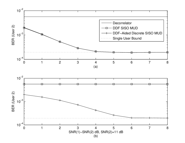
Figure 4: BER vs. SNR difference in two-user channel. (a) Strong user detected first. (b) Weak user detected first.

Consider an uncoded two-user synchronous CDMA system with spreading-sequence cross-correlation $\rho=0.7$. We let the signal-to-noise ratio (SNR) of user 1 (strong user) be no smaller than that of user 2 (weak user), i.e., $\mbox{SNR}(1)\geq\mbox{SNR}(2)$. Fixing $\mbox{SNR}(2)$ at $11$ dB and varying $\mbox{SNR}(1)$, we obtain the bit error rate (BER) of user 2 as shown in Fig. 4. In Fig. 4(a), we detect the strong user first. the DDF-aided discrete SISO MUD is implemented with the DDF SISO MUD followed by four discrete SISO MUD iterations. It is seen that in this case, the additional discrete SISO MUD iterations do not offer performance enhancement, thus the DDF-aided discrete SISO MUD performs nearly identical to DDF SISO MUD. The use of discrete SISO MUD alone suffers from poor convergence as predicted, and is omitted in the plot.

However, like Duel-Hallen’s conventional DDF detector, DDF SISO detector is sensitive to the detection order. This means if the weak user is detected first, the near-far resistance property no longer holds. Such an effect is depicted in Fig. 4(b), where we detect the weak user first. By fixing $\mbox{SNR}(2)$ at $11$ dB and varying $\mbox{SNR}(1)$, the BER of different schemes are plotted. It is seen that the DDF SISO MUD no longer approaches near-optimal performance as the SNR difference increases, while the DDF-aided discrete SISO MUD continues to demonstrate good near-far resistance even with non-optimal detection order. This is because the additional discrete SISO MUD iterations rectifies the performance degradation of DDF SISO MUD due to unfavourable detection order.

These simple examples reveal that the DDF-aided discrete SISO MUD is a much more powerful detection scheme compared to both discrete SISO MUD and DDF SISO MUD. It can be viewed as either the multiple-iteration extension to DDF SISO MUD, or as a discrete SISO MUD with convergence acceleration. The DDF-aided discrete SISO MUD is a powerful algorithm that is now capable of coping with strong-interference channels such as the ones assumed in [3], which will be studied in Section 6.

4.8 Summary

Table 3: Variational-inference-based multiuser detectors employing different scheduling schemes.

	Gaussian SISO	Discrete SISO
Sequential	$\star$	[31]
Flooding	$\star$	[2]
Hybrid	[3]	$\star$

Table 3 categorizes some of the existing turbo multiuser detectors according to the standard-form SISO MUD schemes outlined in Table 2 and 1. $\star$ indicates the schemes that are outcomes of the general framework, but not seen in the literature. We now outline how the existing schemes fit into the categories created.

• [3] is identical to the hybrid-Gaussian -SISO MUD, but it is re-derived in Section 4.4.1 via a completely different VFEM-based approach. With the help of the insights offered by the VFEM framework, we are able to further extend [3] to sequential and flooding schedule implementations, both explained in Section 4.4.2.

• [31] can be seen as the standard sequential-discrete-SISO MUD with sequential scheduling, and $I=1$ inner iteration. Moreover, [31] considers the joint estimation of noise-plus-MAI variance and channel amplitude. Like the noise-plus-MAI variance estimation in [2], this can also be studied within the VFEM framework, as an instance of the variational EM algorithm discussed in Section 5.

• [2] can be seen as a simplified version of flooding-discrete-SISO MUD, but it differs from the the standard approach in two aspects: 1) [2] uses parallel updates of each user’s bit LLR, which does not guarantee the reduction of free energy. 2) [2] uses the posterior estimate (instead of the extrinsic information) from the APP decoder as the initialization of $\mathbf{m}$, a practice that is suboptimal from the message-passing standpoint.

5 Variational EM for Iterative Parameter Estimation

In recent years, the impact of imperfect channel estimation on uncoded and coded multiuser detection have been studied in the large system limit [33, 34, 35]. However, the alleviation of this problem has rarely been systematically investigated in the literature. In this section, we will introduce an important extension of variational inference, called variational EM, to enable joint parameter estimation in turbo MUD. The two examples in Sections 5.2 and 5.3, based on the Gaussian SISO detector and discrete SISO detector, respectively, will illustrate how the variational EM framework provides a feasible solution to practical turbo receiver design when exact channel state information (CSI) is unavailable.

5.1 Formulation of Variational EM Algorithm

Like most detectors, variational-inference-based detection schemes assume perfect knowledge of system parameters, such as various types of channel information. These parameters, in practice however, may not be known accurately at the receiver. One traditional way to incorporate the uncertainties of these parameters in the detection operation is through the EM algorithm [36, 37]. The EM algorithm is used to estimate a vector of parameters, say $\boldsymbol{\theta}$, from the observation $\mathbf{r}$ that is termed “incomplete data”, together with some auxiliary or hidden variable, say $\mathbf{b}$. The algorithm iteratively carries out two operations: the E step and the M step. The $j$-th iteration effectively computes a probability density $p(\mathbf{b}|\mathbf{r},\boldsymbol{\theta}^{(j-1)})$ in the E step, where $\boldsymbol{\theta}^{(j-1)}$ is the estimate of $\boldsymbol{\theta}$ in the previous iteration, and then in the M step maximizes

$$U(\boldsymbol{\theta},\boldsymbol{\theta}^{(j-1)})=\int p(\mathbf{b}|\mathbf{r},\boldsymbol{\theta}^{(j-1)})\log p(\mathbf{b},\mathbf{r}|\boldsymbol{\theta})d\mathbf{b}$$ (65)

over $\boldsymbol{\theta}$, yielding $\boldsymbol{\theta}^{(j)}$.

The work in [15] shows that the EM algorithm is equivalent to jointly estimating the hidden variables and parameters by minimizing a single free-energy expression over a postulated distribution for the hidden variables, and over the parameters. The VFEM formulation offers an additional degree of freedom to the conventional EM algorithm, such that in the E step, an approximate posterior $Q(\mathbf{b}|\boldsymbol{\theta}^{(j-1)})$ may be used to replace the exact posterior $p(\mathbf{b}|\mathbf{r},\boldsymbol{\theta}^{(j-1)})$. Variational EM has been successfully applied in various applications, e.g., in image processing to perform scene analysis [38], and in joint detection/estimation problems in wireless channels [39, 40].

To provide a concrete example, assume $\boldsymbol{\theta}$ remains static over $T$ independent uses of the channel. In the context of MUD, this implies that we assume $\boldsymbol{\theta}$, the noise variance $\sigma^{2}$ for example, remains constant when a block of $T$ bits are transmitted by each user ($T$ could be the code word length). The variational EM algorithm extracts point estimates for $\boldsymbol{\theta}$ and postulated posterior distributions over the channel bits. Therefore, the new $Q$-function may be written as:

$$Q(\mathbf{b}_{1},\cdots,\mathbf{b}_{T},\boldsymbol{\theta})=\delta(\boldsymbol{\theta}-\hat{\boldsymbol{\theta}})\prod_{t=1}^{T}Q(\mathbf{b}_{t}),$$ (66)

where $\hat{\boldsymbol{\theta}}$ is an estimate of $\boldsymbol{\theta}$, and $\mathbf{b}_{t}$ contains the channel bits transmitted in the $t$-th use of the channel. The notation $\delta(\mathbf{a}-\hat{\mathbf{a}})$ denotes a vector Dirac delta function with the following properties: $\int\delta(\mathbf{a}-\hat{\mathbf{a}})f(\mathbf{a})\ d\mathbf{a}=f(\hat{\mathbf{a}})$, and $\int\delta(\mathbf{a}-\hat{\mathbf{a}})\ d\mathbf{a}=1$. Recall that for i.i.d. data, $p(\mathbf{b},\boldsymbol{\theta},\mathbf{r})=p(\boldsymbol{\theta})\prod_{t=1}^{T}p(\mathbf{b}_{t},\mathbf{r}_{t}|\boldsymbol{\theta})$. Substituting (66) into (10) yields the following free energy:

$$\begin{array}[]{rcl}\mathcal{F}&=&\displaystyle\int_{\mathbf{b}}\int_{\boldsymbol{\theta}}Q(\mathbf{b}_{1},\cdots,\mathbf{b}_{T},\boldsymbol{\theta})\log\frac{Q(\mathbf{b}_{1},\cdots,\mathbf{b}_{T},\boldsymbol{\theta})}{p(\mathbf{b}_{1},\cdots,\mathbf{b}_{T},\boldsymbol{\theta},\mathbf{r})}d\boldsymbol{\theta}d\mathbf{b}\\ &=&\displaystyle\int_{\mathbf{b}}\int_{\boldsymbol{\theta}}\delta(\boldsymbol{\theta}-\hat{\boldsymbol{\theta}})\prod_{t=1}^{T}Q(\mathbf{b}_{t})\log\frac{\delta(\boldsymbol{\theta}-\hat{\boldsymbol{\theta}})\prod_{t=1}^{T}Q(\mathbf{b}_{t})}{p(\boldsymbol{\theta})\prod_{t=1}^{T}p(\mathbf{b}_{t},\mathbf{r}_{t}|\boldsymbol{\theta})}d\boldsymbol{\theta}d\mathbf{b}\\ &=&\displaystyle\int_{\boldsymbol{\theta}}\delta(\boldsymbol{\theta}-\hat{\boldsymbol{\theta}})\log\delta(\boldsymbol{\theta}-\hat{\boldsymbol{\theta}})d\boldsymbol{\theta}-\int_{\boldsymbol{\theta}}\delta(\boldsymbol{\theta}-\hat{\boldsymbol{\theta}})\log p(\boldsymbol{\theta})d\boldsymbol{\theta}+\int_{\mathbf{b}}\prod_{t=1}^{T}Q(\mathbf{b}_{t})\log\frac{\prod_{t=1}^{T}Q(\mathbf{b}_{t})}{\prod_{t=1}^{T}p(\mathbf{b}_{t},\mathbf{r}_{t}|\hat{\boldsymbol{\theta}})}d\mathbf{b}\\ &=&\displaystyle-\log p(\hat{\boldsymbol{\theta}})+\sum_{t=1}^{T}\left(\int_{\mathbf{b}_{t}}Q(\mathbf{b}_{t})\log\frac{Q(\mathbf{b}_{t})}{p(\mathbf{b}_{t},\mathbf{r}_{t}|\hat{\boldsymbol{\theta}})}d\mathbf{b}_{t}\right).\end{array}$$ (67)

In the last line of the above equation we omit the constant term $\int_{\boldsymbol{\theta}}\delta(\boldsymbol{\theta}-\hat{\boldsymbol{\theta}})\log\delta(\boldsymbol{\theta}-\hat{\boldsymbol{\theta}})d\boldsymbol{\theta}$. The term $p(\hat{\boldsymbol{\theta}})$ constitutes the prior knowledge of the parameter. In cases when it is not available, we may set $p(\hat{\boldsymbol{\theta}})=constant$ and ignore it in the minimization of free energy.

As proven in [15], alternating between minimizing (67) w.r.t. $\{Q(\mathbf{b}_{t})\}_{t=1}^{T}$ in the E step, and w.r.t. $\hat{\boldsymbol{\theta}}$ in the M Step leads to the exact EM algorithm where $\{\mathbf{b}_{t}\}_{t=1}^{T}$ are the “hidden variables” and $\hat{\boldsymbol{\theta}}$ is the unknown parameter of interest. Unfortunately, the exact EM is only possible in special cases, because the computation in the E step of $Q(\mathbf{b}_{t})=p(\mathbf{b}_{t}|\mathbf{r}_{t},\hat{\boldsymbol{\theta}})$ (s.t. $\int_{\mathbf{b}_{t}}Q(\mathbf{b}_{t})d\mathbf{b}_{t}=1$) is often intractable. But suppose we use a postulated (and simple) distribution $Q(\mathbf{b}_{t})$, with parameter $\lambda_{t}$, and then find $\lambda_{t}$ that minimizes (67). We then arrive at the variational EM algorithm, which consists of the initialization plus the E step and M step in the $j$-th iteration:

Initialization Choose initial values for $\hat{\boldsymbol{\theta}}^{(0)}$. E Step Minimize $\mathcal{F}(\lambda_{1},\cdots,\lambda_{T},\hat{\boldsymbol{\theta}}^{(j-1)})$ in (67) w.r.t. $\lambda_{t}$ $$\lambda_{t}^{(j)}=\arg\min_{\lambda_{t}}\int_{\mathbf{b}_{t}}Q(\mathbf{b}_{t})\log\frac{Q(\mathbf{b}_{t})}{p(\mathbf{b}_{t},\mathbf{r}_{t}|\hat{\boldsymbol{\theta}}^{(j-1)})}d\mathbf{b}_{t},$$ (68) for $t=1,\cdots,T$. M Step Minimize $\mathcal{F}(\lambda_{1}^{(j)},\cdots,\lambda_{T}^{(j)},\hat{\boldsymbol{\theta}})$ in (67) w.r.t. $\hat{\boldsymbol{\theta}}$ $$\hat{\boldsymbol{\theta}}^{(j)}=\arg\min_{\hat{\boldsymbol{\theta}}}\sum_{t=1}^{T}\left(\int_{\mathbf{b}_{t}}Q^{(j)}(\mathbf{b}_{t})\log\frac{Q^{(j)}(\mathbf{b}_{t})}{p(\mathbf{b}_{t},\mathbf{r}_{t}|\hat{\boldsymbol{\theta}})}d\mathbf{b}_{t}\right)-\log p(\hat{\boldsymbol{\theta}}).$$ (69)

In the rest of the section, we will implement the variational EM algorithm in both Gaussian SISO MUD and discrete SISO MUD, to resolve the uncertainty in channel information at the receiver. More specifically, we will assume no noise variance information and noisy channel amplitude information at the receiver, and attempt to adaptively estimate the noise variance, as well as improve the channel amplitude estimation, jointly with data detection.

5.2 Channel and Noise Variance Estimation for Gaussian SISO MUD

Adding a time index $t$ to (1) to represent a sequence of channel observations $\mathbf{r}_{t}=\mathbf{S}\mathbf{A}\mathbf{b}_{t}+\mathbf{n}_{t}$ ($t=1,\cdots,T$), according to (67), we may write the free energy for $T$ channel realizations as

$$\mathcal{F}_{gauss}(\boldsymbol{\mu}_{1},\cdots,\boldsymbol{\mu}_{T},\mathbf{\Sigma}_{1},\cdots,\mathbf{\Sigma}_{T},\sigma^{2},\mathbf{a})=-\log p(\sigma^{2})-\log p(\mathbf{a})+\sum_{t=1}^{T}\mathcal{F}_{gauss}(\boldsymbol{\mu}_{t},\mathbf{\Sigma}_{t}|\sigma^{2},\mathbf{a}).$$ (70)

where $\mathbf{a}=\mathop{\sf diag}(\mathbf{A})$, and we define

$$\mathcal{F}_{gauss}(\boldsymbol{\mu}_{t},\mathbf{\Sigma}_{t}|\sigma^{2},\mathbf{a})=\int_{\mathbf{b}_{t}}Q(\mathbf{b}_{t})\log\frac{Q(\mathbf{b}_{t})}{p(\mathbf{b}_{t},\mathbf{r}_{t}|\sigma^{2},\mathbf{a})}d\mathbf{b}_{t},$$ (71)

which is equal to (29), except that $\sigma^{2}$ and $\mathbf{a}$ are now explicitly shown to be variables of $\mathcal{F}$. Here $\boldsymbol{\theta}=\{\sigma^{2},\mathbf{a}\}$ are the model parameters to be estimated. In (70), $p(\sigma^{2})$ is a constant, since we do not assume prior knowledge about $\sigma^{2}$. But estimates of the channel, however noisy, can be assumed available at the receiver. In particular, we model the true channel, $\mathbf{a}$, as the sum of the channel estimate, $\tilde{\mathbf{a}}$, and random measurement error with variance $\varsigma^{2}$ [41]. Or, equivalently, $p(\mathbf{a})=\mathcal{N}(\tilde{\mathbf{a}},\varsigma^{2}\mathbf{I})$, where $\varsigma$ is assumed to be known.

The E step, i.e., the estimation of $\boldsymbol{\mu}$ and $\mathbf{\Sigma}$, has already been completed in Section 4.4. The only challenge now remaining is the M step. From (69), we see that we are required to solve for

$$\{\hat{\sigma}^{2},\hat{\mathbf{a}}\}=\arg\min_{\sigma^{2},\mathbf{a}}\ \mathcal{F}_{gauss}(\boldsymbol{\mu}_{1},\cdots,\boldsymbol{\mu}_{T},\mathbf{\Sigma}_{1},\cdots,\mathbf{\Sigma}_{T},\sigma^{2},\mathbf{a}).$$ (72)

To this end, the following identity is needed:

Lemma 1

$$\mathop{\sf tr}[\mathop{\sf diag}(\mathbf{x})\cdot\mathbf{A}\cdot\mathop{\sf diag}(\mathbf{y})\cdot\mathbf{B}]=\mathbf{x}^{T}(\mathbf{A}\circ\mathbf{B}^{T})\mathbf{y}$$ (73)

for square matrices $\mathbf{A}$, $\mathbf{B}\in\mathbb{R}^{N\times N}$, and vectors $\mathbf{x}$, $\mathbf{y}\in\mathbb{R}^{N\times 1}$.

Proof: Writing $\mathbf{A}=[A_{ij}]$ and $\mathbf{B}=[B_{ij}]$, it is easily verified that both sides of the equation are equal to $\sum_{i,j}x_{i}A_{ij}B_{ji}y_{j}$.   

Utilizing Lemma 1 and ignoring the terms independent of $\sigma^{2}$ and $\mathbf{a}$, we have

$$\begin{array}[]{rl}&\mathcal{F}_{gauss}(\boldsymbol{\mu}_{1},\cdots,\boldsymbol{\mu}_{T},\mathbf{\Sigma}_{1},\cdots,\mathbf{\Sigma}_{T},\sigma^{2},\mathbf{a})\\ =&\sum_{t=1}^{T}\left\{\frac{1}{2\sigma^{2}}(\mathbf{r}_{t}-\mathbf{S}\mathbf{\mathcal{M}}_{t}\mathbf{a})^{T}(\mathbf{r}_{t}-\mathbf{S}\mathbf{\mathcal{M}}_{t}\mathbf{a})+\frac{N}{2}\log(\sigma^{2})+\frac{1}{2\sigma^{2}}\mathbf{a}^{T}[(\mathbf{S}^{T}\mathbf{S})\circ\mathbf{\Sigma}_{t}]\mathbf{a}+\frac{1}{2\varsigma^{2}}(\mathbf{a}-\tilde{\mathbf{a}})^{T}(\mathbf{a}-\tilde{\mathbf{a}})\right\},\end{array}$$ (74)

where $\mathbf{\mathcal{M}}_{t}=\mathop{\sf diag}(\boldsymbol{\mu}_{t})$. Equating $\partial\mathcal{F}/\partial\mathbf{a}=\mathbf{0}$ produces

$$\hat{\mathbf{a}}=\left\{\sum_{t=1}^{T}\mathbf{\mathcal{M}}_{t}^{T}\mathbf{S}^{T}\mathbf{S}\mathbf{\mathcal{M}}_{t}+(\mathbf{S}^{T}\mathbf{S})\circ\mathbf{\Sigma}_{t}+\frac{\sigma^{2}}{\varsigma^{2}}\mathbf{I}\right\}^{-1}\left(\sum_{t=1}^{T}\mathbf{\mathcal{M}}_{t}\mathbf{S}^{T}\mathbf{r}_{t}+\frac{\sigma^{2}}{\varsigma^{2}}\tilde{\mathbf{a}}\right).$$ (75)

Substituting $\mathbf{a}=\hat{\mathbf{a}}$ into $\mathcal{F}$ and solving for $\mathcal{F}(\boldsymbol{\mu}_{1},\cdots,\boldsymbol{\mu}_{T},\mathbf{\Sigma}_{1},\cdots,\mathbf{\Sigma}_{T},\sigma^{2},\hat{\mathbf{a}})/\partial\sigma^{-2}=0$ gives

$$\hat{\sigma}^{2}=\frac{1}{NT}\left\{\sum_{t=1}^{T}\left[(\mathbf{r}_{t}-\mathbf{S}\hat{\mathbf{A}}\boldsymbol{\mu}_{t})^{T}(\mathbf{r}_{t}-\mathbf{S}\hat{\mathbf{A}}\boldsymbol{\mu}_{t})+\hat{\mathbf{a}}^{T}[(\mathbf{S}^{T}\mathbf{S})\circ\mathbf{\Sigma}_{t}]\hat{\mathbf{a}}\right]\right\},$$ (76)

where $\hat{\mathbf{A}}=\mathop{\sf diag}(\hat{\mathbf{a}})$. Note that (75) and (76) decrease the free energy in a coordinate descent manner, not necessarily minimizing it, due to the coupling of $\mathbf{a}$ and $\sigma^{2}$ in the two equations. But this is acceptable, since they will converge to the exact minimizers over the EM iterations.

After incorporating iterative decoding, the variational EM algorithm for turbo MUD employing flooding-Gaussian-SISO MUD is described in Table 4.

Table 4: Variational EM algorithm employing Gaussian SISO MUD.

Initialization	Set $\tilde{\mathbf{b}}_{t}=\mathbf{0}$, $\sigma^{2(0)}=0$, and $\mathbf{a}^{(0)}=\tilde{\mathbf{a}}$.
Update for $Q(\mathbf{b})$ E Step	FOR $j=1:J$ (Outer Iteration) FOR $k=1:K$ and $t=1:T$ $\tilde{\mathbf{b}}_{t,k}$ = $[\tilde{b}_{t,1},\cdots,\tilde{b}_{t,k-1},0,\tilde{b}_{t,k+1},\cdots,\tilde{b}_{t,K}]^{T}$ $\mathbf{W}_{t}$ = $\mathop{\sf diag}([1-\tilde{b}_{t,1}^{2},\cdots,1-\tilde{b}_{t,K}^{2}]^{T})$ $\check{\mu}_{t,k}$ = $A_{k}\mathbf{e}_{k}^{T}\left[\mathbf{A}^{T}\mathbf{W}_{t}\mathbf{A}+\sigma^{2}\mathbf{R}^{-1}\right]^{-1}\left[\mathbf{R}^{-1}\mathbf{y}_{t}-\mathbf{A}\tilde{\mathbf{b}}_{t,k}\right]$ $\check{\alpha}_{t,k}$ = $(1-\tilde{b}_{t,k}^{2})A_{k}^{2}\left[(\mathbf{A}^{T}\mathbf{W}_{t}\mathbf{A}+\sigma^{2}\mathbf{R}^{-1})^{-1}\right]_{k,k}$ $\mbox{LLR}_{mud}(b_{t,k})=\frac{2\check{\mu}_{t,k}}{1-\check{\alpha}_{t,k}}$ END
BCJR Decoding	FOR $k=1:K$ and $t=1:T$ $\mbox{LLR}_{dec}(b_{t,k})\stackrel{{\scriptstyle\scriptsize\mbox{Decoding}}}{{\Longleftarrow}}\mbox{LLR}_{mud}(b_{t,k})$   (Extrinsic Information) $\tilde{b}_{t,k}$ = $\tanh[\mbox{LLR}_{dec}(b_{t,k})/2]$ $\hat{b}_{t,k}$ = $\tanh[\mbox{LLR}_{mud}(b_{t,k})/2+\mbox{LLR}_{dec}(b_{t,k})/2]$ (Posterior Estimate) $\mu_{t,k}$ $\leftarrow$ $\hat{b}_{t,k}$ $[\mathbf{\Sigma}_{t}]_{k,k}\leftarrow 1-\mu_{t,k}^{2}$ END
Update for $\sigma^{2}$ and $\mathbf{a}$ M Step	$\mathbf{a}$ $\leftarrow$ $\left\{\sum_{t=1}^{T}\mathbf{\mathcal{M}}_{t}^{T}\mathbf{S}^{T}\mathbf{S}\mathbf{\mathcal{M}}_{t}^{T}+(\mathbf{S}^{T}\mathbf{S})\circ\mathbf{\Sigma}_{t}+\frac{\sigma^{2}}{\varsigma^{2}}\mathbf{I}\right\}^{-1}\left(\sum_{t=1}^{T}\mathbf{\mathcal{M}}_{t}\mathbf{S}^{T}\mathbf{r}_{t}+\frac{\sigma^{2}}{\varsigma^{2}}\tilde{\mathbf{a}}\right)$ $\sigma^{2}$ $\leftarrow$ $\frac{1}{NT}\left\{\sum_{t=1}^{T}\left[(\mathbf{r}_{t}-\mathbf{S}\mathbf{A}\boldsymbol{\mu}_{t})^{T}(\mathbf{r}_{t}-\mathbf{S}\mathbf{A}\boldsymbol{\mu}_{t})+\mathbf{a}^{T}[(\mathbf{S}^{T}\mathbf{S})\circ\mathbf{\Sigma}_{t}]\mathbf{a}\right]\right\}$
	END

This is an extension to the flooding-Gaussian-SISO MUD algorithm in Table 1. The variational EM extension to sequential or hybrid Gaussian-SISO MUD is straightforward, where the M step may be implemented either once every outer iteration $j$, or more frequently, after the E step update of each user.

5.3 Channel and Noise Variance Estimation for Discrete SISO MUD

Similar to Gaussian SISO MUD, the free energy of discrete SISO MUD for $T$ channel outputs can be written as

$$\mathcal{F}_{disc}(\mathbf{m}_{1},\cdots,\mathbf{m}_{T},\sigma^{2},\mathbf{a})=-\log p(\sigma^{2})-\log p(\mathbf{a})+\sum_{t=1}^{T}\mathcal{F}_{disc}(\mathbf{m}_{t}|\sigma^{2},\mathbf{a}),$$ (77)

$\mathcal{F}_{disc}(\mathbf{m}_{t}|\sigma^{2},\mathbf{a})$ is simply (46) with an additional time index $t$. In (77), we set $p(\sigma^{2})$ to a constant and let $p(\mathbf{a})=\mathcal{N}(\tilde{\mathbf{a}},\varsigma^{2}\mathbf{I})$. Making use of the E step already derived in Section 4.5, we only need to complete the M step.

Utilizing Lemma 1 and ignoring the terms independent of $\sigma^{2}$ and $\mathbf{a}$, we have

$$\begin{array}[]{rl}&\mathcal{F}_{disc}(\mathbf{m}_{1},\cdots,\mathbf{m}_{T},\sigma^{2},\mathbf{a})\\ =&\sum_{t=1}^{T}\left\{\frac{N}{2}\log(\sigma^{2})+\frac{1}{2\sigma^{2}}\mathbf{a}^{T}[\mathbf{M}_{t}^{T}\mathbf{S}^{T}\mathbf{S}\mathbf{M}_{t}-\mathop{\sf diag}(\mathbf{M}_{t}^{T}\mathbf{S}^{T}\mathbf{S}\mathbf{M}_{t})]\mathbf{a}+\frac{1}{2\sigma^{2}}\mathbf{a}^{T}\mathop{\sf diag}(\mathbf{S}^{T}\mathbf{S})\mathbf{a}-\frac{1}{\sigma^{2}}\mathbf{r}_{t}^{T}\mathbf{S}\mathbf{M}_{t}\mathbf{a}\right\}\\ &+\frac{1}{2\varsigma^{2}}(\mathbf{a}-\tilde{\mathbf{a}})^{T}(\mathbf{a}-\tilde{\mathbf{a}}),\end{array}$$ (78)

where $\mathbf{M}_{t}=\mathop{\sf diag}(\mathbf{m}_{t})$. Equating $\partial\mathcal{F}/\partial\mathbf{a}=\mathbf{0}$ produces

$$\textstyle\hat{\mathbf{a}}=\left\{\sum_{t=1}^{T}\mathop{\sf diag}(\mathbf{S}^{T}\mathbf{S})+\mathbf{M}_{t}^{T}[\mathbf{S}^{T}\mathbf{S}-\mathop{\sf diag}(\mathbf{S}^{T}\mathbf{S})]\mathbf{M}_{t}\right\}^{-1}\left(\sum_{t=1}^{T}\mathbf{M}_{t}\mathbf{S}^{T}\mathbf{r}_{t}+\frac{\sigma^{2}}{\varsigma^{2}}\tilde{\mathbf{a}}\right).$$ (79)

Substituting $\mathbf{a}=\hat{\mathbf{a}}$ into $\mathcal{F}$ and solve for $\mathcal{F}(\mathbf{m}_{1},\cdots,\mathbf{m}_{T},\sigma^{2},\hat{\mathbf{a}})/\partial\sigma^{-2}=0$ gives

$$\hat{\sigma}^{2}=\frac{1}{NT}\left\{\sum_{t=1}^{T}\left[(\mathbf{r}_{t}-\mathbf{S}\hat{\mathbf{A}}\mathbf{m}_{t})^{T}(\mathbf{r}_{t}-\mathbf{S}\hat{\mathbf{A}}\mathbf{m}_{t})+\sum_{k=1}^{K}(1-m_{t,k}^{2})\hat{A}_{k}^{2}\cdot\mathbf{s}_{k}^{T}\mathbf{s}\right]\right\}.$$ (80)

The variational EM algorithm for flooding-discrete-SISO MUD is presented in Table 5.

Table 5: Variational EM algorithm employing Discrete SISO MUD.

Initialization	Set $\tilde{\mathbf{m}}_{t}=\mathbf{0}$, $\mbox{LLR}_{dec}(b_{t,k}=0)$, $\sigma^{2(0)}=0$, and $\mathbf{a}^{(0)}=\tilde{\mathbf{a}}$.
Update for $Q(\mathbf{b})$ E Step	FOR $j=1:J$ (Outer Iteration) FOR $i=1:I$ (Inner Iteration) FOR $k=1:K$ and $t=1:T$ $\mbox{LLR}_{pos}(b_{t,k})=\mbox{LLR}_{dec}(b_{t,k})+\frac{2}{\sigma^{2}}\left[\boldsymbol{\eta}_{k}^{T}\mathbf{r}_{t}-\boldsymbol{\beta}_{k}^{T}\mathbf{m}_{t}\right]$ $m_{t,k}=\tanh[\mbox{LLR}_{pos}(b_{t,k})/2]$ END END
BCJR Decoding	FOR $k=1:K$ and $t=1:T$ $\mbox{LLR}_{mud}(b_{t,k})=\mbox{LLR}_{pos}(b_{t,k})-\mbox{LLR}_{dec}(b_{t,k})$ $\mbox{LLR}_{dec}(b_{t,k})\stackrel{{\scriptstyle\scriptsize\mbox{Decoding}}}{{\Longleftarrow}}\mbox{LLR}_{mud}(b_{t,k})$   (Extrinsic Information) $\hat{b}_{t,k}$ = $\tanh[\mbox{LLR}_{mud}(b_{t,k})/2+\mbox{LLR}_{dec}(b_{t,k})/2]$ (Posterior Estimate) $m_{t,k}$ $\leftarrow$ $\hat{b}_{t,k}$ END
Update for $\sigma^{2}$ and $\mathbf{a}$ M Step	$\mathbf{a}$ $\leftarrow$ $\left\{\sum_{t=1}^{T}\mathbf{S}^{T}\mathbf{S}+\mathbf{M}_{t}^{T}[\mathbf{S}^{T}\mathbf{S}-\mathop{\sf diag}(\mathbf{S}^{T}\mathbf{S})]\mathbf{M}_{t}+\frac{\sigma^{2}}{\varsigma^{2}}\mathbf{I}\right\}^{-1}\left(\sum_{t=1}^{T}\mathbf{M}_{t}\mathbf{S}^{T}\mathbf{r}_{t}+\frac{\sigma^{2}}{\varsigma^{2}}\tilde{\mathbf{a}}\right)$ $\sigma^{2}$ $\leftarrow$ $\frac{1}{NT}\left\{\sum_{t=1}^{T}\left[(\mathbf{r}_{t}-\mathbf{S}\mathbf{A}\mathbf{m}_{t})^{T}(\mathbf{r}_{t}-\mathbf{S}\mathbf{A}\mathbf{m}_{t})-\sum_{k=1}^{K}(1-m_{t,k}^{2})A_{k}^{2}\cdot\mathbf{s}_{k}^{T}\mathbf{s}_{k}\right]\right\}$
	END

Now consider taking a step backward and assume $\mathbf{a}$ to be known perfectly, and only $\sigma^{2}$ needs to be estimated. It is clear that, in (80), each element of $\mathbf{m}_{t}$ converges to $-1$ or $+1$ as the algorithm converges. Hence, the last term in (80) eventually vanishes. By omitting the vanishing term, this is exactly the equation to estimate $\sigma_{tot}^{2}=\sigma^{2}+\sigma_{MU}^{2}$ in [2]. Together with Section 4.5, we have now completed the interpretation of Alexander-Grant-Reed’s turbo detector as an instance of the variational EM algorithm.

6 Simulation Results

In this section, we investigate the performance of turbo multiuser detectors employing the Gaussian SISO MUD and DDF-aided discrete SISO MUD (the original-form discrete SISO MUD would suffer from poor convergence due to the non-convexity of $\mathcal{F}_{disc}(\mathbf{m})$). We will consider two different scenarios to test the proposed schemes in both standard benchmark settings and in more practical situations:

Scenario I:

A flat-fading synchronous CDMA channel same as that in [3]: A four-user system is assumed with equal cross-correlation $\rho=0.7$. All users have equal power and employ the same rate $1/2$ convolutional code with generators $10011$ and $11101$.

Scenario II:

A flat-fading synchronous CDMA channel with random spreading: The system has spreading gain of $N=32$ and $K=32$ active users. All users have equal power and employ the same rate $1/2$ convolutional code with generators $111$ and $101$. In this case, we also assume the receiver has noisy channel information (unknown $\sigma^{2}$ and inaccurate channel amplitude estimates).

Since the focus of this paper is the introduction of a theoretical framework, these test results are for proof-of-concept purposes only and are by no means complete. More elaborate and complete simulations, such as the near-far situation or the extensions to multipath channels, may be performed following the same recipe presented in [3] and will be omitted.

6.1 Gaussian SISO MUD

6.1.1 Scenario I with Perfect Channel Knowledge

In Section 4.4.2, we proved that the Wang-Poor turbo MUD scheme is an instance of hybrid-Gaussian-SISO MUD, whose performance is depicted in Fig. 3 of [3]. In this paper, we will realize the other two variations, namely sequential-Gaussian-SISO MUD and flooding-Gaussian-SISO MUD, predicted by the theory of VFEM and the associated message passing rules. The complete Gaussian SISO MUD algorithms are described in Table 1.

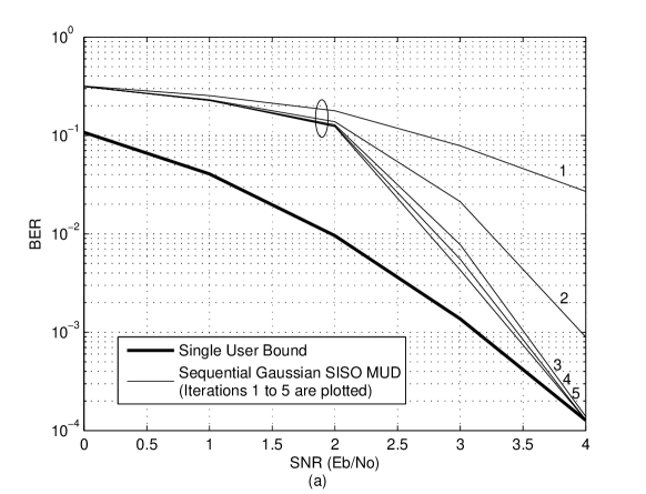
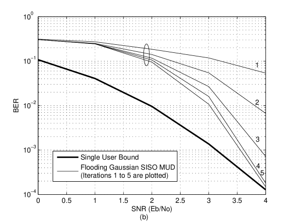
Figure 5: BER performance of turbo MUD employing Gaussian-SISO MUD ($K=4$, $\rho=0.7$). (a) Sequential schedule; (b) Flooding schedule.

Fig. 5(a) and Fig. 5(b) plot the BER performance of turbo MUD employing sequential-Gaussian-SISO MUD and flooding-Gaussian-SISO MUD, respectively, in simulation scenario I. The results after each of the $J=5$ outer iterations are recorded. It is shown that both schemes out-perform hybrid-Gaussian-SISO MUD, which was originally proposed outside of the variational inference framework. The BER improvement, although small, verifies that the sequential and flooding scheduling schemes are sound in practice as they are in theory.

In the above simulations, we find that the difference in performance between sequential schedule and flooding schedule is small. For conciseness, in the case of inaccurate channel estimates, we will only consider the flooding schedule, since it in general leads to lower overall complexity and latency at both the detection and decoding stages. That been said, one may choose to implement the sequential or hybrid schedule with ease as special need arises.

6.1.2 Scenario II with Unknown Noise Variance and Inaccurate Channel Estimates

We now consider simulation scenario II, a more challenging situation where the receiver is assumed to have no noise variance information and only inaccurate channel estimates. The actual channel is assumed to be Gaussian-distributed conditioned on the inaccurate estimate $\tilde{\mathbf{a}}$, i.e., $p(\mathbf{a})=\mathcal{N}(\tilde{\mathbf{a}},\varsigma^{2}\mathbf{I})$, as in Section 5.2. In the simulations, we fix the true channel $A_{k}=1$ (or $\mathbf{a}=\mathbf{1}$), and generate the noisy channel estimate $\tilde{A}_{k}$ as $1+\delta_{k}$, where $p(\delta_{k})=\mathcal{N}(0,\varsigma^{2})$.

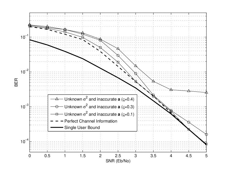
Figure 6: BER performance of turbo MUD employing flooding-Gaussian-SISO MUD with joint noise variance and channel estimation ($N=32$, $K=32$). The single user bound is obtained by assuming perfect channel knowledge.

Fig. 6 depicts the flooding-Gaussian-SISO MUD implemented with joint $\mathbf{a}$ and $\sigma^{2}$ estimation. We set $\varsigma$ to be $0.1$, $0.3$ and $0.4$, respectively, to be compared with the case of exact channel knowledge at the receiver. To be consistent, the curves plotted are the results after $J=10$ outer iterations, although in most cases convergence is achieved with fewer iterations. It is seen that, with the help of the variational EM algorithm, this turbo multiuser detector is very robust to severe channel estimation error, up to $\varsigma=0.3$. It is only when $\varsigma$ reaches $0.4$, i.e., $40\%$ that of the actual channel amplitude, significant performance degradation starts to appear.

6.2 DDF-Aided Discrete SISO MUD

6.2.1 Scenario I with Unknown Noise Variance Only

To implement DDF-aided discrete SISO MUD in turbo MUD, we simply need to replace the first outer iteration ($j=1$) in the algorithms of Table 2 with DDF update (63), and keep the remaining outer iterations ($j\geq 2$) the same. We will first simulate scenario I with turbo MUD employing DDF-aided sequential-discrete-SISO MUD and DDF-aided flooding-discrete-SISO MUD, each having $I=6$ inner iterations within every outer iteration, except for the first outer iteration, where the DDF update only requires $1$ inner iteration. In the detection algorithms prescribed in Table 2, we added a noise variance estimate step like it is done in [2, 31]. This is a special case of the variational EM algorithm introduced in Section 5.3 with $\sigma^{2}$ alone being the unknown parameter. Having the noise variance as an unknown does not seem to temper the detector performance compared to perfectly-known noise variance, and, in certain cases, even helps. We attribute this phenomenon to its possible relation with optimizing (46) via simulation annealing by setting $\sigma^{2}$ to be the temperature parameter [42], but will leave detailed discussions to future works.

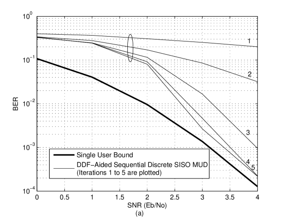
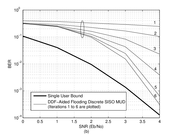
Figure 7: BER performance of turbo MUD employing discrete-SISO MUD with joint noise variance estimation ($K=4$, $\rho=0.7$). (a) Sequential schedule; (b) Flooding schedule.

Fig. 7(a) and Fig. 7(b) depict the BER performance of the above-mentioned schemes over $J=5$ or $6$ outer iteration. Despite the slightly inferior performance compared to the Gaussian SISO counterparts, the DDF-aided discrete SISO detectors have been shown to produce excellent results even with unknown noise variance. The existing discrete SISO detectors, such as [2, 31], would fail under such simulation settings, due to the lack of DDF initialization.

6.2.2 Scenario II with Unknown Noise Variance and Inaccurate Channel Estimates

We now further investigate the case of inaccurate channel estimates in addition to unknown noise variance with simulation scenario II. Like the Gaussian SISO case, we set the true channel to be $A_{k}=1$, and generate noisy channel estimates by letting $\tilde{A}_{k}$ be $1+\delta_{k}$, where $p(\delta_{k})=\mathcal{N}(0,\varsigma^{2})$.

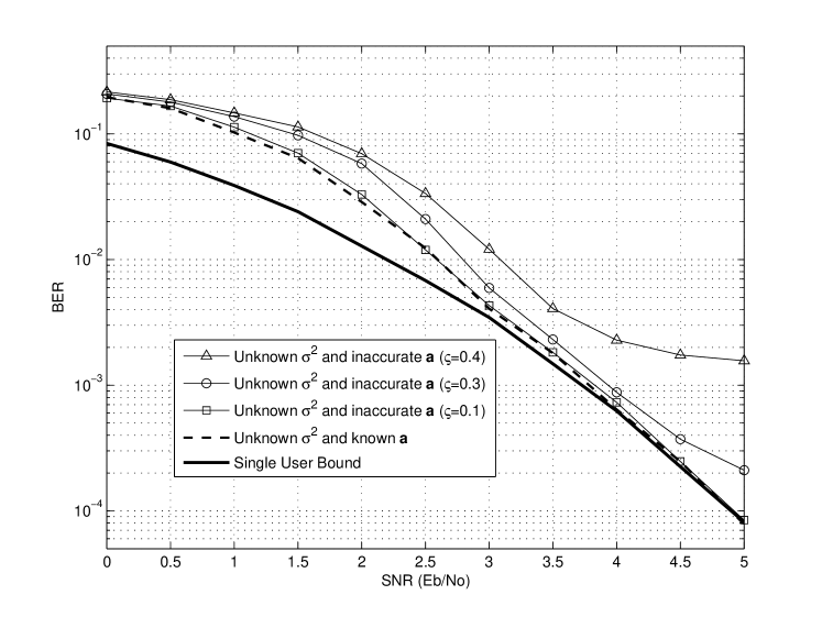
Figure 8: BER performance of turbo MUD employing flooding-discrete-SISO MUD with joint noise variance and channel estimation ($N=32$, $K=32$). The single user bound is obtained by assuming perfect channel knowledge.

Fig. 8 depicts the performance of DDF-aided flooding-discrete-SISO MUD under channel estimation error of $\varsigma=0.1$, $0.3$ and $0.4$, respectively. It is shown that, by iteratively refining the channel estimates, the modified flooding-discrete-SISO MUD is also robust to significant errors in channel estimation.

7 Conclusions

The concept of free energy is a far-reaching one. Besides its original formulation in statistical physics, it also recently finds its application in interpreting various probabilistic inference techniques, such as the EM algorithm [15] and belief propagation (sum-product algorithm) [43].

The main focus of this paper is the introduction of a comprehensive theory, centered around the minimization of variational free energy, that would describe various SISO detectors in multiple access channels. In particular, we developed guidelines for SISO detector design in linear Gaussian vector channels, first by pointing out the importance of message-passing scheduling, and next by deriving detection algorithms accordingly. We show that it is a carefully-chosen scheduling scheme combined with its accompanying SISO detector that produces a good turbo detector, opposed to the conventional view that focuses on the detector design alone. With this new paradigm comes a spectrum of plausible SISO detectors. In addition to new detectors constructed as a result, we show that some of the classic SISO detectors can be seen as special instances of this composition, and subsequently refined systematically.

In the algorithm design stage, after the postulation of prior and posterior distributions with the help of some intuition, it may be seen that our efforts in obtaining good algorithms have been condensed to the evaluation and optimization of free energy expressions, such as the ones at the centre of this paper, $\mathcal{F}_{gauss}(\boldsymbol{\mu},\mathbf{\Sigma})$ and $\mathcal{F}_{disc}(\mathbf{m})$. By viewing existing MUD schemes under the same roof, we obtain many interesting insights. Furthermore, we extended the initiative to variational-EM-based MUD, in which channel parameters may be efficiently and blindly estimated in conjunction with turbo MUD.

References

• [1] C. Berrou, A. Glavieux, and P. Titmajshima, “Near Shannon limit error-correction coding and decoding: Turbo codes,” in Proc. IEEE Int. Conf. Commun. (ICC’93), May 1993, pp. 1064–1070.
• [2] P. D. Alexander, A. J. Grant, and M. C. Reed, “Iterative detection in code-division multiple-access with error control coding,” Euro. Trans. Telecommun., vol. 9, no. 5, pp. 419–426, Oct. 1998.
• [3] X. Wang and H. V. Poor, “Iterative (turbo) soft interference cancellation and decoding for coded CDMA,” IEEE Trans. Commun., vol. 47, no. 7, pp. 1046–1061, July 1999.
• [4] C. Douillard, A. Picart, P. Didier, M. Jézéquel, C. Berrou, and A. Glavieux, “Iterative correction of intersymbol interference: Turbo equalization,” Euro. Trans. Telecommun., vol. 6, pp. 507–511, Sept. 1995.
• [5] M. Tüchler, A. C. Singer, and R. Koetter, “Turbo equalization: Principles and new results,” IEEE Trans. Commun., vol. 50, no. 5, pp. 754–767, May 2002.
• [6] S. L. Ariyavisitakul, “Turbo space-time processing to improve wireless channel capacity,” IEEE Trans. Commun., vol. 48, no. 8, pp. 1347–1359, Aug. 2000.
• [7] S. Haykin, M. Sellathurai, Y. de Jong, and T. Willink, “Turbo-MIMO for wireless communications,” IEEE Commun. Mag., vol. 42, no. 10, pp. 48–53, Oct. 2004.
• [8] S. Verdù, Multiuser Detection.   Cambridge, U.K.: Cambridge University Press, 1998.
• [9] L. Bahl, J. Cocke, F. Jelinek, and J. Raviv, “Optimal decoding of linear codes for minimizing symbol error rate,” IEEE Trans. Inf. Theory, vol. IT-20, pp. 284–287, Mar. 1974.
• [10] D. MacKay, Information Theory, Inference and Learning Algorithms.   Cambridge U.K.: Cambridge University Press, 2003.
• [11] F. R. Kschischang, B. J. Frey, and H. A. Loeliger, “Factor graphs and the sum-product algorithm,” IEEE Trans. Inf. Theory, vol. 47, no. 2, pp. 498–519, Feb. 2001.
• [12] J. Boutros and G. Caire, “Iterative multiuser joint decoding: Unified framework and asymptotic analysis,” IEEE Trans. Inf. Theory, vol. 48, no. 7, pp. 1772–1793, July 2002.
• [13] T. Tanaka, “A statistical-mechanics approach to large-system analysis of CDMA multiuser detectors,” IEEE Trans. Inf. Theory, vol. 48, no. 11, pp. 2888–2910, Nov. 2002.
• [14] D. Guo and S. Verdú, “Randomly spread CDMA: Asymptotics via statistical physics,” IEEE Trans. Inf. Theory, vol. 51, no. 6, pp. 1983–2010, June 2005.
• [15] R. M. Neal and G. E. Hinton, “A view of the EM algorithm that justifies incremental, sparse, and other variants,” in Learning in Graphical Models, M. I. Jordan, Ed.   Kluwer Academic Publishers, 1998.
• [16] D. D. Lin and T. J. Lim, “Multiuser detection of $M$-QAM symbols via bit-level equalization and soft detection,” in Proc. IEEE Int. Symp. Information Theory (ISIT’06), July 2006, pp. 1909–1913.
• [17] ——, “Turbo equalization for Gray-coded m-ary QAM with bit-level soft decisions,” in Proc. IEEE Int. Symp. Information Theory (ISIT’07), June 2007, pp. 1701–1705.
• [18] F. R. Kschischang and B. J. Frey, “Iterative decoding of compound codes by probability propagation in graphical models,” IEEE J. Sel. Areas Commun., vol. 16, no. 2, pp. 219–230, Feb. 1998.
• [19] N. Yacov, H. Efraim, H. Kfir, I. Kanter, and O. Shental, “Parallel vs. sequential belief propagation decoding of LDPC codes over ${GF}(q)$ and Markov sources,” Physica A: Statistical Mechanics and Its Applications, vol. 378, no. 2, pp. 329–335, May 2007.
• [20] M. I. Jordan, An Introduction to Probabilistic Graphical Models.   In Preparation.
• [21] B. J. Frey, Graphical Models for Machine Learning and Digital Communication.   Cambridge, Massachusetts: MIT Press, 1998.
• [22] M. I. Jordan, Z. Ghahramani, T. Jaakkola, and L. K. Saul, “An introduction to variational methods for graphical models,” Machine Learning, vol. 37, no. 2, pp. 183–233, 1999.
• [23] R. K. Pathria, Statistical Mechanics.   Oxford: Elsevier Butterworth-Heinemann, 2004.
• [24] H. Elders-Boll, H. D. Schotten, and A. Busboom, “Efficient implementation of linear multiuser detectors for asynchronous CDMA systems by linear interference cancellation,” Euro. Trans. Telecommun., vol. 9, no. 5, pp. 427–438, Oct. 1998.
• [25] L. K. Rasmussen, T. J. Lim, and A. L. Johansson, “A matrix-algebraic approach to successive interference cancellation in CDMA,” IEEE Trans. Commun., vol. 48, no. 1, pp. 145–151, Jan. 2000.
• [26] D. Guo, L. K. Rasmussen, S. Sun, and T. J. Lim, “A matrix-algebraic approach to linear parallel interference cancellation in CDMA,” IEEE Trans. Commun., vol. 48, no. 1, pp. 152–161, Jan. 2000.
• [27] P. H. Tan, L. K. Rasmussen, and T. J. Lim, “Constrained maximum-likelihood detection in CDMA,” IEEE Trans. Commun., vol. 49, no. 1, pp. 142–153, Jan. 2001.
• [28] Z. Q. Luo and P. Tseng, “On the convergence of the coordinate descent method for convex differentiable minimization,” J. Optim. Theory Appl., vol. 72, no. 1, pp. 7–35, Jan. 1992.
• [29] T. Fabricius and O. Nøklit, “Approximations to joint-ML and ML symbol-channel estimators in MUD CDMA,” in Proc. IEEE Global Telecommunications Conf. (Globecom’02), vol. 1, Nov. 2002, pp. 389–393.
• [30] Y. Kabashima, “A CDMA multiuser detection algorithm on the basis of belief propagation,” J. Phys. A: Math. Gen., vol. 36, pp. 11 111–11 121, Oct. 2003.
• [31] M. Kobayashi, J. Boutros, and G. Caire, “Successive interference cancellation with SISO decoding and EM channel estimation,” IEEE J. Sel. Areas Commun., vol. 19, no. 8, pp. 1450–1460, Aug. 2001.
• [32] A. Duel-Hallen, “Decorrelating decision-feedback multiuser detector for synchronous code-division multiple-access channel,” IEEE Trans. Commun., vol. 41, no. 2, pp. 285–290, Feb. 1993.
• [33] J. Evans and D. N. C. Tse, “Large system performance of linear multiuser receivers in multipath fading channels,” IEEE Trans. Inf. Theory, vol. 46, no. 6, pp. 2059–2078, Sept. 2000.
• [34] H. Li and H. V. Poor, “Impact of imperfect channel estimation on turbo multiuser detectiion in DS-CDMA systems,” in Proc. IEEE Wireless Communications Networking Conf. (WCNC’04), vol. 1, Mar. 2004, pp. 30–35.
• [35] ——, “Impact of channel estimation errors on multiuser detection via the replica method,” EURASIP J. Wireless Commun. Networking, vol. 2005, no. 2, pp. 175–186, 2005.
• [36] A. P. Dempster, N. M. Laird, and D. B. Rubin, “Maximum likelihood from incomplete data via the EM algorithm,” J. Roy. Stat. Soc., vol. 39, no. 1, pp. 1–38, 1977.
• [37] A. Kocian and B. H. Fleury, “EM-based joint data detection and channel estimation of DS-CDMA signals,” IEEE Trans. Commun., vol. 51, no. 10, pp. 1709–1720, Oct. 2003.
• [38] B. J. Frey and N. Jojic, “A comparison of algorithms for inference and learning in probabilistic graphical models,” IEEE Trans. Patt. Anal. Mach. Int., vol. 27, no. 9, pp. 1392–1416, Sept. 2005.
• [39] D. D. Lin and T. J. Lim, “The variational inference approach to joint data detection and phase noise estimation in OFDM,” IEEE Trans. Signal Processing, vol. 55, no. 5, pp. 1862–1874, May 2007.
• [40] M. Nissilä and S. Pasupathy, “Joint estimation of carrier frequency offset and statistical parameters of the multipath fading channel,” IEEE Trans. Commun., vol. 54, no. 6, pp. 1038–1048, June 2006.
• [41] M. Médard, “The effect upon channel capacity in wireless communications of perfect and imperfect knowledge of the channel,” IEEE Trans. Inf. Theory, vol. 46, no. 3, pp. 933–946, May 2000.
• [42] D. Mackay, “Introduction to Monte Carlo methods,” in Learning in Graphical Models, M. I. Jordan, Ed.   Kluwer Academic Publishers, 1998.
• [43] J. S. Yedidia, W. T. Freeman, and Y. Weiss, “Constructing free-energy approximations and generalized belief propagation algorithms,” IEEE Trans. Inf. Theory, vol. 51, no. 7, pp. 2282–2312, July 2005.