The onset of superfluidity in capillary flow of liquid helium 4

Abstract

The onset mechanism of superfluidity is examined by taking the case of the capillary flow of liquid helium 4. In the capillary flow, a substantial fall of the shear viscosity $\eta$ has been observed in the normal phase ($T_{\lambda}<T<3.7K$). In this temperature region, under the strong influence of Bose statistics, the coherent many-body wave function grows to an intermediate size between a macroscopic and a microscopic one, which is different from thermal fluctuation. We consider such a capillary flow by including it in a general picture that includes the flow of rotating helium 4 as well. Using the Kramers-Kronig relation, we express $1/\eta$ in terms of the generalized susceptibility of the system, and obtain a formula for the shear viscosity in the vicinity of $T_{\lambda}$. Regarding bosons without the condensate as a non-perturbative state, we make a perturbation calculation of the susceptibility with respect to the repulsive interaction. With decreasing temperature from $3.7K$, the growth of the coherent wave function gradually suppresses the shear viscosity, and makes the superfluid flow stable. Comparing formulas obtained to the experimental data, we estimate that the ratio of the superfluid density $\hat{\rho}_{s}(T)/\rho$ defined in the mechanical sense reaches $10^{-5}$ just above $T_{\lambda}$.

I Introduction

Superfluidity was first discovered as a frictionless flow through a capillary or a narrow slit kap . The simplest experiment for this phenomenon is as follows. A capillary is set up vertically in gravity, the upper end of which is connected to a reservoir, and the lower end of which is open to a helium bath men tje zin . After some liquid is filled into the reservoir, the liquid flows out of the reservoir through the capillary. In gravity, the level $h(t)$ of the liquid in the reservoir varies with time $t$ as $h(t)=h(0)e^{-\alpha t}$, where $\alpha$ is a constant that is inversely proportional to the coefficient of shear viscosity $\eta$. Figure 1 shows the kinematic shear viscosity $\nu(T)=\eta(T)/\rho(T)$ of liquid helium 4 in the vicinity of $T_{\lambda}$ in $1$ atm ($\rho$ is a density) bar . When liquid helium 4 approaches the superfluid phase ($\eta\rightarrow 0$, hence $\alpha\rightarrow\infty$), it extremely rapidly flows down through the capillary. This phenomenon instilled us with the notion that the frictionless flow is a prototype of superfluidity.

We normally interpret the phenomena in liquid helium 4 using the two-fluid model, the essence of which is to separate the normal-fluid and superfluid part from the beginning, and to assume the abrupt emergence of the superfluid part at the $\lambda$-point. All anomalous properties above $T_{\lambda}$ are regarded as being caused by thermal fluctuations. In cooling the Bose systems, we observe the increase of the specific heat, or the damping of the sound wave at $|T/T_{\lambda}-1|<10^{-2}$. These anomalous properties above $T_{\lambda}$, in which all particles randomly move with no specific direction, are attributed to the thermal fluctuation that is characteristic to the Bose systems pha . The wave functions arising from thermal fluctuation are randomly oriented.

In the capillary flow, we know a remarkable experimental result in connection with this point. In liquid helium 4 just above the $\lambda$ point, the kinematic shear viscosity $\nu(T)$ does not abruptly drops to zero at $T_{\lambda}$ as in Fig.1. Rather, after reaching a maximum value at 3.7K, it gradually decreases with decreasing temperature, and finally drops to zero at the $\lambda$-point. This behavior has been often attributed to thermal fluctuations, but this explanation is questionable. Superfluidity, observed in the capillary flow or the rotation in a bucket, requires a long-lived translational motion of particles with a stable specific direction. The characteristic time of the flow experiment is far longer than the relaxation time $\tau_{th}$ of thermal fluctuations cri . Even if the coherent wave function obeying Bose statistics arises as a thermal fluctuation, it will decay long before it manifests itself as a macroscopic flow. Furthermore, the wave function arising from thermal fluctuation is randomly oriented, but the macroscopic flow must have a specific direction. In this respect, it is impossible that thermal fluctuations lead to superfluidity even . Similarly, the macroscopic flow showing a partial disappearance of $\nu(T)$ at $T_{\lambda}<T<3.7K$ needs the stable translational motion of atoms with a specific direction, and is qualitatively different from thermal fluctuations.

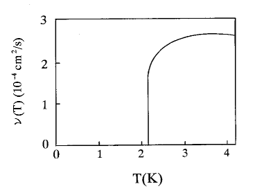
Figure 1: The temperature dependence of the kinematic shear viscosity $\nu(T)$ of liquid helium 4 obtained in Ref.bar .

London stressed that the total disappearance of shear viscosity is attributed to $rot\mbox{\boldmath$v$}=0$ over the whole volume of a liquid lod . The partial disappearance of shear viscosity at $T_{\lambda}<T<3.7K$ in Fig.1 suggests the emergence of regions in which $rot\mbox{\boldmath$v$}=0$ is locally realized. Compared to an ordinary liquid, liquid helium 4 above $T_{\lambda}$ has a $10^{-3}$ times smaller coefficient of shear viscosity. Although in the normal phase, it is already an anomalous liquid under the strong influence of Bose statistics. Hence, it seems natural to assume the existence of large but not yet macroscopic coherent wave functions koh . If there exist such intermediate-sized wave functions above $T_{\lambda}$, they must affect the macroscopic flow.

In conventional theories, we normally do not think of the large but not yet macroscopic wave function. This is because we use the infinite volume limit ($V\rightarrow\infty$) in order to make a clear definition of the order parameter in the phase transition. In the $V\rightarrow\infty$ limit, “large but not yet macroscopic” is equivalent to “microscopic”, and therefore the intermediate-sized wave function disappears from the beginning. For the system in which the distinction between “microscopic” and “macroscopic” is clear, the $V\rightarrow\infty$ limit is a realistic one. For the Bose system at low temperature, however, the Bose statistical coherence develops to a macroscopic or an intermediate size, and the container and the coherent region of a liquid are comparable in size. The $V\rightarrow\infty$ limit is therefore a questionable assumption for considering the mechanical properties of the Bose system just above $T_{\lambda}$. (For the thermodynamical properties, we encounter no difficulty in the $V\rightarrow\infty$ limit.)

The shear viscosity of liquid helium 4 has been subjected to considerable experimental and theoretical studies. These studies are mainly focused on the famous paradox at $T<T_{\lambda}$ that superfluid helium 4 behaves as a viscous or non-viscous fluid, depending on the experimental methods. For $\nu(T)$ at $T_{\lambda}<T<3.7K$, it is often said that it resembles $\nu(T)$ of a gas rather than a liquid in its magnitude and in its temperature dependence. But this explanation is somewhat misleading. In liquid helium 4, many features associated to Bose statistics have been masked by the strongly interacting nature of the liquid. Well below the lambda point $T_{\lambda}$, various excitations of liquid helium 4 are strictly suppressed except for phonons and rotons. Hence, although the excitation in a liquid, these phonons and rotons are normally regarded as a weakly interacting dilute Bose gas kha . For $\nu(T)$ above $T_{\lambda}$, however, the dilute-gas picture has no grounds, because the macroscopic condensate, which is the basis for the above picture, has not yet developed. To explain $\nu(T)$ above $T_{\lambda}$, we must deal with the dissipation mechanism of a liquid and the influence of Bose statistics on it.

At present, for the accuracy of data, the early measurements of $\eta(T)$ using the capillary have been superseded by new measurements using more accurate techniques such as the vibrating wire goo wel bru . Above the $\lambda$ point, the latter method gives not only quantitatively similar, but more precise data of $\eta(T)$. Applying the statistical analysis to these accumulated data, a precise temperature dependence of $\eta(T)$ and $\nu(T)$ above $T_{\lambda}$ was obtained bar . A theory worth comparing with these precise data is desired.

This paper gives a model of the onset of superfluid flow in the capillary. Instead of assuming the macroscopic condensate from the beginning, we begin with the repulsive Bose system with no off-diagonal-long-range order (ODLO), and show that, with decreasing temperature above $T_{\lambda}$, the coherent many-body wave function gradually grows. In Ref.koh , we showed that this growth reflects in the rotational properties such as the moment of inertia above $T_{\lambda}$. In contrast with the rotation, however, the capillary flow of a classical liquid is a phenomenon that is accompanied by thermal dissipation. The frictionless capillary flow at $T<T_{\lambda}$ is superfluidity which occurs in the strongly dissipative system when it is at $T>T_{\lambda}$. Hence, to consider this phenomenon, we must devise a different formalism. To take the nature of the liquid into consideration, we will go back to fluid mechanics in the normal phase, and begin with the solution of the Stokes equation for the capillary flow (Poiseuille formula). The capillary flow is embedded into a general picture that is applicable both to dissipative and to non-dissipative flows using the generalized susceptibility. Applying the Kramers-Kronig relation to the generalized susceptibility, we relate the capillary flow to its non-dissipative counterpart, rotating helium 4 in a bucket, and derive the decrease of $\nu(T)$ from the growth of the coherent wave function. When this result is combined with that in Ref.koh , we come to understand the onset of two types of superfluidity in the shear viscosity and in the moment of inertia from a common origin.

This paper is organized as follows. Section.2 examines the capillary flow in terms of the generalized susceptibility. Using this method, Sec.3A gives a formula for the shear viscosity in the vicinity of $T_{\lambda}$, and Sec.3B examines the role of Bose statistics and the repulsive interaction in the suppression of the shear viscosity. Section.4 develops a microscopic model of the onset of the superfluid flow. By generalizing the formalism in Ref.koh to the time-dependent case, we derive the decrease of $\eta$ just above $T_{\lambda}$ from the growth of the coherent wave function, and discuss the stability of superfluid flow through a capillary. To describe the system just above $T_{\lambda}$, the mechanical superfluid density $\hat{\rho}_{s}(T)$, which is defined without using $V\rightarrow\infty$, is more useful than the conventional superfluid density $\rho_{s}(T)$. In Sec.5, using $\nu(T)$ of Fig.1, we estimate the ratio $\hat{\rho_{s}}(T)/\rho$, and compare this $\hat{\rho_{s}}(T)/\rho$ with another $\hat{\rho_{s}}(T)/\rho$ obtained by the rotation experiment hes . Section.6 discusses some related problems.

II Capillary flow

In an ordinary liquid flowing along x-direction, the shear viscosity causes the shear stress $F_{xy}$ between two adjacent layers at different velocities (see Fig.2)

$$F_{xy}=\eta\frac{\partial v_{x}}{\partial y}.$$ (1)

In the linear-response theory, $\eta$ of a stationary flow is given by the following two-time correlation function of a tensor $J_{xy}(t)=-\sum_{i}(p_{i,x}p_{i,y}/m)$

$$\eta=\frac{1}{Vk_{B}T}\int_{0}^{\infty}dt<J_{xy}(0)J_{xy}(t)>.$$ (2)

In principle, $\eta$ of a liquid, and therefore the effect of Bose statistics on $\eta$ is obtained by calculating an infinite series of the perturbation expansion of Eq.(2) with respect to the particle interaction. However, it seems to be a hopeless attempt, because the dissipation in a liquid is a complicated phenomenon that allows no simple approximation han .

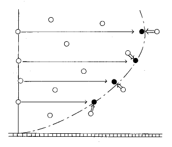
Figure 2: A flow through a capillary.

Fluid mechanics is a simple phenomenological theory of non-equilibrium behaviors for situations in which physical quantities vary slowly in space and time. In this paper, we will develop an intermediate theory between the microscopic and phenomenological one kad , and derive some information on the shear viscosity from the correspondence between these two different levels of description. In an ordinary flow through a capillary with a circular cross-section (a radius $d$ and a length $L$), the Stokes equation has a solution of the velocity distribution $v_{z}(r)$ under the pressure difference $\Delta P$ such as

$$v_{z}(r)=\frac{d^{2}-r^{2}}{4\eta}\frac{\Delta P}{L},$$ (3)

where $r$ is a radius in the cylindrical coordinates (Poiseuille flow lan . Fig.2). Without loss of generality, we may focus on a flow velocity on the axis of rotational symmetry (z-axis). We define a mass-flow density $\mbox{\boldmath$j$}=\rho\mbox{\boldmath$v$}(r=0)$, and rewrite Eq.(3) as

$$\mbox{\boldmath$j$}=-\sigma d^{2}\frac{\Delta\mbox{\boldmath$P$}}{L},\qquad\sigma=\frac{\rho}{4\eta}.$$ (4)

We call $\sigma$ the conductivity of a viscous liquid flow through a capillary ($\mbox{\boldmath$P$}=P\mbox{\boldmath$e$}_{z}$) cur . From a microscopic view point, it is a long-standing problem to derive the absolute value of $\eta$ using Eq.(2) jeo . In this paper, however, instead of Eq.(2), we will regard Poiseuille’s formula Eq.(4) as a starting point. We regard Eq.(4) as a phenomenological linear-response relation, and compare it to the microscopic formula for the mass-flow density $j$ like Eq.(28). By this comparison, we will extract only the change of $\eta$ near $T_{\lambda}$ from the total $\eta$ in Sec.3, and derive this change from a microscopic model in Sec.4.

In a flow through a capillary set up vertically, the level of a liquid in the reservoir varies with time $t$ as $h(t)=h(0)e^{-\alpha t}$ (see Appendix.A). Hence, $\Delta P(t)$ in Eq.(4) decreases as $\Delta P(t)=\Delta P(0)e^{-\alpha t}$ as well. With the aid of

$$e^{-\alpha t}=\frac{1}{\pi}\int_{0}^{\infty}\frac{1}{\sqrt{\omega^{2}+\alpha^{2}}}e^{i(\omega t-\phi)}d\omega,$$ (5)

($\tan\phi=\omega/\alpha$), $\Delta\mbox{\boldmath$P$}(t)$ is decomposed into the frequency components $\Delta\mbox{\boldmath$P$}(\omega)$ within a range of $[0,\omega_{e}]$ where $\omega_{e}$ is a frequency width. Let us generalize Eq.(4) to the case of $\mbox{\boldmath$j$}(\omega)e^{i\omega t}$ under the oscillatory pressure $\mbox{\boldmath$P$}(\omega)e^{i\omega t}$ as follows

$$\mbox{\boldmath$j$}(\omega)=-\sigma(\omega)d^{2}\frac{\Delta\mbox{\boldmath$P$}(\omega)}{L}.$$ (6)

The conductivity spectrum $\sigma(\omega)$ must satisfy the following sum rule sum

$$\frac{1}{\pi}\int_{0}^{\infty}\sigma(\omega)d\omega=f(d),$$ (7)

where $f(d)$ is a conserved quantity. (The Stokes equation gives an expression of $\sigma(\omega)$ and $f(d)$ of the classical liquid. See Appendix.B.) In Eq.(4), we must incorporate the effect of time variation of $\Delta\mbox{\boldmath$P$}(t)$ into $j$ and $\sigma$, and we define the frequency-averaged $\sigma$ as $\sigma=\omega_{e}^{-1}\int_{0}^{\omega_{e}}\sigma(\omega)d\omega$ using $\sigma(\omega)$ in Eq.(6) .

The change of the starting point from Eq.(2) to Eq.(4) permits us to relate different types of superfluidity: (a) the frictionless capillary flow, and (b) the nonclassical flow in a rotating bucket. The phenomenological equation (6) is appropriate to be generalized so as to include different types of superfluidity. Such a method originated in studies of electron superconductivity fer . Between the electrical conduction and the Meissner effect in superconductivity, we find a relationship parallel to the relationship between the capillary flow and the rotational flow in superfluidity,

The generalization of Eq.(6) is as follows. The conductivity spectrum $\sigma(\omega)$, which describes the dissipative response of a liquid, corresponds to an imaginary part of the generalized susceptibility $\chi(\omega)$ that describes both dissipative and non-dissipative responses of a liquid. We will generalize Eq.(6) so as to include not only a response in phase with $\Delta\mbox{\boldmath$P$}(\omega)$ but a response out of phase. Hence, $\sigma(\omega)$ in Eq.(6) becomes a complex number $\sigma_{1}+i\sigma_{2}$ as follows

$$\mbox{\boldmath$j$}(\omega)=-\left[\sigma_{1}(\omega)+i\sigma_{2}(\omega)\right]d^{2}\frac{\Delta\mbox{\boldmath$P$}(\omega)}{L},$$ (8)

where $\sigma(\omega)$ in Eq.(6) is replaced by $\sigma_{1}(\omega)$. The application of the pressure gradient can be fitted into the general picture as follows. As an external field, we assume a fictitious velocity $\mbox{\boldmath$v$}(t)$ that satisfies the equation of motion vec

$$\rho\frac{d\mbox{\boldmath$v$}(t)}{dt}=-\frac{\Delta\mbox{\boldmath$P$}(t)}{L},$$ (9)

and replace $\Delta\mbox{\boldmath$P$}(\omega)/L$ in Eq.(8) with $-i\rho\omega\mbox{\boldmath$v$}(\omega)$ using Eq.(9). As a result, the real and imaginary part of $\sigma(\omega)$ are interchanged vel ,

$$\mbox{\boldmath$j$}(\omega)=\rho\left[-\omega\sigma_{2}(\omega)+i\omega\sigma_{1}(\omega)\right]d^{2}\mbox{\boldmath$v$}(\omega).$$ (10)

Equation (10) is our desired formula, the coefficient of which consists not only of an imaginary part $i\omega\sigma_{1}(\omega)$ for the dissipative flow, but of a real part $-\omega\sigma_{2}(\omega)$ for the non-dissipative one, thus forming the generalized susceptibility. According to the choice of $\mbox{\boldmath$v$}(\omega)$, Eq.(10) expresses different types of flow, but the generalized susceptibility has a general structure independent of the flow type. This means that by relating $\sigma_{1}(\omega)$ to $\sigma_{2}(\omega)$, we can derive $\sigma_{1}(\omega)$ of a capillary flow from $\sigma_{2}(\omega)$ of a non-dissipative flow. Causality requires that fluid particles begins to flow only after the pressure is applied. We can use the following Kramers-Kronig relation for $-\omega\sigma_{2}(\omega)$ and $\omega\sigma_{1}(\omega)$ in Eq.(10)

$$\sigma_{1}(\omega^{\prime})=\frac{2}{\pi}\int_{0}^{\infty}d\omega\frac{\omega\sigma_{2}(\omega)}{\omega^{2}-\omega^{\prime 2}},$$ (11)

$$\sigma_{2}(\omega^{\prime})=-\frac{2\omega^{\prime}}{\pi}\int_{0}^{\infty}d\omega\frac{\sigma_{1}(\omega)}{\omega^{2}-\omega^{\prime 2}}.$$ (12)

If one determines $\sigma_{2}(\omega)$ in the non-dissipative flow, one can obtain $\sigma_{1}(\omega)$ using Eq.(11), hence $\sigma(\omega)$ in Eq.(6).

As a non-dissipative flow, we will consider the flow in a rotating bucket. In a rotating bucket, a liquid makes the rigid-body rotation owing to its viscosity. The rotational velocity, which is used as $\mbox{\boldmath$v$}(\omega)$ in Eq.(10), is a product of the angular velocity $\Omega$ and the radius $r$ such as $\mbox{\boldmath$v$}_{d}(\mbox{\boldmath$r$})\equiv\mbox{\boldmath$\Omega$}\times\mbox{\boldmath$r$}$. For this $\mbox{\boldmath$v$}_{d}(\mbox{\boldmath$r$})$, the dissipation function lan

$$\Phi(\mbox{\boldmath$r$})=2\eta\left(e_{ij}-\frac{1}{3}e_{kk}\delta_{ij}\right)^{2}$$ (13)

is zero at every $r$, where $2e_{ij}=\partial v_{i}/\partial x_{j}+\partial v_{j}/\partial x_{i}$. This means that, except at the boundary to the wall, there is no frictional force within a liquid even in the normal phase, and the rigid-body rotation is therefore a non-dissipative flow. (On the other hand, for the Poiseuille flow Eq.(3), Eq.(13) is not zero at every $r$ except for $r=0$. Fluid particles in the capillary flow experience thermal dissipation not only at the boundary, but within the flow.)

The flow in a rotating bucket is formulated using the generalized susceptibility of the system $\chi(\mbox{\boldmath$r$},\omega)$ noz (see Appendix.C), which is decomposed to the longitudinal and transverse part ($\mu,\nu=x,y,z$)

$$\chi_{\mu\nu}(q,\omega)=\frac{q_{\mu}q_{\nu}}{q^{2}}\chi^{L}(q,\omega)+\left(\delta_{\mu\nu}-\frac{q_{\mu}q_{\nu}}{q^{2}}\right)\chi^{T}(q,\omega).$$ (14)

In the flow in a rotating bucket, the influence of the bucket propagates along the radial direction from the wall to the center, which is perpendicular to the particle motion driven by rotation (Fig.2 of Ref.koh ). Hence, the flow in a rotating bucket is a transverse response of the system described by the transverse susceptibility $\chi^{T}(q,\omega)$. In the right-hand side of Eq.(10), the real part of the susceptibility $-\rho\omega\sigma_{2}(\omega)d^{2}$ is expressed as

$$-\rho d^{2}\omega\sigma_{2}(\omega)=\lim_{q\rightarrow 0}\chi^{T}(q,\omega).$$ (15)

Now, we can express the conductivity of the capillary flow in terms of the susceptibility of the system. Using Eq.(15) in the right-hand side of Eq.(11), we obtain $\sigma_{1}(\omega)$ for the capillary flow

$$\rho d^{2}\sigma_{1}(\omega^{\prime})=-\frac{2}{\pi}\int_{0}^{\infty}d\omega\frac{\lim_{q\rightarrow 0}\chi^{T}(q,\omega)}{\omega^{2}-\omega^{\prime 2}}.$$ (16)

Quantum mechanics states that, in the decay from an excited state with an energy level $E$ to a ground state with $E_{0}$, the higher excitation energy $E$ causes the shorter relaxation time $\tau$, $\hbar/\tau\simeq|E-E_{0}|$. In Eq.(16), the left-hand side includes the relaxation time $\tau$ in $\sigma_{1}=\rho/(4\eta)=\rho/(4G\tau)$, whereas the right-hand side includes the excitation spectrum in $\chi^{T}(q,\omega)$. (We used Maxwell’s relation $\eta=G\tau$ max . See Appendix.D.) In this sense, Eq.(16) is a many-body theoretical expression of $\hbar/\tau\simeq|E-E_{0}|$.

III Shear viscosity of a superfluid

III.1 Phenomenological argument

In the superfluid phase, even when the pressure difference vanishes ($\Delta P=0$) in Eq.(4), one observes a stable flow, hence $\eta=0$. The essence of superfluidity is that the normal-fluid and superfluid part flows without any transfer of momentum from one to the other. Characteristic to the frictionless flow in Eq.(6) is that in addition to the normal fluid part $\sigma_{n}(\omega)$, the conductivity spectrum $\sigma(\omega)$ has a sharp peak at $\omega=0$

$$\mbox{\boldmath$j$}(\omega)=-\left[\sigma_{n}(\omega)+A\delta(\omega)\right]d^{2}\frac{\Delta\mbox{\boldmath$P$}(\omega)}{L},$$ (17)

where $A\delta(\omega)$ is a simplified expression of the sharp peak at $\omega=0$ with an area $A$ fer . Figure 3 schematically illustrates such a change of $\sigma(\omega)$ when the system passes $T_{\lambda}$. The separation of the sharp peak from $\sigma_{n}(\omega)$ guarantees the absence of the momentum transfer (except for $\sigma_{n}(\omega)$ near $\omega=0$ due to the acoustic phonon). When $\sigma(\omega)$ has a form of $\sigma_{n}(\omega)+A\delta(\omega)$, it affects the conductivity $\sigma=\omega_{e}^{-1}\int_{0}^{\omega_{e}}\sigma(\omega)d\omega$, and $\eta$ in Eq.(4) is given by

$$\eta(T)=\frac{1}{4}\frac{\rho}{\displaystyle{\omega_{e}^{-1}\left(\int_{0}^{\omega_{e}}\sigma_{n}(\omega)d\omega+A\right)}}.$$ (18)

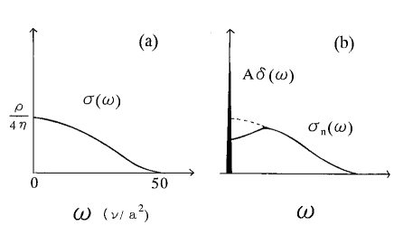
Figure 3: The change of the conductivity spectrum $\sigma(\omega)$ from (a) in a classical fluid to (b) in a superfluid. $\sigma(\omega)$ is given by Eq.(B6) in Appendix.B.

Equation (18) is explained by the following argument on the susceptibility.

(1) In the classical fluid, $\chi^{L}(q,\omega)=\chi^{T}(q,\omega)$ is satisfied at small $q$, and one can replace $\chi^{T}(q,\omega)$ in Eq.(16) by $\chi^{L}(q,\omega)$ for a small $q$ def . Hence, in the classical fluid the conductivity $\sigma_{1n}(\omega)$ of the capillary flow is given by

$$\rho d^{2}\sigma_{1n}(\omega^{\prime})=-\frac{2}{\pi}\int_{0}^{\infty}d\omega\frac{\lim_{q\rightarrow 0}\chi^{L}(q,\omega)}{\omega^{2}-\omega^{\prime 2}}.$$ (19)

In the superfluid phase, however, under the strong influence of Bose statistics, the condition of $\chi^{L}(q,\omega)=\chi^{T}(q,\omega)$ at $q\rightarrow 0$ is violated (see Sec.3B and 4). Hence, one cannot replace $\chi^{T}(q,\omega)$ by $\chi^{L}(q,\omega)$ in Eq.(16), and must express Eq.(16) using Eq.(19) as follows

$$\sigma_{1}(\omega^{\prime})=\sigma_{1n}(\omega^{\prime})+\frac{2}{\rho\pi d^{2}}\int_{0}^{\infty}d\omega\frac{\lim_{q\rightarrow 0}[\chi^{L}(q,\omega)-\chi^{T}(q,\omega)]}{\omega^{2}-\omega^{\prime 2}},$$ (20)

in which $\lim_{q\rightarrow 0}[\chi^{L}(q,\omega)-\chi^{T}(q,\omega)]$ corresponds to a superfluid component. For the later use, we define a term proportional to $q_{\mu}q_{\nu}$ in $\chi_{\mu\nu}$ by $\hat{\chi}_{\mu\nu}$ as a quantity representing the balance between the longitudinal and transverse response as follows

$$\chi_{\mu\nu}(q,\omega) = \delta_{\mu\nu}\chi^{T}(q,\omega)+q_{\mu}q_{\nu}\left(\frac{\chi^{L}(q,\omega)-\chi^{T}(q,\omega)}{q^{2}}\right)$$ (21)

$$\equiv \delta_{\mu\nu}\chi^{T}(q,\omega)+\hat{\chi}_{\mu\nu}(q,\omega).$$

(2) The stability of a superfluid is measured by the value of $\chi^{L}(q,\omega)-\chi^{T}(q,\omega)$ at the finite $\omega$. In general, the superfluid flow is not perfectly stable with respect to oscillating external perturbations. Above a certain frequency, $\chi^{L}(q,\omega)-\chi^{T}(q,\omega)$ vanishes, and the system behaves as a classical fluid. (In Sec.4, we will show this using a concrete model.)

(3) The shear viscosity near $T_{\lambda}$ is mainly determined by the value of $\lim_{q\rightarrow 0}[\chi^{L}(q,\omega)-\chi^{T}(q,\omega)]$ in the vicinity of $\omega=0$. In the right-hand side of Eq.(20), the finiteness of $\chi^{L}(q,\omega)-\chi^{T}(q,\omega)$ at $\omega\simeq 0$ leads to a sharp peak at $\omega^{\prime}=0$, because of

$$\int_{0}^{\infty}\frac{d\omega}{\omega^{2}-\omega^{\prime 2}}=\delta(\omega^{\prime}).$$ (22)

Hence, in the superfluid phase, $\sigma_{1}(\omega^{\prime})$ shows a peculiar peak at $\omega^{\prime}=0$ like that in Fig.3.(b). (Since this change obeys the sum rule Eq.(7), the area $A$ of the sharp peak is equal to the area enclosed by a dotted and a solid curve in Fig.3(b).)

(4) From now, we approximate $\chi^{L}(q,\omega)-\chi^{T}(q,\omega)$ by its value at $\omega=0$ in Eq.(20), and $\sigma_{1}(\omega)$ has a form such as

$$\sigma_{1}(\omega)=\sigma_{1n}(\omega)+\frac{2}{\rho\pi d^{2}}\lim_{q\rightarrow 0}[\chi^{L}(q,0)-\chi^{T}(q,0)]\delta(\omega).$$ (23)

As the temperature decreases from $T_{\lambda}$, the area of the sharp peak increases. Using Eq.(23) in Eq.(18), one obtains the coefficient of shear viscosity

$$\eta(T)=\left(\frac{\rho}{4}\right)\frac{1}{\sigma_{1n}+\displaystyle{\frac{2}{\rho\pi d^{2}\omega_{e}}\lim_{q\rightarrow 0}[\chi^{L}(q,0)-\chi^{T}(q,0)]}}.$$ (24)

Here, we define the mechanical superfluid density $\hat{\rho_{s}}(T)\equiv\lim_{q\rightarrow 0}[\chi^{L}(q,0)-\chi^{T}(q,0)]$ ($=\lim_{q\rightarrow 0}[\hat{\chi}_{\mu\nu}(q,0)q^{2}/(q_{\mu}q_{\nu})]$), which does not always agree with the conventional thermodynamical superfluid density $\rho_{s}(T)$. (By “thermodynamical”, we imply the quantity that remains finite in the $V\rightarrow\infty$ limit.)

Since the total density $\rho$ in Eq.(24) slightly increases with decreasing temperature from $4.2K$ to $T_{\lambda}$ ker , the kinematic shear viscosity $\nu(T)=\eta(T)/\rho(T)$ is more appropriate than $\eta(T)$ to describe the change of the system around $T_{\lambda}$. We obtain a formula of $\nu(T)=\eta(T)/\rho(T)$ as follows

$$\nu(T)=\frac{\nu_{n}}{1+\displaystyle{\frac{8}{\pi d^{2}\omega_{e}}\frac{\hat{\rho_{s}}(T)}{\rho}}\nu_{n}},$$ (25)

where $\nu_{n}$ is the kinematic shear viscosity of a classical fluid, and satisfies $\sigma_{1n}=\rho/(4\eta_{n})=1/(4\nu_{n})$ in Eq.(24). In general, $\nu_{n}(T)$ of the classical liquid has the property of increasing monotonically with decreasing temperature she . In Fig.1, $\nu(T)$ above $3.7K$ seems to show this property, but its gradual fall below $3.7K$ cannot be explained by the classical liquid picture, thereby suggesting $\hat{\rho_{s}}(T)\neq 0$ in Eq.(25) at $T_{\lambda}\leq T\leq 3.7K$.

In the free Bose system, using $j_{\mu}(q,\tau)$ in Eq.(C2), $\hat{\chi}_{\mu\nu}(q,\omega)$ in Eq.(21) has a form of

$$\hat{\chi}^{(1)}_{\mu\nu}(q,\omega)=-\frac{q_{\mu}q_{\nu}}{4}\frac{1}{V}\sum_{p}\frac{f(\epsilon(p))-f(\epsilon(p+q))}{\omega+\epsilon(p)-\epsilon(p+q)},$$ (26)

where $f(\epsilon(p))=\exp(\beta[\epsilon(q)+\Sigma-\mu])-1)^{-1}$ is the Bose distribution, $\Sigma$ is a self energy of a boson (we ignore $\omega$ and $p$ dependence of $\Sigma$ by assuming it small), and $\mu$ is a chemical potential. At $T<T_{\lambda}$, $f(\epsilon(p))$ is a macroscopic number for $p=0$, and nearly zero for $p\neq 0$. Hence, in the sum over $p$, only two terms corresponding to $p=0$ and $p=-q$ remain. This means that $\hat{\chi}^{(1)}_{\mu\nu}(q,0)$ has a form of $\hat{\rho_{s}}(T)q_{\mu}q_{\nu}/q^{2}$. Practically, a nonzero $\hat{\rho_{s}}(T)$ and a small $\omega_{e}$ vanishes $\nu(T)$ at $T<T_{\lambda}$ in Eq.(25). When bosons form no condensate, however, the sum over $p$ in Eq.(26) is carried out by replacing it with an integral, and $q^{-2}$ dependence of $\hat{\chi}^{(1)}_{\mu\nu}(q,0)$ disappears, hence $\hat{\rho_{s}}(T)=0$ and $\nu(T)$ remains finite. This means that, without the interaction between particles, the macroscopic Bose-Einstein condensation (BEC) is the necessary condition for the decrease of $\nu(T)$. To explain the gradual fall of $\nu(T)$ just above $T_{\lambda}$, we must obtain $\chi^{L}(q,\omega)-\chi^{T}(q,\omega)$ under the particle interaction.

III.2 The effect of Bose statistics and repulsive interaction

One can physically explain the fall of the shear viscosity in Eq.(25) in terms of Bose statistics. When a liquid flows through a capillary, it moves in the same direction but with a speed that varies in a perpendicular direction. For the classical liquid, Maxwell obtained a simple formula $\eta=G\tau_{st}$ (Maxwell’s relation. See Appendix.D) max , where $G$ is the modulus of rigidity, and $\tau_{st}$ is a characteristic time of structural relaxations that occur under the sheer stress in the flow. (The reader must not confuse this $\tau_{st}$ with $\tau_{th}$ of thermal fluctuations.) This relation is useful for the interpretation of liquid helium 4 as well. In the vicinity of $T_{\lambda}$ in liquid helium 4, no structural transition is observed in coordinate space. Hence, $G$ may be a constant at the first approximation, and therefore the fall of the shear viscosity is attributed mainly to the decrease of $\tau_{st}$. In view of $\hbar/\tau_{st}\simeq|E-E_{0}|$, the decrease of $\tau_{st}$ suggests the increase of the excitation energy $E$, and it is natural to attribute it to Bose statistics. The relationship between the excitation energy and Bose statistics dates back to Feynman’s argument on the scarcity of the low-energy excitation in liquid helium 4 fey1 , in which he explained how Bose statistics affects the many-body wave function in configuration space. To the shear viscosity, we will apply his explanation.

Consider a flow in Fig.2, in which white circles represent an initial distribution of fluid particles. The long thin arrows represent the displacement from white circles on a solid straight line to black circles on a one-point-dotted-line curve. (The influence of adjacent layers in a viscous flow propagates along a direction perpendicular to the particle motion. Hence, the excitation associated with the shear viscosity is a transverse one.) Let us assume that a liquid in Fig.2 is in the BEC phase, and the many-body wave function has permutation symmetry everywhere in a capillary. At first sight, these displacements by long arrows seem to be a large-scale configuration change, but they are reproduced by a set of slight displacements by short thick arrows from the neighboring white circles in the initial distribution. In general, the transverse modulation, such as the displacement by shear viscosity, does not change the particle density in the large scale, and therefore, to any given particle after displacement, it is always possible to find such a neighboring particle in the initial distribution. In Bose statistics, owing to permutation symmetry, one cannot distinguish between two types of particles after displacement, one moved from the neighboring position by the short arrow, and the other moved from distant initial positions by the long arrow. Even if the displacement made by the long arrows is a large displacement in classical statistics, it is only a slight displacement by the short arrows in Bose statistics . (In contrast, the longitudinal modulation results in the large-scale inhomogeneity in the particle density, and therefore it is not always possible to find such neighboring initial positions.)

Let us imagine this situation in 3N-dimensional configuration space. The excited state made of slight displacements, which is characteristic of Bose statistics, lies in a small distance from the ground state in configuration space. On the other hand, the wave function of the excited state is orthogonal to that of the ground state in the integral over configurations. Since the amplitude of the ground-state wave function is uniform in principle, the amplitude of the excited-state wave function must spatially oscillate around zero. Accordingly, the wave function of the excited state must oscillate around zero within a small distance in configuration space. The kinetic energy of the system is determined by the 3N-dimensional gradient of the many-body wave function in configuration space, and therefore this steep rise and fall of the amplitude raises the excitation energy of this wave function. The relaxation from such an excited state is a rapid process with a small $\tau_{st}$. This mechanism explains why Bose statistics leads to the small coefficient of shear viscosity $\eta=G\tau_{st}$.

When the system is at high temperature, the coherent wave function has a microscopic size. If a long arrow in Fig.2 takes a particle out of the coherent wave function, one cannot regard the particle after displacement as an equivalent of the initial one. The mechanism below $T_{\lambda}$ does not work for the large displacement extending over two different wave functions. Hence, the relaxation time $\tau_{st}$ changes to an ordinary long $\tau_{st}$, which is characteristic of the classical liquid ber .

When the system is just above $T_{\lambda}$, the size of the coherent wave function is not yet macroscopic, but it develops to an intermediate size. In the repulsive system with high density, the long-distance displacements of particles takes much energy, and therefore particles in the low-energy excitation are likely to stay within the same wave function. The excitation energy is not so high as that of the long-distance displacements, but owing to Bose statistics, it is not so low as that of the classical liquid. Fast relaxations within these wave functions is the reason for the decrease of $\eta$ in the macroscopic capillary flow. (In contrast, the ideal Bose system is too simple for such a situation to be realized, in which the macroscopic condensate at $T<T_{\lambda}$ is a necessary condition for the decrease of $\eta$ as in Eq.(26).)

IV A model of the onset of superfluid flow

Let us develop a microscopic model of the onset of superfluid flow. In deriving the shear viscosity $\eta$, Eq.(4) has the following advantage over Eq.(2). In the weak-coupling system (a gas, and a simple liquid like liquid helium 4), the particle interaction $U$ normally enhances the relaxation of individual particles to local equilibrium positions under a given external force, thereby leading to small $\tau_{st}$ and $\eta=G\tau_{st}$ stro . If we try to formulate this tendency using Eq.(2), that is, to derive a decrease of $\eta$ from an increase of $U$ in Eq.(2), there must be delicate cancellation of higher-order terms in the perturbation expansion of $<J_{xy}(0)J_{xy}(t)>$. On the contrary, if we regard Eq.(4), in which $\eta$ appears in the denominator of $\sigma$, as a linear-response relation, we apply the Kubo formula not to $\eta$ but to the reciprocal $1/\eta$. In the perturbation expansion of $1/\eta$ with respect to $U$, an increase of $U$ generally leads to an increase of $1/\eta$ and thereby a decrease of $\eta$ . Hence, one need not expect the cancellation. In this respect, when we use Eq.(4) as a starting point, the influence of $U$ on $\eta$ is naturally built into the formalism from the beginning.

IV.1 The onset of nonclassical behavior

For liquid helium 4, we use the following hamiltonian with the repulsive interaction $U$

$$H=\sum_{p}\epsilon(p)\Phi_{p}^{\dagger}\Phi_{p}+U\sum_{p,p^{\prime}}\sum_{q}\Phi_{p-q}^{\dagger}\Phi_{p^{\prime}+q}^{\dagger}\Phi_{p^{\prime}}\Phi_{p},\qquad(U>0),$$ (27)

where $\Phi_{p}$ denotes an annihilation operator of a spinless boson. Beginning with the repulsive Bose system with no ODLO, we make a perturbation expansion. Under the particle interaction $\hat{H_{I}}(\tau)$, $\chi_{\mu\nu}(q,\omega)$ is derived from

$$<G|T_{\tau}j_{\mu}(x,\tau)j_{\nu}(0,0)|G>=\frac{\displaystyle{<0|T_{\tau}\hat{j}_{\mu}(x,\tau)\hat{j}_{\nu}(0,0)exp\left[-\int_{0}^{\beta}d\tau\hat{H}_{I}(\tau)\right]|0>}}{\displaystyle{<0|exp\left[-\int_{0}^{\beta}d\tau\hat{H}_{I}(\tau)\right]|0>}},$$ (28)

where $\beta=1/(k_{B}T),\tau=it$, and $\hat{j}_{\mu}(x,\tau)$ is an interaction representation of Eq.(C2).

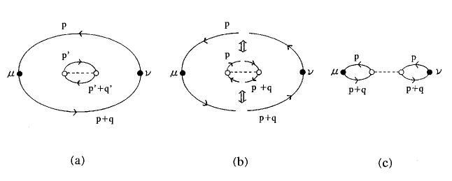
Figure 4: When $p=p^{\prime}$ and $p+q=p^{\prime}+q^{\prime}$ in (a), an exchange of particles in (b) between $j_{\mu}j_{\nu}$ (a large bubble) and a bubble excitation by $\hat{H}_{I}$ (a small one) yields (c).

The current-current response tensor $\hat{j}_{\mu}(x,\tau)\hat{j}_{\nu}(0,0)$ (a large bubble with $\mu$ and $\nu$ in Fig.4(a)) is in the medium in which particles experience the repulsive interaction: Owing to $exp(-\smallint\hat{H}_{I}(\tau)d\tau)$ in Eq.(28), scattering of particles frequently occurs in the medium, an example of which is illustrated by an inner small bubble with a dotted line $U$ in Fig.4(a). As the system approaches $T_{\lambda}$, $\hat{j}_{\mu}(x,\tau)\hat{j}_{\nu}(0,0)$ and $\hat{H}_{I}(\tau)$ in Eq.(28) get to obey Bose statistics strictly, that is, the particles in the large and small bubbles in Fig.4(a) form a coherent wave function as a whole com : When one of the two particles in the large bubble and in the small bubble have the same momentum ($p=p^{\prime}$), and when the other particles in both bubbles have another same momentum ($p+q=p^{\prime}+q^{\prime}$), owing to Bose statistics, a graph made by exchanging these particles must be included in the expansion of Eq.(28). The cutting and reconnection of these lines between the large and small bubbles in Fig.4(b) yields Fig.4(c), in which two bubbles with the same momenta are linked by the repulsive interaction. With decreasing temperature, the coherent wave function grows, and such an exchange of particles occurs many times. Furthermore, with deceasing temperature, particles with the zero momentum get to play a more dominant role than others. In Fig.4, this means that taking only processes including zero-momentum particles becomes a good approximation: In $j_{\mu}j_{\nu}$ of Eq.(26), a bubble with $p=0$ corresponds to an excitation from the rest particle, and a bubble with $p=-q$ corresponds to a decay into the rest one. Taking only such processes and continuing these exchanges, one obtains

$$\hat{\chi}_{\mu\nu}(q,i\omega)=\frac{q_{\mu}q_{\nu}}{4}\frac{1}{V}\left[\frac{F_{\beta}(q,i\omega)}{1-UF_{\beta}(q,i\omega)}+\frac{F_{\beta}(q,-i\omega)}{1-UF_{\beta}(q,-i\omega)}\right],$$ (29)

where the first and second term in the right-hand side corresponds to the $p=0$ and $p=-q$ term in Eq.(26), respectively, and

$$F_{\beta}(q,i\omega)=\frac{(\exp(\beta[\Sigma-\mu])-1)^{-1}-(\exp(\beta[\epsilon(q)+\Sigma-\mu])-1)^{-1}}{-i\omega+\epsilon(q)}.$$ (30)

Let us focus on the low-energy excitations. For a small $\omega$, the first term in the bracket of the right-hand side of Eq.(29) is expanded with respect to $\omega$ as

$$\frac{F_{\beta}(q,i\omega)}{1-UF_{\beta}(q,i\omega)} = \frac{f(\epsilon(0))-f(\epsilon(q))}{\epsilon(q)-U[f(\epsilon(0))-f(\epsilon(q))]}$$

$$\times \left[1+\frac{i\omega}{\epsilon(q)-U[f(\epsilon(0))-f(\epsilon(q))]}+\frac{(i\omega)^{2}}{2(\epsilon(q)-U[f(\epsilon(0))-f(\epsilon(q)])^{2}}\cdots\right].$$

Hence, Eq.(29) is expanded as

$$\hat{\chi}_{\mu\nu}(q,\omega)=\frac{q_{\mu}q_{\nu}}{4}\frac{1}{V}\frac{2F_{\beta}(q,0)}{1-UF_{\beta}(q,0)}\left[1-\left(\frac{\omega}{\epsilon(q)(1-UF_{\beta}(q,0))}\right)^{2}+\cdots\right].$$ (32)

Since the macroscopic flow is of our interest, let us focus on $\hat{\chi}_{\mu\nu}(q,\omega)$ at a small $q$. $F_{\beta}(q,0)$ in Eq.(30) is a positive and monotonically decreasing function of $q^{2}$, which approaches zero as $q^{2}\rightarrow\infty$. An expansion of $F_{\beta}(q,0)$ around $q^{2}=0$, $F_{\beta}(0,0)-bq^{2}+\cdots$ has a form such as

$$F_{\beta}(q,0) = \frac{\beta}{4\sinh^{2}\displaystyle{\left(\frac{|\beta[\mu(T)-\Sigma]}{2}\right)}}\left[1-\frac{\beta}{2}\frac{1}{\tanh\displaystyle{\left(\frac{|\beta[\mu(T)-\Sigma]|}{2}\right)}}\frac{q^{2}}{2m}+\cdots\right]$$

$$\equiv a-bq^{2}.$$

For a small $q$, $1-UF_{\beta}(q,0)$ in Eq.(32) is approximated as $(1-Ua)+Ubq^{2}$, and we obtain

$$\hat{\chi}_{\mu\nu}(q,\omega)=\frac{q_{\mu}q_{\nu}}{4}\frac{1}{V}\frac{2a}{(1-Ua)+Ubq^{2}}\left[1-\frac{\omega^{2}}{(2m)^{-2}[(1-Ua)q^{2}+Ubq^{4}]^{2}}+\cdots\right].$$ (34)

At $T\gg T_{\lambda}$ ($1-Ua>0$), $\hat{\chi}_{\mu\nu}(q,0)$ is approximated as $2aq_{\mu}q_{\nu}/[4V(1-Ua)]$. Hence, the mechanical superfluid density $\hat{\rho_{s}}(T)=\lim_{q\rightarrow 0}[(q^{2}/q_{\mu}q_{\nu})\hat{\chi}_{\mu\nu}(q,0)]$ is zero.

With decreasing temperature, the coherent wave function gradually grows. The chemical potential $\mu$, which reflects the size of this wave function fey2 , gradually approaches $\Sigma$. As $\mu-\Sigma\rightarrow 0$ in Eq.(30), $F_{\beta}(q,i\omega)$ gradually increases. Hence, the higher-order terms get to play a dominant role in Eq.(29). As $\mu-\Sigma\rightarrow 0$, $Ua$ ($=UF_{\beta}(0,0)$) in Eq.(34) increases and finally reaches 1, that is,

$$U\beta=4\sinh^{2}\left(\frac{\beta[\mu(T)-\Sigma(U)]}{2}\right).$$ (35)

At this point, $\hat{\chi}_{\mu\nu}(q,0)$ has a form of $a/(2VUb)\times q_{\mu}q_{\nu}/q^{2}$. Hence, the mechanical superfluid density $\hat{\rho_{s}}(T)$ has a nonzero value $a/(2VUb)$. Using $Ua=1$ and $b$ (Eq.(33)), we obtain

$$\hat{\rho_{s}}(T)=\frac{1}{V}\frac{m}{\sinh|\beta[\mu(T)-\Sigma]|}.$$ (36)

If we would use the $V\rightarrow\infty$ limit, Eq.(36) is zero unless $\mu-\Sigma=0$. But when we avoid the $V\rightarrow\infty$ limit, it remains finite even when $\mu-\Sigma\neq 0$, and we can estimate $\hat{\rho_{s}}/\rho$ using experimental data above $T_{\lambda}$ (see Sec.5). Here, we call $T$ satisfying Eq.(35) the onset temperature $T_{on}$ of the nonclassical behavior.

In the vicinity of $T_{\lambda}$, Eq.(35) is approximated as $U\beta=\beta^{2}[\mu(T)-\Sigma(U)]^{2}$ for a small $\mu-\Sigma$. This condition has two solutions $\mu(T)=\Sigma(U)\pm\sqrt{Uk_{B}T}$. The repulsive Bose system is generally assumed to undergo BEC as well as a free Bose gas. Hence, with decreasing temperature, $\mu(T)$ of the repulsive Bose system rapidly increases from a negative large value, and reach a positive $\Sigma(U)$ at a finite temperature, during which course the system necessarily passes a state satisfying $\mu(T)=\Sigma(U)-\sqrt{Uk_{B}T}$. Consequently, $T_{on}$ is always above $T_{\lambda}$, and $\hat{\rho_{s}}(T)$ has a nonzero value Eq.(36) just above $T_{\lambda}$. This means that $\nu(T)$ in Eq.(25) always differs from $\nu_{n}$ just above $T_{\lambda}$ as in Fig.1.

At $T_{\lambda}<T<T_{on}$, Eq.(36) serves as an interpolation formula of $\hat{\rho_{s}}(T)$. As $T$ approaches $T_{\lambda}$, $\hat{\rho_{s}}(T)$ in Eq.(36) approaches $(m/V)[\exp(\beta[\mu(T)-\Sigma])-1]^{-1}$. This means that at $T=T_{\lambda}$, $\hat{\rho_{s}}(T_{\lambda})$ agrees with the conventional thermodynamical superfluid density $\rho_{s}(T_{\lambda})$, and it abruptly reaches a macroscopic number.

IV.2 Stability of superfluid flow

To discuss the stability of superfluid flow, we need a simple form of $\hat{\chi}_{\mu\nu}(q,\omega)$, which must be exact at a small $\omega$, and must have a reasonable asymptotic behavior for a large $\omega$. At $T=T_{on}$ ($Ua=1$), we rewrite Eq.(34) as

$$\hat{\chi}_{\mu\nu}(q,\omega)=\frac{q_{\mu}q_{\nu}}{q^{2}}\frac{2a^{2}}{4Vb}\left[1-\frac{\omega^{2}}{B}+\cdots\right],$$ (37)

where

$$B=\frac{\epsilon(q)^{4}}{4(k_{B}T)^{2}}\frac{1}{\tanh^{2}\displaystyle{\left(\frac{|\beta[\mu(T)-\Sigma]|}{2}\right)}}.$$ (38)

The simplest and practical form of $\hat{\chi}_{\mu\nu}(q,\omega)$ satisfying these conditions is given by

$$\hat{\chi}_{\mu\nu}(q,\omega)\simeq\frac{q_{\mu}q_{\nu}}{q^{2}}\frac{2a^{2}}{4Vb}\frac{1}{\left(\displaystyle{1+\frac{\omega^{2}}{B}}\right)}.$$ (39)

Using the definition of $\hat{\chi}_{\mu\nu}=(q_{\mu}q_{\nu}/q^{2})[\chi^{L}(q,\omega)-\chi^{T}(q,\omega)]$, we find a quantity representing the balance between the longitudinal and transverse responses as follows

$$\chi^{L}(q,\omega)-\chi^{T}(q,\omega)=\frac{1}{V}\frac{m}{\sinh|\beta[\mu(T)-\Sigma]|}\frac{1}{\left(\displaystyle{1+\frac{\omega^{2}}{B}}\right)}.$$ (40)

The stability of superfluid flow is measured by Eq.(40). As the Bose statistical coherence develops in Eq.(38) ($\mu(T)-\Sigma\rightarrow 0$), the superfluid flow becomes more stable with respect to higher-frequency external perturbations in Eq.(40) ($B\rightarrow\infty$) rep .

The stability of superfluid flow is related to the repulsive interaction $U$. In the repulsive system, when a particle is dropped from a superfluid flow by external perturbations, such a drop decreases the kinetic energy of the system. However, since that particle does not move similarly to other particles, it raises the interaction energy between particles, thereby raising its total energy. Hence, such a drop from the flow is prevented, and the superfluid flow becomes stable. In the famous argument on the stability of the superfluid by Landau, the change of one-particle spectrum from $p^{2}/(2m)$ to $v_{s}p$ by the repulsive interaction is crucial landau . We can see the mechanism corresponding to it in Eq.(40) as follows. Even if $U=0$ in Eq.(34), $\chi^{L}(q,\omega)-\chi^{T}(q,\omega)$ can be written in the form of Eq.(40), with $\sinh^{2}(|\beta[\mu(T)-\Sigma]|/2)$ replacing $\sinh|\beta[\mu(T)-\Sigma]|$. But in this case, $B$ is simply $\epsilon(q)^{2}$. Hence, with increasing $\omega$, $\chi^{L}(q,\omega)-\chi^{T}(q,\omega)$ vanishes far more rapidly than the case of $B$ in Eq.(38). This means that the superfluid flow in the case of $U=0$ is remarkably unstable with respect to external perturbations. The repulsive interaction $U$ gives $1/\tanh^{2}(|\beta[\mu(T)-\Sigma]|/2)$ to $B$ in Eq.(38). Hence, $\chi^{L}(q,\omega)-\chi^{T}(q,\omega)$ does not easily vanish for a large $\omega$ in Eq.(40), thereby making the superfluid stable. In this sense, Eqs.(38) and (40) are the many-body theoretical expression of the mechanism pointed out by Landau. The repulsive interaction plays a significant role both in the emergence and in the stabilization of the frictionless flow.

IV.3 Conductivity of the capillary flow in the vicinity of $T_{\lambda}$

As discussed in Sec.3, what exists behind the suppression of shear viscosity near $T_{\lambda}$ is the change of conductivity spectrum $\sigma(\omega)$ near $T_{\lambda}$. In addition to the sharp peak at $\omega=0$, there must be a gradual change in $\sigma(\omega)$. Using Eq.(40) in Eq.(20) with the aid of

$$\int_{0}^{\infty}d\omega\frac{1}{\omega^{2}-\omega^{\prime 2}}\frac{1}{\left(\displaystyle{1+\frac{\omega^{2}}{B}}\right)}=\frac{-\pi}{2\sqrt{B}\left(\displaystyle{1+\frac{\omega^{\prime 2}}{B}}\right)},$$ (41)

we obtain

$$\sigma(\omega) = \sigma_{1n}(\omega)$$

$$+ \frac{V^{-1}}{\rho\pi d^{2}}\left[\frac{m}{\sinh|\beta[\mu(T)-\Sigma]|}\delta(\omega)-\frac{4}{\pi^{2}}\left(\frac{k_{B}T}{\epsilon(q_{e})^{2}}\right)\frac{m}{\displaystyle{\cosh^{2}\left(\frac{|\beta[\mu(T)-\Sigma]|}{2}\right)}}\frac{\pi}{\left(1+\displaystyle{\frac{\omega^{2}}{B}}\right)}\right],$$

where $q_{e}$ in $\epsilon(q)$ and $B$ in Eq.(42) is a wave number corresponding to the characteristic length of a rotating bucket or a capillary (from now, we simply denote $\sigma_{1}(\omega)$ by $\sigma(\omega)$). $\sigma_{1n}(\omega)$ in the right-hand side of Eq.(42) represents the conductivity of a classical liquid ($\sigma(\omega)$ in Fig.3(a)). The sharp peak and the negative continuous part in the bracket of Eq.(42) represent the change of $\sigma(\omega)$ from Fig.3(a) to 3(b). The total conductivity $\sigma(\omega)$ must satisfy the sum rule Eq.(7) regardless of whether it is in the normal or the superfluid phase, and therefore we introduced a normalization constant $4/\pi^{2}$ in Eq.(42). (With the aid of $\int_{0}^{\infty}d\omega/(1+\omega^{2}/B)=\pi\sqrt{B}/2$, the second term in the bracket of the right-hand side of Eq.(42) yields a term proportional to $1/\sinh|\beta[\mu(T)-\Sigma]|$ in $\int_{0}^{\infty}\sigma(\omega)d\omega$, and $4/\pi^{2}$ is determined so that the first and second term cancel each other.)

$\sigma_{1n}(\omega)$ in Eq.(42) is given by the real part of Eq.(B5) in Appendix.B. Hence, the conductivity spectrum $\sigma_{n}(\omega)$ of the normal-fluid flow has a form such as

$$\sigma_{n}(\omega) = \frac{1}{\omega d^{2}}Im\left(1-\frac{1}{J_{0}\left(id[1+i]\displaystyle{\sqrt{\frac{\omega}{2\nu_{n}}}}\right)}\right)$$

$$- \frac{4}{\pi^{2}nd^{2}}\left(\frac{k_{B}T}{\epsilon(q_{e})^{2}}\right)\frac{V^{-1}}{\displaystyle{\cosh^{2}\left(\frac{|\beta[\mu(T)-\Sigma]|}{2}\right)}}\frac{1}{\left(1+\displaystyle{\frac{\omega^{2}}{B}}\right)},$$

($J_{0}$ is the zero-th order Bessel function, and $n=\rho/m$). The temperature dependence comes from second term in the right-hand side of Eq.(43). As $\mu(T)-\Sigma\rightarrow 0$, the second term slightly increases owing to $1/\cosh^{2}|\beta[\mu(T)-\Sigma]/2|$, but owing to $B\rightarrow\infty$, $\int_{0}^{\infty}\sigma_{n}(\omega)d\omega$ deceases. On the other hand, $\sigma_{s}(\omega)$ of the superfluid flow satisfies

$$\int_{0}^{\infty}\sigma_{s}(\omega)d\omega=\frac{1}{\pi nd^{2}}\frac{V^{-1}}{\sinh|\beta[\mu(T)-\Sigma]|}.$$ (44)

The the sharp peak at $\omega=0$ increases owing to $1/\sinh|\beta[\mu(T)-\Sigma]|$. Equation (43) and (44) describe the change of the conductivity spectrum $\sigma(\omega)$ in the vicinity of $T_{\lambda}$ in Fig.3.

V Comparison to experiments

Let us estimate $\hat{\rho}_{s}(T)/\rho$ using Eq.(25) and Fig.1, and compare it to Eq.(36).

(1) Comparing Fig.1 and Eq.(25), we regard $\nu_{n}$ in the right-hand side of Eq.(25) as $\nu(T_{on})$ with $T_{on}=3.7K$, and obtain $\hat{\rho}_{s}(T)/\rho$ by

$$\frac{8}{\pi d^{2}\omega_{e}}\frac{\hat{\rho}_{s}(T)}{\rho}=\nu(T)^{-1}-\nu(T_{on})^{-1}.$$ (45)

(a) In the experiments using a capillary, the level $h(t)$ of a liquid in the reservoir varies as $h(t)=h(0)e^{-\alpha t}$. In Ref.zin , this type of experiment was performed in liquid helium 3, and $\alpha$ of liquid helium 3 at $1.105K$ was $5\times 10^{-4}s^{-1}$, which value must be close to that at $3.7K$. Furthermore, liquid helium 3 and 4 have close values of $\alpha$ under the same experimental condition near $3.7K$ (see Appendix.A.) Hence, we approximately use $5\times 10^{-4}s^{-1}$ for liquid helium 4 at $3.7K$. Using this $\alpha$ in Eq.(5), we estimate the frequency width $\omega_{e}$ of $\Delta P(\omega)$ in $\Delta P(0)e^{-\alpha t}$ to be the half width of the sharp peak $1/\sqrt{\omega^{2}+\alpha^{2}}$ at $\omega=0$, obtaining $\omega_{e}\simeq\sqrt{3}\alpha$. A rough estimate of $\omega_{e}$ is $\omega_{e}\simeq 5\times 10^{-4}rad/s$. (b) For the capillary radius $d$, we use a typical value $d\simeq 10^{-2}cm$ in Ref.zin . (c) In Fig.1, $\nu(T)^{-1}-\nu(T_{on})^{-1}$ reaches $2\times 10^{3}s/cm^{2}$ just above $T_{\lambda}$. Using these $\omega_{e}$ and $d$ in comparing Eq.(45) to $\nu(T)$ of Fig.1, we find just above $T_{\lambda}$

$$\frac{\hat{\rho}_{s}(T)}{\rho}=7\times 10^{-5}.$$

Figure.5 shows the temperature dependence of $\hat{\rho}_{s}(T)/\rho$ given by $\nu(T)$ of Fig.1 dri .

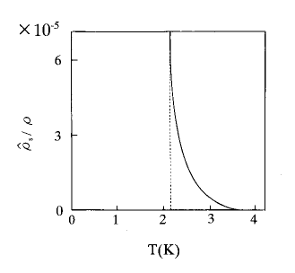
Figure 5: $\hat{\rho}_{s}(T)/\rho$ obtained by Eq.(45) using $\nu(T)$ in Fig.1.

In the rotation experiment by Hess and Fairbank hes , the moment of inertia $I_{z}$ just above $T_{\lambda}$ is slightly smaller than the normal phase value $I_{z}^{cl}$ (see Sec.6.A). Using these currently available data, Ref.koh roughly estimates $\hat{\rho}_{s}(T)/\rho$ as $\hat{\rho_{s}}(T_{\lambda}+0.03K)/\rho\cong 8\times 10^{-5}$, and $\hat{\rho_{s}}(T_{\lambda}+0.28K)/\rho\cong 3\times 10^{-5}$. Although the precision of these estimates is limited, the agreement of $\hat{\rho}_{s}(T)/\rho$ in Fig.5 with these values is good beyond our expectation.

(2) In Sec.4, we obtained the interpolation formula for $\hat{\rho}_{s}(T)/\rho$, Eq.(36). We assume $\mu-\Sigma$ changes with temperature according to the formula

$$\mu(T)-\Sigma(U)=-\left(\frac{g_{3/2}(1)}{2\sqrt{\pi}}\right)^{2}k_{B}T_{\lambda}\left[\left(\frac{T}{T_{\lambda}}\right)^{3/2}-1\right]^{2},$$ (46)

($g_{a}(x)=\sum_{n}x^{n}/n^{a}$). Here we assume that the particle interaction $U$ and the particle density $\rho$ of liquid helium 4 are renormalized to $T_{\lambda}=2.17K$, which is an approximation that dates back to London. Equation.(36) with Eq.(46) predicts a temperature dependence of $\hat{\rho}_{s}(T)/\rho$. Although it bears a qualitative resemblance to $\hat{\rho}_{s}(T)/\rho$ in Fig.5, it differs from Fig.5 in that $\hat{\rho}_{s}(T)/\rho$ in Eq.(36) remains very small at $3.7K>T>2.3K$ $(=T_{\lambda}+0.2K)$, but it abruptly increases at 2.3K, and reaches a macroscopic number at $T_{\lambda}$, thus resembling the shape of the letter $L$. Experimentally, as temperature decreases from 3.7K to $T_{\lambda}$, $\hat{\rho}_{s}(T)/\rho$ gradually increases as in Fig.5. This means that Eq.(36) and the approximation behind it is too simple to be compared quantitatively to the real system. With decreasing temperature, in addition to the particle with $p=0$, other particles having small but finite momenta get to contribute to the $1/q^{2}$ divergence of $\hat{\chi}_{\mu\nu}(q,0)$ as well. (In addition to Eq.(30), a new $F_{\beta}(q,0)$ including $p\neq 0$ also satisfies $1-UF_{\beta}(0,0)=0$ in Eq.(29).) Hence, the total $\hat{\rho_{s}}(T)$ is a sum of each $\hat{\rho_{s}}(T)$ over different momenta den . The participation of $p\neq 0$ particles into $\hat{\rho_{s}}(T)$ is a physically natural phenomenon. For the repulsive Bose system, particles are likely to spread uniformly in coordinate space due to the repulsive force. This feature makes the particles with $p\neq 0$ behave similarly with other particles, especially with the particle having zero momentum. If they move at different velocities along the flow direction, the particle density becomes locally high, thus raising the interaction energy. This is the reason why many particles with $p\neq 0$ participate in the superfluid flow even if it is just above $T_{\lambda}$ .

(3) Equations (35) and (46) with $T_{on}=3.7K$ gives us a rough estimate of $U$ as $U\sim 3.4\times 10^{-16}erg$. This value is approximately close to $U_{s}\cong\hbar^{2}/(ma^{2})=3.4\times 10^{-17}$ $erg$ derived from the scattering length $a=0.7$ $nm$, which is based on the sound velocity $v_{s}=220$ $m/s$ and the Bogoliubov formula $v_{s}=(\hbar/m)\sqrt{4\pi na}$. But this $U$ is somewhat larger than $U_{s}$.

VI Discussion

VI.1 Superfluidity in the non-dissipative and the dissipative flows

On the onset mechanism of superfluidity, there are physical differences between the non-dissipative and the dissipative flows.

As an example of the non-dissipative flow, we considered the flow in a rotating bucket in Sec.2, in which the quantity directly indicating the onset of superfluidity is the moment of inertia

$$I_{z}=I_{z}^{cl}\left(1-\frac{\hat{\rho_{s}}(T)}{\rho}\right),$$ (47)

where $I_{z}^{cl}$ is its classical value.

(1) $I_{z}$ of a superfluid consists only of a linear term of $I_{z}^{cl}$, and $\hat{\rho_{s}}(T)$ appears as a correction to its coefficient.

(2) The change of $\chi^{L}-\chi^{T}$ directly affects $I_{z}$ without being enhanced, and therefore just above $T_{\lambda}$, the effect of a small but finite $\hat{\rho_{s}}(T)$ on $I_{z}$ is small koh .

For the dissipative flow, we considered the capillary flow, in which the quantity directly indicating the onset of superfluidity is the shear viscosity. Comparing Eq.(25) to Eq.(47), we note the following features in $\nu(T)$.

(1) $\nu(T)$ of a superfluid has a form of an infinite power series of $\nu_{n}$, and the influence of Bose statistics appears in all coefficients of higher-order terms except for the first-order one. This feature does not depend on a particular model of a liquid, but on the general argument. (On the other hand, the microscopic derivation of the value of $\nu_{n}$ depends on the model of a liquid, which is a subject of the liquid theory and beyond the scope of this paper.)

(2) Because of the emergence of the sharp peak due to Eq.(22) in the dispersion integral, a small change of $\hat{\rho_{s}}(T)$ is strongly enhanced to an observable change of $\nu(T)$ in Eq.(25).

(3) The existence of $1/d^{2}$ in front of $\hat{\rho_{s}}(T)/\rho$ in the denominator of Eq.(25) indicates that a narrower capillary shows a clearer evidence of a frictionless flow. Similarly, the existence of $1/\omega_{e}$ indicates that the choice of experimental procedure such as the method of applying the pressure to both ends of the capillary affects the temperature dependence of $\nu(T)$ of the capillary flow. This means that the dissipative phenomena depend on more variables than the non-dissipative ones.

VI.2 Comparison to thermal conductivity

There is another type of significant change of conductivity in liquid helium 4, an anomalous thermal conductivity at $T<T_{\lambda}$. Under a given temperature gradient $\nabla T$, a heat flow $q$ satisfies $q=-\kappa\nabla T$, where $\kappa$ is the coefficient of thermal conductivity. In the critical region above $T_{\lambda}$ ($T/T_{\lambda}-1<10^{-3}$), the rapid rise of $\kappa$ is observed, and finally at $T=T_{\lambda}$, $\kappa$ jumps to an at least $10^{7}$ times higher value kel . (This rise is a subject of the fluctuation theory of liquid helium 4 pha .) Comparing to $\eta(T)$ which shows a symptom of its fall in $T_{\lambda}<T<3.7K$, $\kappa(T)$ does not show a symptom of its rise in the same temperature region.

The coefficient of thermal conductivity has a formally similar structure of correlation function to that of the shear viscosity, but they are qualitatively different phenomena. While shear viscosity is associated with the transport of momentum (a vector), thermal conductivity is associated with that of energy (a scalar). For the vector field (velocity field), the direction of vectors has a huge number of possibilities in its spatial distribution. Hence, among various flow-velocity fields, we can regard the flow in a rotating bucket as a non-dissipative counterpart to the capillary flow. On the other hand, for the scalar field (temperature field), the variety of possible spatial distributions is far limited. A heat flow is always a dissipative phenomenon, and there is no non-dissipative counterpart. Hence, to the onset of the anomalous thermal conductivity, the mechanism that amplifies the small $\hat{\rho_{s}}(T)$ to an observable change cannot be applied. This formal difference between shear viscosity and thermal conductivity is consistent with the experimental difference between $\eta(T)$ and $\kappa(T)$ at $T_{\lambda}<T<3.7K$.

VI.3 Comparison to Fermi liquids

The fall of the shear viscosity in liquid helium 3 at $T_{c}$ is a parallel phenomenon to that in liquid helium 4. The formalism in Sec.2 and 3 is applicable to liquid helium 3 as well. For the behavior above $T_{c}$, however, there is a striking difference between liquid helium 3 and 4. The phenomenon occurring in fermions in the vicinity of $T_{c}$ is not a gradual growth of the coherent wave function, but a formation of the Cooper pairs by two fermions. (This difference evidently appears in the temperature dependence of the specific heat: $C(T)$ of liquid helium 3 shows only a sharp peak at $T_{c}$, and does not show a symptom of its rise above $T_{c}$.) Once the Cooper pairs are formed, they are composite bosons with high density at low temperature, and immediately jumps to the superfluid state. Hence, the shear viscosity of liquid helium 3 shows an abrupt drop at $T_{c}$ without a gradual fall above $T_{c}$.

In electron superconductivity, there is an energy gap due to the formation of Cooper pairs. Hence, in its conductivity spectrum $\sigma(\omega)$ at $T<T_{c}$, there is a frequency gap $\omega_{g}$ near $\omega=0$ flu . In superfluid helium 4, due to the acoustic phonon, there is no energy gap, which is consistent with that $\sigma_{n}(\omega)$ in Eq.(43) is a weakly $\omega$-dependent function.

Appendix A $h(t)=h(0)\exp(-\alpha t)$

The mass of a liquid passing through a capillary per unit time is $Q=2\pi\rho\int_{0}^{d}rv_{z}(r)dr$, which is determined by Eq.(3) as

$$Q=\rho\frac{\pi d^{4}}{8\eta}\frac{\Delta P}{L}.$$ (48)

The mass of a liquid in the reservoir with a radius $R$, $\rho\pi R^{2}h(t)$, flows out through a capillary at the rate of $Q$. The pressure at the upper and lower end of the capillary set up vertically is $1+\rho gh$ and $1$ atm, respectively, thus leading to $\Delta P(t)=\rho gh(t)$ in Eq.(A1). The level $h(t)$ of the liquid in the reservoir decreases according to

$$\rho\pi R^{2}\frac{dh}{dt}=-\frac{\pi d^{4}}{8\eta}\frac{\rho^{2}g}{L}h,$$ (49)

thereby leading to $h(t)=h(0)\exp(-\alpha t)$ with $\alpha=\rho gd^{4}/(8\eta LR^{2})$. For liquid helium 3, $\rho/\eta$ in $\alpha$ is $3.6\times 10^{3}$ at $T=1.1K$, and $3.8\times 10^{3}$ at $T=3.0K$. For liquid helium 4, $\rho/\eta$ is $4.2\times 10^{3}$ at $T=3.0K$.

Appendix B Conductivity spectrum $\sigma(\omega)$

The Stokes equation under the oscillatory pressure gradient $\Delta Pe^{i\omega t}/L$ is written in the cylindrical polar coordinate as follows

$$\frac{\partial v}{\partial t}=\nu\left(\frac{\partial}{\partial r^{2}}+\frac{\partial}{r\partial r}\right)v+\frac{\Delta Pe^{i\omega t}}{\rho L}.$$ (50)

The velocity has the following form

$$v(r,t)=\frac{\Delta Pe^{i\omega t}}{i\omega\rho L}+\Delta v(r,t),$$ (51)

under the boundary condition $v(d,t)=0$. In Eq.(B1), $\Delta v(r,t)$ satisfies

$$\frac{\partial\Delta v(r,t)}{\partial t}=\nu\left(\frac{\partial}{\partial r^{2}}+\frac{\partial}{r\partial r}\right)\Delta v(r,t),$$ (52)

and therefore $\Delta v(r,t)$ has a solution written in terms of the Bessel function $J_{0}(i\lambda r)$ with $\lambda=(1+i)\sqrt{\omega/(2\nu)}$. Hence,

$$v(r,t)=\frac{\Delta Pe^{i\omega t}}{i\omega\rho L}\left(1-\frac{J_{0}(i\lambda r)}{J_{0}(i\lambda d)}\right).$$ (53)

Using Eq.(B4) at $r=0$, the conductivity spectrum $\sigma(\omega)$, which is defined by Eq.(6) as $\rho v(0,t)=\sigma(\omega)d^{2}\Delta Pe^{i\omega t}/L$, is given by

$$\sigma(\omega)=\frac{1}{i\omega d^{2}}\left(1-\frac{1}{J_{0}\left(id[1+i]\displaystyle{\sqrt{\frac{\omega}{2\nu}}}\right)}\right).$$ (54)

The real part of Eq.(B5)

$$Re\sigma(\omega)=\frac{1}{\omega d^{2}}\frac{\displaystyle{\sum_{n=0}^{\infty}\frac{1}{(n!)^{2}}}\left(\frac{\omega d^{2}}{4\nu}\right)^{n}\cos\frac{n\pi}{2}}{\displaystyle{\left[\sum_{n=0}^{\infty}\frac{1}{(n!)^{2}}\left(\frac{\omega d^{2}}{4\nu}\right)^{n}\cos\frac{n\pi}{2}\right]^{2}}+\displaystyle{\left[\sum_{n=0}^{\infty}\frac{1}{(n!)^{2}}\left(\frac{\omega d^{2}}{4\nu}\right)^{n}\sin\frac{n\pi}{2}\right]^{2}}}.$$ (55)

gives a curve of $\sigma(\omega)$ in Fig.3(a). (Re $\sigma(0)$ in Eq.(B5) agrees with $\rho/(4\eta)$.) Furthermore, it determines the conserved quantity $f(d)\propto d^{-2}$ in Eq.(7). ($\nu$ in Eq.(B5) disappears in $\int\sigma(\omega)d\omega$.)

Appendix C Flow in a rotating bucket

The hamiltonian of a liquid in a coordinate system rotating with the container is $H-\mbox{\boldmath$\Omega$}\cdot\mbox{\boldmath$L$}$, where $L$ is the total angular momentum. The perturbation $H_{ex}=-\mbox{\boldmath$\Omega$}\cdot\mbox{\boldmath$L$}$ is cast in the form $-\sum_{i}(\mbox{\boldmath$\Omega$}\times\mbox{\boldmath$r$})\cdot\mbox{\boldmath$p$}$ , in which $\mbox{\boldmath$\Omega$}\times\mbox{\boldmath$r$}\equiv\mbox{\boldmath$v$}_{d}(\mbox{\boldmath$r$})$ serves as an external field. The rotation is equivalent to the application of the external field. We define the mass-flow density $\mbox{\boldmath$j$}(\mbox{\boldmath$r$})$ in the rotation, and express the perturbation $H_{ex}$ as

$$-\mbox{\boldmath$\Omega$}\cdot\mbox{\boldmath$L$}=-\int\mbox{\boldmath$v$}_{d}(\mbox{\boldmath$r$})\cdot\mbox{\boldmath$j$}(\mbox{\boldmath$r$})d^{3}x.$$ (56)

Because of $div\mbox{\boldmath$v$}_{d}(\mbox{\boldmath$r$})=0$, $\mbox{\boldmath$v$}_{d}(\mbox{\boldmath$r$})$ in Eq.(C1) acts as a transverse-vector probe to the excitation of bosons. This fact allows us a formal analogy that the response of the system to $\mbox{\boldmath$v$}_{d}(\mbox{\boldmath$r$})$ is analogous to the response of the charged Bose system to the vector potential $\mbox{\boldmath$A$}(\mbox{\boldmath$r$})$ in the Coulomb gauge. Hence, in momentum space, $\mbox{\boldmath$j$}(\mbox{\boldmath$r$})$ in Eq.(C1) has the following microscopic form similar to that in the charged Bose system

$$j_{\mu}(q,\tau)=\sum_{p,n}\left(p+\frac{q}{2}\right)_{\mu}\Phi_{p}^{\dagger}\Phi_{p+q}e^{-i\omega_{n}\tau},$$ (57)

($\hbar=1$ and $\tau=it$).

Appendix D Maxwell’s relation

Consider the shear deformation of a solid and of a liquid. In a solid, shear stress $F_{xy}$ is proportional to a shear angle $\phi$ as $F_{xy}=G\phi$, where $G$ is the modulus of rigidity. The value of $G$ is determined by dynamical processes in which vacancies in a solid move to neighboring positions over the energy barriers. As $\phi$ increases, $F_{xy}$ increases as follows,

$$\frac{dF_{xy}}{dt}=G\frac{d\phi}{dt}.$$ (58)

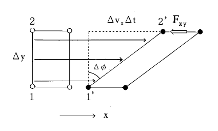
Figure 6: In a liquid flowing along the $x$-direction, owing to the velocity gradient along the $y$-direction, a small rectangular part of a liquid is deformed to a parallelogram.

In a liquid, the situation is different as follows. Figure 6 represents a small portion of the flow in Fig.2, in which two particles 1 and 2, each of which starts at $(x,y)$ and $(x,y+\Delta y)$ simultaneously, moves along the $x$-direction. In a liquid, the relative position of particles is not rigid, but with the flow motion it changes so as to reduce the shear stress $F_{xy}$ between adjacent layers. Presumably, the larger shear stress induces the faster structural relaxation, that is, the rate of such relaxations is proportional to the magnitude of $F_{xy}$. Hence, instead of Eq.(D1), one obtains

$$\frac{dF_{xy}}{dt}=G\frac{d\phi}{dt}-\frac{F_{xy}}{\tau_{st}},$$ (59)

where $\tau_{st}$ is a relaxation time. In the stationary flow after relaxation, $F_{xy}$ remains constant, and one obtains

$$G\frac{d\phi}{dt}=\frac{F_{xy}}{\tau_{st}}.$$ (60)

Assume that there is velocity gradient $v_{x}(y)$ along $y$ direction in Fig.6. After $\Delta t$ has passed, they (1’ and 2’) are at a distance of $\Delta v_{x}\Delta t$ along the $x$-direction. The shear angle increases from zero to $\Delta\phi$, which satisfies $\Delta v_{x}\Delta t=\Delta y\Delta\phi$ as depicted in Fig.6. Hence, we obtain

$$\frac{\partial v_{x}}{\partial y}=\frac{d\phi}{dt}.$$ (61)

Substituting Eq.(D4) into Eq.(D3), and comparing it with Eq.(1), one obtains $\eta=G\tau_{st}$ (Maxwell’s relation).

References

- (1) P.Kapitza, Nature.141, 74(1938), J.F.Allen and A.D.Misener, Nature.141, 75(1938)
- (2) R.Bowers and K.Mendelssohn, Proc.Roy.Soc.Lond.A.204, 366(1950). They pointed out that the fall of above did not come from thermal fluctuations.
- (3) H.Tjerkstra, Physica.19, 217(1953)
- (4) K.N.Zinoveva, Zh.Eksp.Teor.Fiz.34, 609(1958) [Sov.Phys-JETP.7, 421(1958)]
- (5) C.F.Barenghi, P.J.Lucas, and R.J.Donnelly, J.Low.Temp.Phys.44, 491(1981)
- (6) A.Z.Patashinskii and V.L.Pokrovskii, J.Exptl.Theoret.Phys.(USSR)46, 994(1964) [Sov.Phys-JETP.19, 677(1964)], R.A.Farrell, N.Menyhard, H.Schmidt, F.Schwabl and P.Szepfalusy, Ann.Phys. 47, 565(1968), B.I.Halperin and P.C.Hoenberg, Phy.Rev.177, 952(1969). T.Tsuzuki, Prog.Theor.Phys.41, 1387(1969), I.M.Khalatnikov, Zh.Eksp.Teor.Fiz.57, 489(1969) [Sov.Phys-JETP.30, 268(1970)], A.M.Polyakov, Zh.Eksp.Teor.Fiz.57, 2144(1969) [Sov.Phys-JETP.30, 1164(1970)]. The superfluid density is influenced by the phase fluctuation of the order parameter, which only slightly differs from the conventional within the range of .
- (7) The increase of by the critical slowing down is negligible at .
- (8) The fluctuation-dissipation theorem is not applicable to the non-dissipative response such as the onset of superfluidity.
- (9) F.London Superfluid, John Wiely and Sons, New York, 1954 Vol.2, 141.
- (10) S.Koh, Phy.Rev.B.74, 054501(2006).
- (11) L.D.Landau and I.M. Khalatonikov, Zh.Eksp.Teor.Fiz.19, 637, 709(1949), in Collected papers of L.D.Landau, (edited by D.ter.Haar, Pergamon, London, 1965).
- (12) J.M.Goodwin, PhD Thesis, University of Washington (1968)
- (13) B.Welber, Phy.Rev.119, 1816(1960), B.Welber and D.C.Hammer, Phys.Lett.15, 233(1965), B.Welber and G.Allen, Phys.Lett.33A, 213(1970).
- (14) L.Bruschi, G.Mazzi, M.Santini and G.Torzo, J.Low.Temp.Phys.29, 63(1977)
- (15) G.B.Hess and W.M.Fairbank, Phy.Rev.19, 216(1967)
- (16) In the short time scale, the mechanism of the shear viscosity in a liquid is similar to that in a solid, and is therefore a highly inhomogeneous process at the molecular level: The modulus of rigidity is determined by the motion of vacancy as in a solid.
- (17) L.P.Kadanoff and P.C.Martin, Ann.Phys. 24, 419(1963).
- (18) As a text, L.D.Landau and E.M.Lifshitz, Fluid Mechanics, 2nd ed, (Pergamon Press, 1987).
- (19) As a response to , at another point is possible, but it results in the same form of .
- (20) Using Eq.(2), of model is calculated beyond the one-loop level in the context of the relativistic heavy ion collision by S.Jeon, Phy.Rev.D.52, 3591(1995), E.Wang and U.Heinz, Phys.Lett.B. 52, 208(1999). These results describe the shear viscosity of a strongly interacting dense gas. For a liquid, however, the anisotropic particle interaction with the hard core must be introduced in calculations.
- (21) R.Kubo, J.Phys.Soc.Japan.12, 570(1957). Equation (7) is an oscillator-strength sum rule in terms of fluid conductivity through a capillary.
- (22) Just after the advent of BCS model, an attempt was made to relate the electrical conductivity (more precisely, the micro-wave absorption spectrum) with the penetration depth in the Meissner effect by R.A.Ferrell and R.E.Glover, Phy.Rev.109, 1398(1958), and by M.Tinkham and R.A.Ferrell, Phy.Rev.2, 331(1959). (As a text, M.Tinkham Introduction to superconductivity, 2nd ed, (McGraw-Hill, New York, 1996)). Whereas the electrical conduction is a dissipative phenomenon, the Meissner effect is a non-dissipative one, and is an analogue to the nonclassical fluid flow in a rotating bucket noz .
- (23) In Ref fer , the definition of the vector potential plays the role of Eq.(9).
- (24) in the right-hand side of Eq.(10) is a fictitious velocity that appears when the system would obey Eq.(9) for the non-interacting system, whereas in of the left-hand side is a real velocity in the interacting system.
- (25) As a review, P.Nozieres, in Quantum Fluids (ed by D.E.Brewer), 1 (North Holland, Amsterdam, 1966), G.Baym, in Mathematical methods in Solid State and Superfluid Theory (ed by R.C.Clark and G.H.Derrick), 121 (Oliver and Boyd, Edingburgh, 1969)
- (26) J.C.Maxwell, Phil.Trans.Roy.Soc.157, 49(1867) in The scientific papers of J.C.Maxwell, (edited by W.D.Niven, Dover, New York, 2003) Vol.2, 26.
- (27) We usually use the density , a longitudinal susceptibility satisfying , for the transverse response of the system as in the conductivity . This is explained by the replaceability of by in Eq.(19).
- (28) E.C.Kerr, J.Chem.Phys.26, 511(1957), and E.C.Kerr and R.D.Taylor, Ann.Phys. 26, 292(1964).
- (29) In a classical liquid, is inversely proportional to the rate of processes in which vacancies in a liquid propagate from one point to another over the energy barriers. With decreasing temperature, this rate decreases. The liquid therefore slowly respond to perturbations, and its increases.
- (30) R.P.Feynman, in Progress in Low Temp Phys. 1, (ed C.J.Gorter), 17 (North-Holland, Amsterdam, 1955).
- (31) The structural characteristic of liquids is irregular arrangements of molecules, the energies of which and differ only slightly to each other. In the relaxation from one of these arrangements to others, the small leads to the long of a classical liquid.
- (32) In the strong-coupling system, however, the strong interaction disturbs the relaxation, thereby leading to a large .
- (33) It is possible that a more complex diagram than a bubble exchanges particles with the tensor . While it is difficult to estimate an infinite sum of these diagrams, it adds only a small correction.
- (34) R.P.Feynman, Phy.Rev.91, 1291(1953).
- (35) The stability of a superfluid has been studied in the context of the critical velocity of the persistent current. Above , the system is unstable, and changes to a state with a topologically different structure of order parameter. On the other hand, the stability concerning is a more primitive one in the growth process of the coherent wave function. (As a review, J.S.Langer and J.D.Reppy, in Progress in Low Temp Phys. 6, (ed C.J.Gorter), ch.1 (North-Holland, Amsterdam, 1970).)
- (36) L.D.Landau, J.Phys.USSR.5, 71(1941).
- (37) The at in Fig.5 is a completely different concept from the fluctuation-driven superfluid density, which was proposed in Ref.pha at .
- (38) The density of states for this sum is not proportional to but a constant, because it is owing to the one-dimensional momenta along the flow.
- (39) L.J.Challis and J.Wilks, in Proceedings of the Symposium on Solid and Liquid (Ohio State University, Ohio, 1957). J.F.Kerrisk and W.E.Keller, Phy.Rev.177, 341(1969).
- (40) In electron superconductors, in addition to the normal conductivity , an extra () is observed at , which is considered to be driven by fluctuations.