Regular projections of graphs with at most three double points

Abstract.

A generic immersion of a planar graph into the 2-space is said to be knotted if there does not exist a trivial embedding of the graph into the 3-space obtained by lifting the immersion with respect to the natural projection from the 3-space to the 2-space. In this paper we show that if a generic immersion of a planar graph is knotted then the number of double points of the immersion is more than or equal to three. To prove this, we also show that an embedding of a graph obtained from a generic immersion of the graph (does not need to be planar) with at most three double points is totally free if it contains neither a Hopf link nor a trefoil knot.

1. Introduction

Throughout this paper we work in the piecewise linear category and graphs are considered as topological spaces. Let ${\mathbb{S}}^{3}$ be the unit $3$-sphere in ${\mathbb{R}}^{4}$ centered at the origin. For a finite graph $G$, an embedding $f:G\to{\mathbb{S}}^{3}$ is called a spatial embedding of $G$ or simply a spatial graph. If $G$ is homeomorphic to the disjoint union of $n$ circles, then $f$ is called an $n$-component link (or a knot if $n=1$). Two spatial embeddings $f$ and $g$ of $G$ are said to be equivalent ($f\approx g$) if there exists an orientation-preserving self-homeomorphism $\Phi$ on ${\mathbb{S}^{3}}$ such that $\Phi(f(G))=g(G)$. A graph $G$ is said to be planar if there exists an embedding of $G$ into the unit $2$-sphere ${\mathbb{S}}^{2}$. A spatial embedding of a planar graph $G$ is said to be trivial if it is equivalent to an embedding $h:G\to{\mathbb{S}}^{2}\subset{\mathbb{S}}^{3}$.

A continuous map $\varphi:G\to{\mathbb{S}}^{2}$ is called a regular projection of $G$ if the multiple points of $\varphi$ are only finitely many transversal double points away from the vertices of $G$. For a spatial embedding $f$ of $G$, we also say that $\varphi$ is a regular projection of $f$ or $f$ projects on $\varphi$, if there exists an embedding $f^{\prime}:G\to{\mathbb{S}}^{3}\setminus\left\{(0,0,0,1),(0,0,0,-1)\right\}$ such that $f$ is equivalent to $f^{\prime}$ and $\pi\circ f^{\prime}=\varphi$, where $\pi:{\mathbb{S}}^{3}\setminus\left\{(0,0,0,1),(0,0,0,-1)\right\}\to{\mathbb{S}}^{2}$ is the natural projection, see Fig. 1.1. A regular diagram $\widetilde{\varphi}$ of $f$ is none other than the regular projection $\varphi$ of $f$ with over/under information of each double point. We call a double point with over/under information a crossing. For a subspace $H$ of $G$, we often denote $\varphi(H)$ (resp. $\widetilde{\varphi}(H)$) by $\widehat{H}$ (resp. $\widetilde{H}$) as long as no confusion occurs.

Figure 1.1.

Our purpose in this paper is to investigate knotted projections which realize the minimal number of double points. A regular projection $\varphi$ of a planar graph $G$ is said to be knotted if there does not exist any trivial spatial embedding of $G$ which projects on $\varphi$. Such a regular projection was discovered by K. Taniyama first [11]. For example, let $\varphi$ be the regular projection illustrated in Fig. 1.2. Then we can see that any spatial embedding of $G$ which projects on $\varphi$ contains a Hopf link, so $\varphi$ is knotted. We call a knotted regular projection simply a knotted projection. By the notion of knotted projection, a problem in graph minor theory can be formulated [3]. A planar graph is said to be trivializable if it has no knotted projections. Let $\Omega$ be the set of all non-trivializable planar graphs whose all proper minors are trivializable. It is known that for any trivializable planar graph $G$ every minor of $G$ is also trivializable [11]. Therefore, due to the celebrated work of Robertson and Seymour on graph minors [6], it is guaranteed that $\Omega$ is finite. But, although many elements of $\Omega$ have been found out through continued works [9, 10, 4, 5], the set is not completely determined yet. In this paper, as an effort on this issue, we will give necessary conditions for knotted projections.

Figure 1.2.

Let $d$ be a double point of a regular projection $\varphi$ of $G$ such that $\varphi^{-1}(d)=\left\{p_{1},p_{2}\right\}$ and $p_{i}\in e_{i}$, where $e_{i}$ is an edge of $G$ ($i=1,2$). Then we say that $d$ is Type-S if $e_{1}=e_{2}$, Type-A if $e_{1}\neq e_{2}$ and $e_{1}\cap e_{2}\neq\emptyset$, and Type-D if $e_{1}\cap e_{2}=\emptyset$. Then we have the following. Here we denote the number of all double points of a regular projection $\varphi$ by ${\rm cr}(\varphi)$. And a regular projection of a planar graph $G$ is said to be trivial if only trivial spatial embeddings of $G$ project on it

Theorem 1-1.

Let $\varphi$ be a regular projection of a planar graph $G$. Then we have the following.

1. If ${\rm cr}(\varphi)=1$, then $\varphi$ is trivial.

2. If ${\rm cr}(\varphi)=2$, then $\varphi$ is not knotted. Moreover, $\varphi$ is trivial if $\varphi$ has a double point of Type-S or Type-A.

3. If ${\rm cr}(\varphi)=3$, then $\varphi$ is not knotted if $\varphi$ has a double point of Type-S or Type-A.

As a corollary of Theorem 1-1, necessary conditions for knotted projections are derived.

Corollary 1-2.

If a regular projection $\varphi$ of a planar graph is knotted, then ${\rm cr}(\varphi)\geq 3$. In partcular, if $\varphi$ is knotted and ${\rm cr}(\varphi)=3$ then every double point of $\varphi$ is Type-D.

As we saw in Fig. 1.2, there exists a knotted projection with only three double points. Thus the inequality of Corollary 1-2 is best possible.

To accomplish the proof of Theorem 1-1, we determine non-trivial spatial graph types which may be contained in a spatial embedding of a graph which projects on a regular projection of the graph with at most three double points. In the case of an $n$-component link $L$ which projects on a regular projection with at most three double points, it is not hard to see in knot theory that $L$ is trivial if it does not contain a Hopf link or a trefoil knot. In the following we generalize the above fact to spatial graphs. A spatial embedding $f$ of a graph $G$ is said to be free if the fundamental group of the spatial graph complement $\pi_{1}({\mathbb{S}}^{3}\setminus f(G))$ is free. Moreover we say that $f$ is totally free if the restriction map $f|_{H}$ is free for any subgraph $H$ of $G$. For example, the two spatial graphs in Fig. 1.3 are free but not totally free. We remark here that if $G$ is planar, then $f$ is totally free if and only if $f$ is trivial by Scharlemann-Thompson’s famous theorem [8]. Then we have the following.

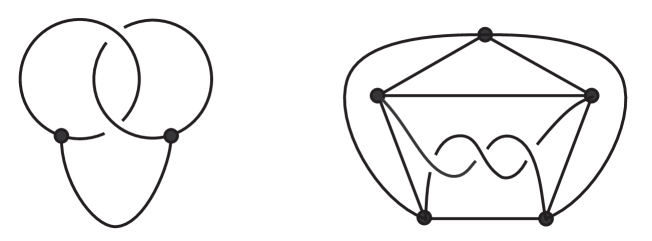
Figure 1.3.

Theorem 1-3.

Let $\varphi$ be a regular projection of a graph $G$ and $f$ a spatial embedding of $G$ which projects on $\varphi$. Assume that ${\rm cr}(\varphi)\leq 3$. Then $f$ is totally free if it does not contain a Hopf link or a trefoil knot.

As a direct consequense of Theorem 1-3, we have the following corollary.

Corollary 1-4.

Let $\varphi$ be a regular projection of a planar graph $G$ and $f$ a spatial embedding of $G$ which projects on $\varphi$. Then we have the following.

1. If ${\rm cr}(\varphi)=1$, then $f$ is trivial.

2. If ${\rm cr}(\varphi)=2$, then $f$ is trivial if it does not contain a Hopf link.

3. If ${\rm cr}(\varphi)=3$, then $f$ is trivial if it does not contain a Hopf link or a trefoil knot.

Corollary 1-4 also leads to another fundamental result on spatial graphs. A spatial embedding $f$ of a planar graph $G$ is said to be minimally knotted if $f$ is not trivial but $f|_{H}$ is trivial for any proper subgraph $H$ of $G$. Fig. 1.1 shows an example of minimally knotted spatial embedding which is called Kinoshita’s theta curve. Note that every planar graph without isolated vertices and free vertices has minimally knotted spatial embeddings [2, 14].

Corollary 1-5.

Let $\varphi$ be a regular projection of a planar graph $G$ and $f$ a minimally knotted spatial embedding of $G$ which projects on $\varphi$. If $f$ is neither a Hopf link nor a trefoil knot, then ${\rm cr}(\varphi)\geq 4$.

Proof.

If ${\rm cr}(\varphi)\leq 3$, by Theorem 1-3 we have that $f$ contains a Hopf link or a trefoil knot. Since $f$ is minimally knotted, $f$ must be a Hopf link or a trefoil knot. ∎

The inequality of Corollary 1-5 is best possible. For example, the spatial handcuff graph in Fig. 1.4 is minimally knotted and it can project on a regular projection with four double points.

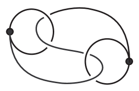
Figure 1.4.

By Corollary 1-5, we also give a partial answer for Ozawa’s question [4, Question 3.7] which asks whether a minimally knotted spatial embedding of a planar graph can project on a knotted projection of the graph or not.

Corollary 1-6.

Let $\varphi$ be a knotted projection of a planar graph $G$ with ${\rm cr}(\varphi)=3$. Then there does not exist a minimally knotted spatial embedding of $G$ which projects on $\varphi$.

Remark 1-7.

There exists a regular projection $\varphi$ of a non-planar graph $G$ with ${\rm cr}(\varphi)=2$ such that no totally free spatial embeddings of $G$ project on $\varphi$. For example, let $\varphi$ be the regular projection of a non-planar graph $G$ as illustrated in Fig. 1.5. Then we can see that any of the spatial embedding of $G$ which projects on $\varphi$ contains a Hopf link [12, Fig. 4]. This says that the planarity of a graph is essential in Theorem 1-1.

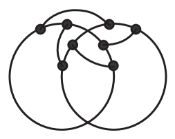
Figure 1.5.

The rest of this paper is organized as follows. In the next section, we introduce a key theorem which is needed to prove our theorems. We prove Theorem 1-3 in section 3. And, by utilizing the theorem, the proof of Theorem 1-1 is given in section 4.

2. Key theorem

To prove Theorem 1-3 and 1-1, we take advantage of a nice geometric characterization of totally free spatial embeddings which was first proved by Wu for planar graphs [13, THEOREM 2] and generalized to arbitrary graphs (not need to be planar) by Robertson-Seymour-Thomas [7, (3.3)]. Here a cycle of a graph $G$ is a subgraph of $G$ which is homeomorphic to the circle, and a disk is a topological space which is homeomorphic to the unit $2$-disk ${\mathbb{D}}^{2}$ in ${\mathbb{R}}^{2}$.

Theorem 2-1.

[7, (3.3)] A spatial embedding $f$ of a graph $G$ is totally free if and only if for any cycle $\gamma$ of $G$ there exists a disk $D_{\gamma}$ in ${\mathbb{S}}^{3}$ such that

$$f(G)\cap D_{\gamma}=f(G)\cap\partial D_{\gamma}=f(\gamma).$$

Namely $f$ is totally free if and only if for any cycle $\gamma$ of $G$ the knot $f(\gamma)$ bounds a disk $D_{\gamma}$ in ${\mathbb{S}}^{3}$ as a Seifert surface such that ${\rm int}D_{\gamma}\cap f(G)=\emptyset$. We call $D_{\gamma}$ a trivialization disk for $f(\gamma)$. Theorem 2-1 helps us to detect the totally freedom (or triviality) of a spatial graph by utilizing local informations in the regular diagram.

To put it into practice, we introduce some definitions. Let $\widetilde{\varphi}$ be a regular diagram of a spatial embedding of a graph $G$. Fix a cycle $\gamma$ of $G$. Among the edges of $G$ not contained in $\gamma$, choose all possible edges $e_{1},e_{2},\ldots,e_{m}$ so that $\widehat{\gamma}$ and $\widehat{e}_{i}$ produce double points of $\varphi$. We denote the subgraph of $G$ which is obtained from $G$ by forgetting $e_{1},e_{2},\ldots,e_{m}$ by $G^{\prime}$. Let $R_{1},R_{2},\ldots,R_{k}$ be all of the connected components of ${\mathbb{S}}^{2}\setminus\widehat{\gamma}$. We denote the subspace $\varphi^{-1}\left(\widehat{G^{\prime}}\cap R_{i}\right)$ of $G^{\prime}$ by $H_{i}\ (i=1,2,\ldots,k)$.

For example, given a regular diagram as the left-hand side of Fig. 2.1, let $\gamma$ be the cycle of $G$ such that $\widetilde{\gamma}$ corresponds to the gray curve in the center of Fig. 2.1, where $\widetilde{e}_{1}$ and $\widetilde{e}_{2}$ are drawn by dotted black lines. Then the right-hand side of Fig. 2.1 illustrates $\widetilde{H}_{1},\widetilde{H}_{2}$ and $\widetilde{H}_{3}$. We often describe such circumstances around $\widetilde{\gamma}$ (resp. $\widehat{\gamma}$) by thumbnailing each $\widetilde{H}_{i}$ (resp. $\widehat{H}_{i}$) with the ends as illustrated in Fig. 2.2. We define the interferency of $\widehat{\gamma}$ as the number of all double points on $\widehat{\gamma}$ in $\widehat{G}$ which are not self double points of $\widehat{\gamma}$.

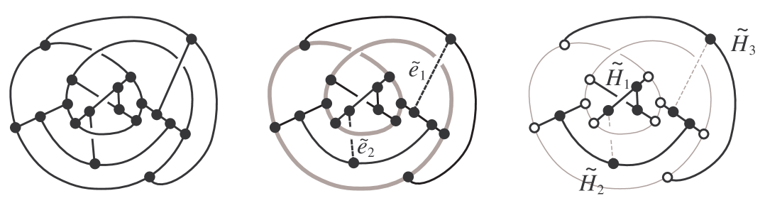
Figure 2.1.

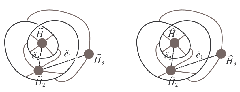
Figure 2.2.

3. Proof of Theorem 1-3

First we give two lemmas necessary for the proof of Theorem 1-3.

Lemma 3-1.

Let $\varphi$ be a regular projection of a graph $G$, $f$ a spatial embedding of $G$ which projects on $\varphi$ and $\gamma$ a cycle of $G$. If $\varphi|_{\gamma}$ is trivial and the interferency of $\widehat{\gamma}$ is less than or equal to $1$, then there exists a trivialization disk for $f(\gamma)$.

Proof.

If the interferency of $\widehat{\gamma}$ is equal to $0$, we construct a canonical Seifert surface of $f(\gamma)$ from $\widetilde{\gamma}$ by applying the Seifert algorithm and, if necessary, isotope the surface so that it is located below each $f(H_{i})$ with respect to the height defined by the natural projection $\pi$. Since $\varphi|_{\gamma}$ is trivial, the number of Seifert circles should be greater than the number of double points of $\varphi|_{\gamma}$ by one, which implies that the resulting surface is a disk. Therefore there exists a trivialization disk for $f(\gamma)$.

Now consider the case that the interferency of $\widehat{\gamma}$ is equal to $1$. If $\widehat{e}_{1}$ passes above (resp. under) $\widehat{\gamma}$, then we construct a canonical Seifert surface from $\widetilde{\gamma}$ so that it is located below (resp. above) each $f(H_{i})$. Then we can obtain a trivialization disk for $f(\gamma)$, after isotpoing the Seifert surface (or $f(e_{1})$ in relative sense) along the direction of the height so that $f(e_{1})$ is above (resp. below) the resulting surface. Our construction is depicted in Fig. 3.1. ∎

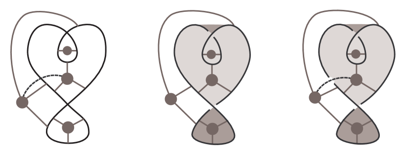
Figure 3.1.

The following is a classification of regular projections of a cycle with at most three double points. See [1, FIGURE 15].

Lemma 3-2.

Let $\varphi$ be a regular projection of a cycle $\gamma$ with ${\rm cr}(\varphi)\leq 3$. Then $\widehat{\gamma}$ is one of the ten projections as illustrated in Fig. 3.2 up to isotopy of ${\mathbb{S}}^{2}$.

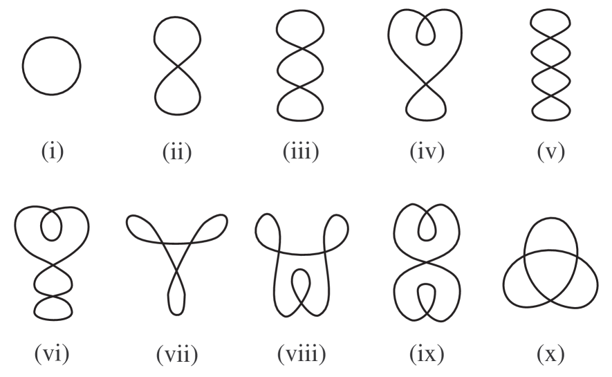
Figure 3.2.

Proof of Theorem 1-3..

Let $\gamma$ be a cycle of $G$. Let $e_{1},e_{2},\ldots,e_{m}\ (0\leq m\leq 3)$ be all different edges of $G$ which are not included in $\gamma$ such that $\widehat{\gamma}$ and $\widehat{e}_{i}$ produce double points of $\varphi$. By subdividing $G$ with some vertices of valency two if necessary, we may assume that $\widehat{\gamma}$ and $\widehat{e}_{i}$ produce exactly one double point of $\varphi$. We shall show that if $f$ does not contain a Hopf link or a trefoil knot then there exists a trivialization disk $D_{\gamma}$ for $f(\gamma)$. Then by Theorem 2-1 we have the desired conclusion. Since ${\rm cr}(\varphi)\leq 3$, $\widehat{\gamma}$ is one of the ten projections as illustrated in Fig. 3.2 up to isotopy of ${\mathbb{S}}^{2}$. Note that these regular projections are trivial except for (x). If $\widehat{\gamma}$ is any one of (iii), (iv), (v), (vi), (vii), (viii) or (ix), then the interferency of $\widehat{\gamma}$ is less than or equal to $1$ and by Lemma 3-1 there exists a trivialization disk for $f(\gamma)$. Thus, in the rest of the proof we show the claim in the case that $\widehat{\gamma}$ is (i), (ii) or (x).

Let us consider the case that $\widehat{\gamma}$ is (i) or (ii). If the interferency of $\widehat{\gamma}$ is less than or equal to $1$, then by Lemma 3-1 there exists a trivialization disk for $f(\gamma)$. So we assume that the interferency of $\widehat{\gamma}$ is $2$ or $3$. Since ${\rm cr}(\varphi)\leq 3$, we may divide our situation about the circumstances around $\widehat{\gamma}$ into the four cases (1), (2), (3) and (4) as illustrated in Fig. 3.3. We remark here that there are ambiguities for positions of the ends of $\widehat{H}_{i}$ in Fig. 3.3, but they do not have an influence on our arguments except for the case (4d) as we will say later. In the following we observe a regular diagram of a spatial embedding of $G$ which projects on (1), (2), (3) or (4).

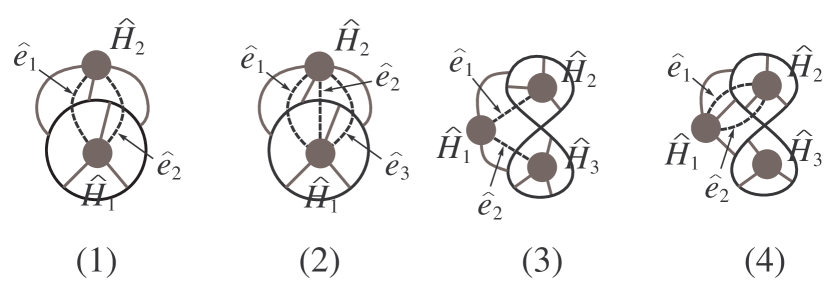
Figure 3.3.

(1) It is sufficient to consider the two cases (1a) and (1b) as illustrated in Fig. 3.4. The other cases can be shown by considering the mirror image embedding in the same way as the proof of Lemma 3-1 (after this we often adopt this argument and do not touch on it one by one). In the case (1a), it is clear that there exists a trivializing disk for $f(\gamma)$, see Fig. 3.4. Next we consider the case (1b). Since $f$ does not contain a Hopf link, we may assume that $e_{1}$ and $e_{2}$ each are incident to the different connected components of $H_{1}$ without loss of generality. Then we can see that there exists a trivializing disk for $f(\gamma)$, see Fig. 3.4.

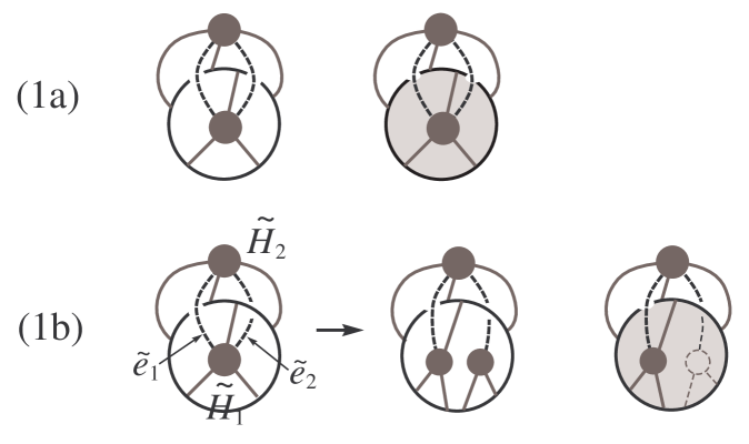
Figure 3.4.

(2) It is sufficient to consider the two cases (2a) and (2b) as illustrated in Fig. 3.5. In the case (2a), it is clear that there exists a trivializing disk for $f(\gamma)$, see Fig. 3.5. Next we consider the case (2b). Since $f$ does not contain a Hopf link, we may assume that both $e_{1}$ and $e_{2}$ are not incident to the connected component of $H_{1}$ to which $e_{3}$ is incident, or both $e_{1}$ and $e_{3}$ are not incident to the connected component of $H_{1}$ to which $e_{2}$ is incident without loss of generality. In the former case, it is clear that there exists a trivializing disk for $f(\gamma)$, see Fig. 3.5. In the latter case, we may assume that both $e_{1}$ and $e_{3}$ are incident to the same connected component of $H_{1}$. Since $f$ does not contain a Hopf link, we have that $e_{1}$ and $e_{3}$ are incident to the different connected components of $H_{2}$. If $e_{2}$ is not incident to the connected component of $H_{2}$ to which $e_{3}$ is incident, then we can see that there exists a trivializing disk for $f(\gamma)$, see Fig. 3.5. If $e_{2}$ is not incident to the connected component of $H_{2}$ to which $e_{1}$ is incident, then we also can see that there exists a trivializing disk for $f(\gamma)$, see Fig. 3.5.

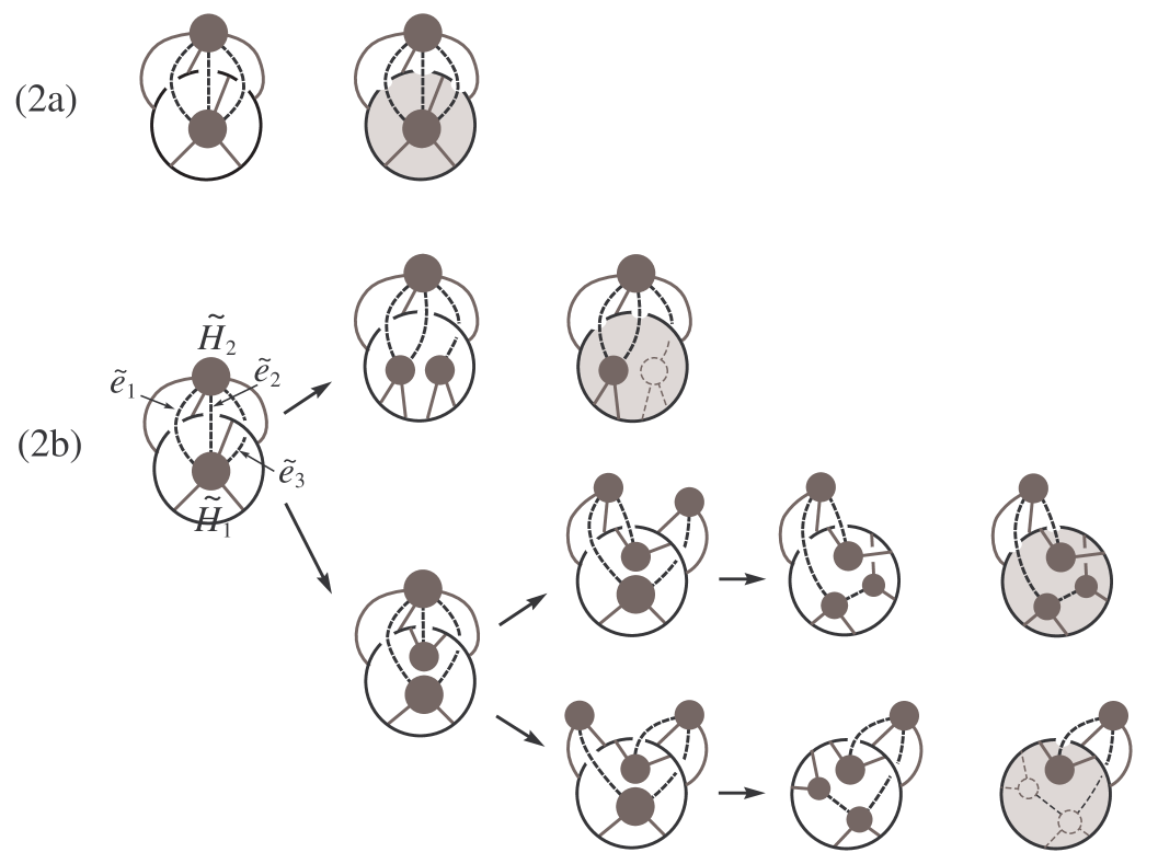
Figure 3.5.

(3) It is sufficient to consider the four cases (3a), (3b), (3c) and (3d) as illustrated in Fig. 3.6. In any cases we can see easily that there exists a trivializing disk for $f(\gamma)$, see Fig. 3.6.

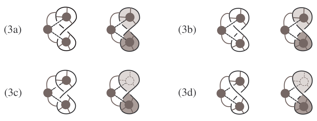
Figure 3.6.

(4) It is sufficient to consider the four cases (4a), (4b), (4c) and (4d) as illustrated in Fig. 3.7. In the cases (4a) and (4b), it is clear that there exists a trivializing disk for $f(\gamma)$, see Fig. 3.8. Next we consider the case (4c). Since $f$ does not contain a Hopf link, we have that $e_{1}$ and $e_{2}$ are incident to the different connected components of $H_{2}$, or $e_{1}$ and $e_{2}$ are incident to the different connected components of $H_{1}$. In either cases we can see that there exists a trivializing disk for $f(\gamma)$, see Fig. 3.9. Next we consider the case (4d). Since $f$ does not contain a Hopf link, we have that $e_{1}$ and $e_{2}$ are incident to the different connected components of $H_{2}$, or $e_{1}$ and $e_{2}$ are incident to the different connected components of $H_{1}$. In the former case, it is clear that there exists a trivializing disk for $f(\gamma)$, see Fig. 3.10. In the latter case, we may assume that both $e_{1}$ and $e_{2}$ are incident to the same connected component of $H_{2}$. We denote the connected component of $H_{1}$ to which $e_{i}$ is incident by $H_{1}^{(i)}\ (i=1,2)$. If there exist an end of $\widetilde{H}_{1}^{(1)}$ and an end of $\widetilde{H}_{1}^{(2)}$ each of which attaches to the boundary of $R_{3}$, then they must have a common vertex on the boundary of $R_{3}$ because $f$ does not contain a trefoil knot, see Fig. 3.11. Then we can see that there exists a trivializing disk for $f(\gamma)$, see Fig. 3.10.

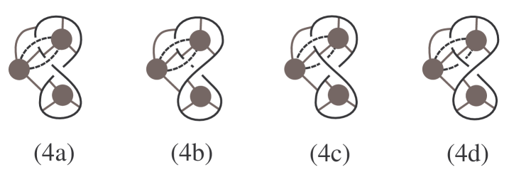
Figure 3.7.

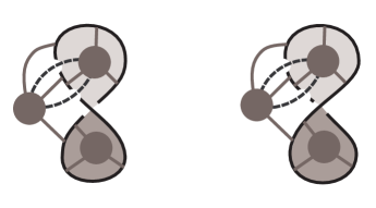
Figure 3.8.

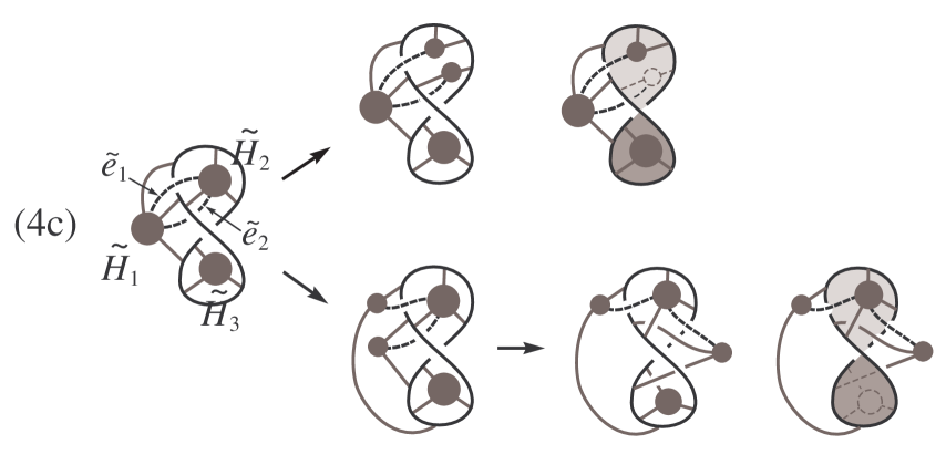
Figure 3.9.

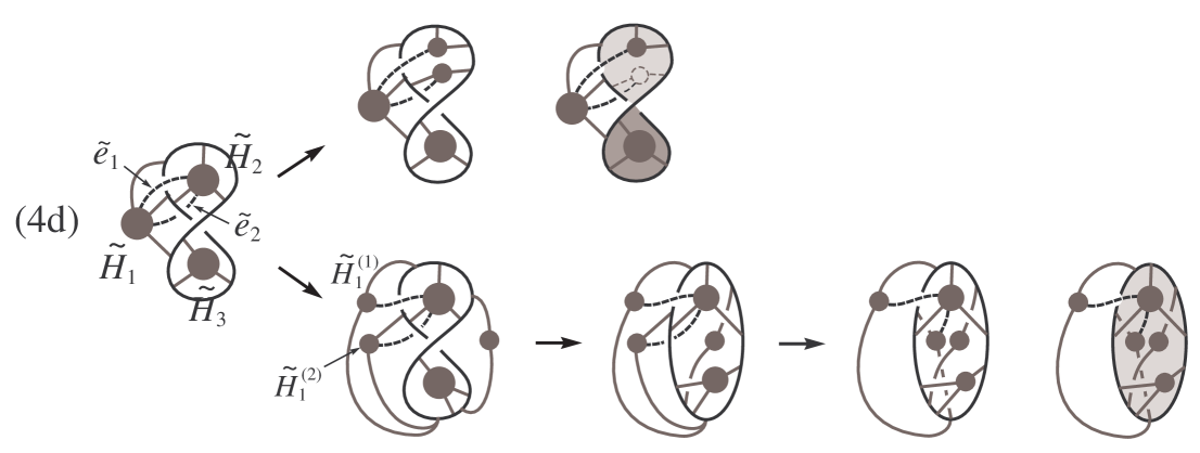
Figure 3.10.

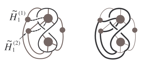
Figure 3.11.

Finally let us consider the case that $\widehat{\gamma}$ is (x). Then the interferency of $\widehat{\gamma}$ is equal to $0$ and only trivial knots or trefoil knots project on it. Since $f$ does not contain a trefoil knot, we have that $f(\gamma)$ is a trivial knot. Thus our situation about the circumstances around $\widehat{\gamma}$ can be depicted as Fig. 3.12. And we can find a trivialization disk for $f(\gamma)$, see Fig. 3.12. This completes the proof.

Figure 3.12.

∎

4. Proof of Theorem 1-1

In this section we prove Theorem 1-1. For a regular projection $\varphi$ of a graph $G$, we denote the set of all equivalence classes of spatial embeddings of $G$ which project on $\varphi$ by ${\rm SE}(\varphi)$. We say that two regular projections $\varphi$ and $\psi$ of $G$ are SE-equivalent ($\varphi\sim_{{\rm SE}}\psi$) if ${\rm SE}(\varphi)={\rm SE}(\psi)$.

Proof of Theorem 1-1..

(1) It is clear by Corollary 1-4 (1).

(2) Let $\varphi$ be a regular projection of $G$ with ${\rm cr}(\varphi)=2$. If there exists a non-trivial spatial embedding $f$ of $G$ which projects on $\varphi$, then by Corollary 1-4 (2), $f$ contains a Hopf link. Since ${\rm cr}(\varphi)=2$, there exists a pair of disjoint cycles $\gamma$ and $\gamma^{\prime}$ of $G$ such that $\widehat{\gamma}\cup\widehat{\gamma^{\prime}}$ may be described as the left-hand side of Fig. 4.1. Then it is clear that each of the double points is Type-D. Therefore we have that if $\varphi$ has a double point of Type-S or Type-A then there does not exists a non-trivial spatial embedding of $G$ which projects on $\varphi$, namely $\varphi$ is trivial.

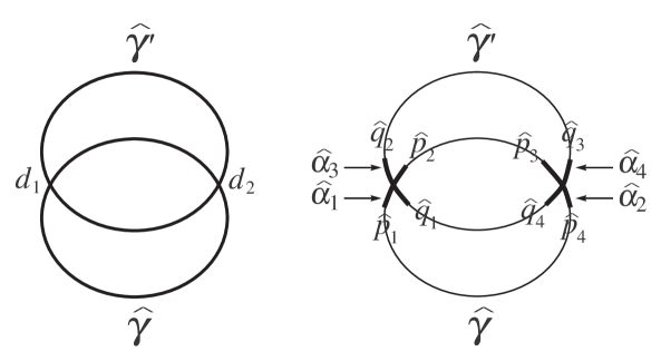
Figure 4.1.

Now we assume that $\varphi$ is knotted. Let $d_{1}$ and $d_{2}$ be exactly two double points of $\varphi$. By considering sufficiently small compact neighborhoods $N_{1}$ and $N_{2}$ of $d_{1}$ and $d_{2}$ in ${\mathbb{S}}^{2}$, respectively, we can obtain disjoint simple subarcs $\alpha_{1}$, $\alpha_{2}$, $\alpha_{3}$ and $\alpha_{4}$ of $G$ each of which does not contain any vertex of $G$, so that $\varphi^{-1}(N_{1})=\alpha_{1}\cup\alpha_{3}$, $\varphi^{-1}(N_{2})=\alpha_{2}\cup\alpha_{4}$ and $\alpha_{1}\cup\alpha_{2}\subset\gamma$, $\alpha_{3}\cup\alpha_{4}\subset\gamma^{\prime}$. We put $\partial\alpha_{1}=\left\{p_{1},p_{2}\right\}$, $\partial\alpha_{2}=\left\{p_{3},p_{4}\right\}$, $\partial\alpha_{3}=\left\{q_{1},q_{2}\right\}$ and $\partial\alpha_{4}=\left\{q_{3},q_{4}\right\}$ so that $\widehat{p_{i}}$ and $\widehat{q}_{i}\ (i=1,2,3,4)$ are in the position as illustrated in the right-hand side of Fig. 4.1. We denote two arcs $\gamma\setminus({\rm int}\alpha_{1}\cup{\rm int}\alpha_{2})$ by $\iota_{1}$ and $\iota_{2}$ so that $\partial\iota_{1}=\left\{p_{2},p_{3}\right\}$ and $\partial\iota_{2}=\left\{p_{1},p_{4}\right\}$, and two arcs $\gamma^{\prime}\setminus({\rm int}\alpha_{3}\cup{\rm int}\alpha_{4})$ by $\kappa_{1}$ and $\kappa_{2}$ so that $\partial\kappa_{1}=\left\{q_{2},q_{3}\right\}$ and $\partial\kappa_{2}=\left\{q_{1},q_{4}\right\}$. By giving over/under informations to $d_{1}$ and $d_{2}$ so that $\widetilde{\gamma}$ passes over $\widetilde{\gamma^{\prime}}$, we can obtain the spatial embedding $f$ of $G$ which projects on $\varphi$ such that $f(\gamma\cup\gamma^{\prime})$ is a trivial $2$-component link. Note that $f$ is non-trivial because $\varphi$ is knotted. Therefore by Corollary 1-4 (2), there exists a pair of disjoint cycles $\gamma^{\prime\prime}$ and $\gamma^{\prime\prime\prime}$ of $G$ such that $f(\gamma^{\prime\prime}\cup\gamma^{\prime\prime\prime})$ is a Hopf link. Since ${\rm cr}(\varphi)=2$, we may assume that $\alpha_{1}\cup\alpha_{4}\subset\gamma^{\prime\prime}$ and $\alpha_{2}\cup\alpha_{3}\subset\gamma^{\prime\prime\prime}$. Moreover, we may assume that there exists a pair of disjoint subarcs $\lambda_{1}$ and $\lambda_{2}$ of $\gamma^{\prime\prime}$ such that $\partial\lambda_{1}=\left\{p_{2},q_{3}\right\}$ and $\partial\lambda_{2}=\left\{p_{1},q_{4}\right\}$ without loss of generality. Then there exists a pair disjoint subarcs $\mu_{1}$ and $\mu_{2}$ of $\gamma^{\prime\prime\prime}$ such that $\partial\mu_{1}=\left\{p_{4},q_{2}\right\}$ and $\partial\mu_{2}=\left\{p_{3},q_{1}\right\}$. We denote the subgraph $\gamma\cup\gamma^{\prime}\cup\gamma^{\prime\prime}\cup\gamma^{\prime\prime\prime}$ of $G$ by $H$. We call the closure of a connected component of $H\setminus{\gamma\cup\gamma^{\prime}}$ in $H$ a connector. Note that a connector is a simple arc in $H$ whose boundary belongs to $\gamma\cup\gamma^{\prime}$.

Since $H$ is planar, there exists an embedding $\psi:H\to{\mathbb{S}}^{2}$. For a subspace $S$ of $H$, we denote $\psi(S)$ also by $S$ as long as no confusion occurs. Then we may assume that $\gamma\cup\gamma^{\prime}$ is positioned into ${\mathbb{S}}^{2}$ by $\psi$ as illustrated in Fig. 4.2 (1) or (2). In any of the two cases, $\gamma^{\prime}$ bounds a 2-disk $D^{\prime}$ in ${\mathbb{S}}^{2}$ whose interior does not contain $\gamma$, and $\gamma$ bounds a $2$-disk $D$ in ${\mathbb{S}}^{2}$ whose interior contains $D^{\prime}$. We denote the annulus $D\setminus{\rm int}D^{\prime}$ by $A$ and the $2$-disk ${\mathbb{S}}^{2}\setminus{\rm int}D$ by $D^{\prime\prime}$. Note that there does not exist a connector between $\iota_{1}$ and $\iota_{2}$ (resp. $\kappa_{1}$ and $\kappa_{2}$) because if such a connector exists then ${\rm cr}(\varphi)>2$. Therefore, if there exists a connector $c$ in $D^{\prime\prime}$ (resp. $D^{\prime}$) then $\partial c\subset\iota_{i}$ (resp. $\partial c\subset\kappa_{i}$) for some $i$. Then we may assume that there does not exist any connector in $D^{\prime}$ and $D^{\prime\prime}$ by making a detour through outermost connectors in $D^{\prime}$ and $D^{\prime\prime}$ if necessary.

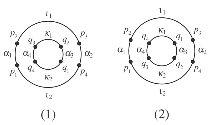
Figure 4.2.

Now let us consider the case (1) of Fig. 4.2. Since there does not exist any connector in $D^{\prime}$ and $D^{\prime\prime}$, we see that $\gamma^{\prime\prime}$ runs in $A$. Then we peel $\gamma^{\prime\prime}$ from $(\gamma\cup\gamma^{\prime})\setminus(\alpha_{1}\cup\alpha_{4})$ in $A$ by applying local deformations as illustrated in Fig. 4.3. We also peel $\gamma^{\prime\prime\prime}$ from $(\gamma\cup\gamma^{\prime})\setminus(\alpha_{2}\cup\alpha_{3})$ in the same way. By this operation, we can obtain new plane graph $H^{\prime}$ from $H$. But it is easy to see that $H^{\prime}$ contains a subspace which is homeomorphic to the complete bipartite graph on $3+3$ vertices, namely $H^{\prime}$ is non-planar, see Fig. 4.4. It is a contradiction. We can see that the case (2) of Fig. 4.2 also yields a contradiction in a similar way. Hence we have that $\varphi$ is not knotted.

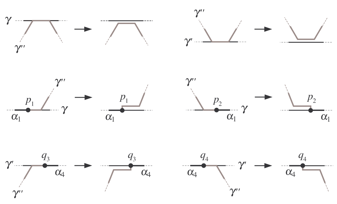
Figure 4.3.

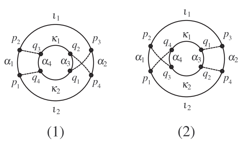
Figure 4.4.

(3) Let $\varphi$ be a regular projection of $G$ with ${\rm cr}(\varphi)=3$. If $\varphi$ has a double point of Type-S, then we may divide our situation into the three cases (a), (b) and (c) as illustrated in Fig. 4.5. In (a) and (b), $\varphi$ is SE-equivalent to a regular projection $\psi$ of $G$ with ${\rm cr}(\psi)=2$ as illustrated in Fig. 4.5. Note that $\psi$ is not knotted by Theorem 1-1 (2). Thus we have that $\varphi$ is not knotted. In (c), there exists a trivial spatial embedding of $G$ which projects on $\varphi$, see Fig. 4.5. Thus we have that $\varphi$ is not knotted.

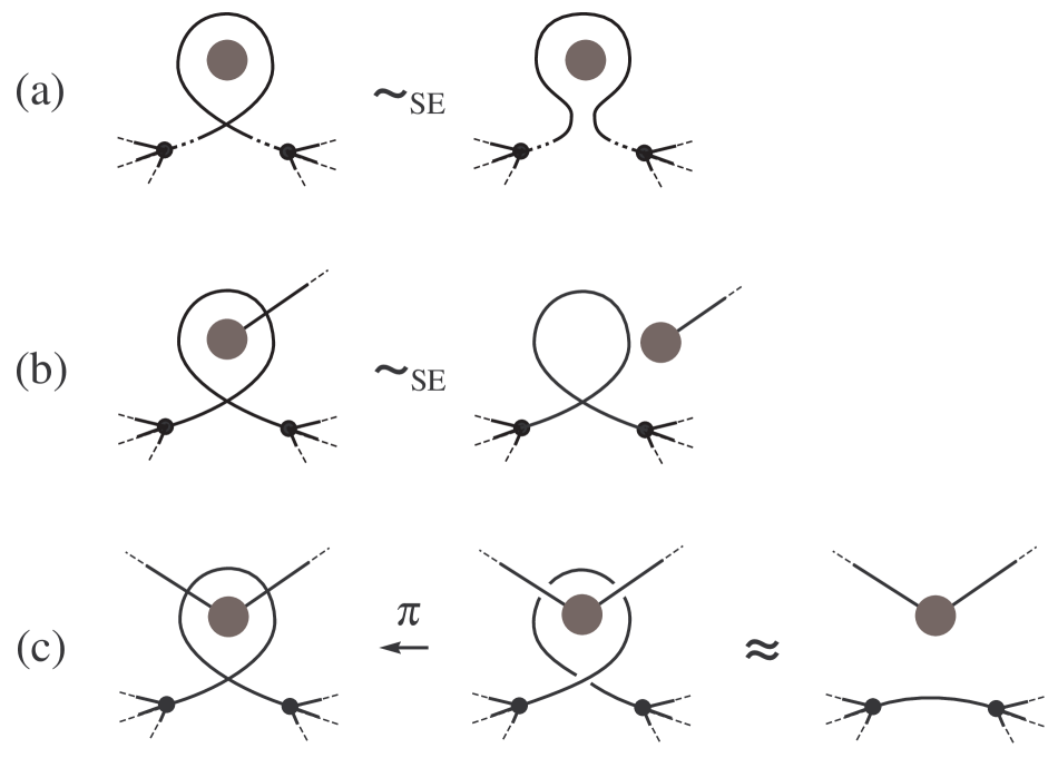
Figure 4.5.

If $\varphi$ does not have a double point of Type-S but has a double point of Type-A, then we may divide our situation into the four cases (e), (f), (g) and (h) as illustrated in Fig. 4.6. In (e) and (f), we can show that $\varphi$ is not knotted in a similar way as (a) and (b). In (g), we can also show that $\varphi$ is not knotted in a similar way as (c). In (h), let $\psi$ be a regular projection of $G$ which is obtained from $\varphi$ by smoothing the double point of Type-A as illustrated in Fig. 4.7. Since ${\rm cr}(\psi)=2$, we have that $\psi$ is not knotted by Theorem 1-1 (2). Note that any spatial embedding of $G$ which projects on $\psi$ also projects on $\varphi$, see Fig. 4.8. Thus we have that if $\varphi$ is knotted then $\psi$ is also knotted. It is a contradiction. Hence we have that $\varphi$ is not knotted.

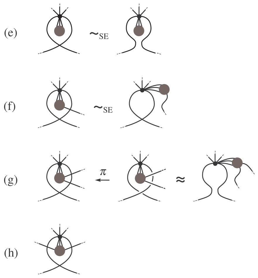
Figure 4.6.

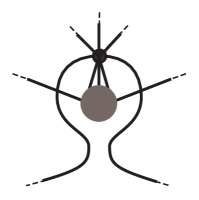
Figure 4.7.

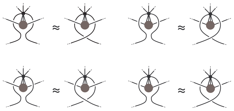
Figure 4.8.

∎

References

- [1] V. I. Arnold, Remarks on the enumeration of plane curves, Topology of real algebraic varieties and related topics, 17–32, Amer. Math. Soc. Transl. Ser. 2, 173, Amer. Math. Soc., Providence, RI, 1996.
- [2] A. Kawauchi, Almost identical imitations of -dimensional manifold pairs, Osaka J. Math. 26 (1989), 743-758.
- [3] L. Lovász, Graph minor theory, Bull. Amer. Math. Soc. (N.S.) 43 (2006), 75–86 (electonic).
- [4] R. Nikkuni, M. Ozawa, K. Taniyama and Y. Tsutsumi, Newly found forbidden graphs for trivializability, J. Knot Theory Ramifications 14 (2005), 523-538.
- [5] R. Nikkuni, Regular projections of spatial graphs, Knot Theory for Scientific Objects, Osaka City University Advanced Mathematical Institute Studies 1 111-128, Osaka Municipal Universities Press, 2007.
- [6] N. Robertson and P. Seymour, Graph minors XX. Wagner’s conjecture, J. Combin. Theory Ser. B 92 (2004), 325–357.
- [7] N. Robertson, P. Seymour and R. Thomas, Sachs’ linkless embedding conjecture, J. Combin. Theory Ser. B 64 (1995), 185-227.
- [8] M. Scharlemann and A. Thompson, Detecting unknotted graphs in -space, J. Diff. Geom. 34 (1991), 539–560.
- [9] I. Sugiura and S. Suzuki, On a class of trivializable graphs, Sci. Math. 3 (2000), 193–200.
- [10] N. Tamura, On an extension of trivializable graphs, J. Knot Theory Ramifications 13 (2004), 211–218.
- [11] K. Taniyama, Knotted projections of planar graphs, Proc. Amer. Math. Soc. 123 (1995), 3575–3579.
- [12] K. Taniyama and T. Tsukamoto, Knot-inevitable projections of planar graphs, J. Knot Theory Ramifications 5 (1996), 877-883.
- [13] Y. Q. Wu, On planarity of graphs in -manifolds, Comment. Math. Helv. 67 (1992), 635–647.
- [14] Y. Q. Wu, On minimally knotted embedding of graphs, Math. Z. 214 (1993), 653–658.