Coarse-graining stochastic biochemical networks: quasi-stationary approximation and fast simulations using a stochastic path integral technique

Abstract

We propose a universal approach for analysis and fast simulations of stiff stochastic biochemical kinetics networks, which rests on elimination of fast chemical species without a loss of information about mesoscopic, non-Poissonian fluctuations of the slow ones. Our approach, which is similar to the Born-Oppenheimer approximation in quantum mechanics, follows from the stochastic path integral representation of the full counting statistics of reaction events (also known as the cumulant generating function). In applications with a small number of chemical reactions, this approach produces analytical expressions for moments of chemical fluxes between slow variables. This allows for a low-dimensional, interpretable representation of the biochemical system, that can be used for coarse-grained numerical simulation schemes with a small computational complexity and yet high accuracy. As an example, we consider a chain of biochemical reactions, derive its coarse-grained description, and show that the Gillespie simulations of the original stiff system, the coarse-grained simulations, and the full analytical treatment are in an agreement, but the coarse-grained simulations are three orders of magnitude faster than the Gillespie analogue.

I Introduction

Single molecule biochemical experiments provide highly detailed knowledge about the mean time between successive reaction events and hence about the reaction rates. Additionally, they deliver qualitatively new information, inaccessible to bulk experiments, by measuring other reactions statistics, such as variances and autocorrelations of successive reaction times english-00 ; orrit ; gopich-03 ; english-06 ; xue-06 ; chaudhury-07 . In their turn, these quantities relate to structural properties of the reaction networks, uncovering such phenomena as internal enzyme states or multi-step nature of seemingly simple reactions, and hence starting a new chapter in the studies of the complex biochemistry that underlies cellular regulation, signaling, and metabolism.

However, the bridge between the experimental data and the network properties is not trivial. Since the class of exactly solvable biologically relevant models is limited hornos-05 ; darvey-66 ; Jayaprakash-07 , exact analytical calculations of statistical properties of reactions are impossible even for some of the simplest networks. Similarly, the variational approach sasai-03 ; lan-06 and other analytical approximations are of little help when the experimentally observed quantities depend on features that are difficult to approximate, such as the tails of the reaction events distributions. Therefore, computer simulations are often the method of choice to explore an agreement between a presumed model and the observed experimental data.

Unfortunately, even the simplest biochemical simulations often face serious problems, both conceptual and practical. First, the networks usually involve combinatorially many molecular species and elementary reaction processes: for example, a single molecular receptor with $n$ modification sites can exist in $2^{n}$ states, and an even larger number of reactions connecting them hlavacek . Second, while it is widely known that some molecules occur in the cell at very low copy numbers (e.g., a single copy of the DNA), which give rise to relatively large stochastic fluctuationslow-copy1 ; low-copy2 ; low-copy3 ; low-copy4 ; low-copy5 ; low-copy6 ; low-copy7 , it is less appreciated that the combinatorial complexity makes this true for almost all molecular species. Indeed, complex systems with a large number of molecules, like in eukaryotic cells, may have small abundances of typical microscopic species if the number of the species is combinatorially large. Third, and perhaps the most profound difficulty of the “understanding-through-simulations” approach, is that only very few of the kinetic parameters underlying the combinatorially complex, stochastic biochemical networks are experimentally observed or even observable. For example, the average rate of phosphorylation of a receptor on a particular residue can be measured, but it is hopeless to try to determine the rate for each of the individual microscopic states of the molecule determined by its modification on each of the other available sites.

While some day computers may be able to tackle the formidable problem of modeling astronomically large biochemical networks as a series of random discrete molecular reaction events (which will properly account for stochastic copy number fluctuations), and then performing sweeps through parameter spaces in search of an agreement with experiments, such powerful computers are still far away. More importantly, even if this computational ability were available, it would not help in building a comprehensible, tractable interpretation of the modeled biological processes and in identifying connections between microscopic features and macroscopic parameters of the networks.

Clearly, such an interpretation can be aided by simplifying the networks through coarse-graining, that is, by merging or eliminating certain nodes and/or reaction processes. Ideally, as in Fig. 1, one wants to substitute a whole network of elementary (that is, single-step, Poisson-distributed) biochemical reactions with a few complex reaction links connecting the species that survive the coarse-graining in a way that retains predictability of the system. Not incidentally, this would also help with each of the three major roadblocks mentioned above, by reducing the number of interacting elements, increasing the number of molecules in agglomerated hyperspecies, and combining multiple features into a much smaller number of effective, mesoscopic kinetic parameters.

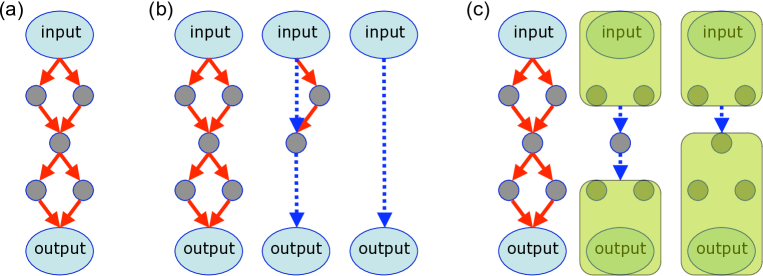
Figure 1: (a) A complex network of elementary reactions connecting the input and the output nodes. Note that the choice of these nodes usually distinguishes different coarse-graining schemes, and it is rather arbitrary. In our work, the choice is determined by the adiabatic time scale separation, as described in Methods. In principle, such networks can be coarse-grained by multiple methods. In (b) we illustrate the decimation procedure, where intermediate nodes with fast dynamics get eliminated successively, resulting in complex reactions connecting their immediate neighbors; the statistics of these complex reactions are determined by the cumulant generating functions (CGF) ${\mathcal{S}}(\chi)$, cf. Results. Other coarse-graining schemes are possible. For example, (c) nodes can be merged in hyper-nodes, again connected to each other by complex reactions. Combinations of the strategies are also allowed. Panels (b) and (c) resemble the decimation and the blocking procedures in statistical physics kadanoff , and, not coincidentally, statistical physics is the field where coarse-graining has had the biggest impact and is the most developed ma . Both the decimation and the blocking are in the spirit of the real-space renormalization group on an irregular lattice, and one can also think of momentum-space-like approaches as a complement ma .

The importance of coarse-graining in biochemistry has been understood since 1913 MM , when the first deterministic coarse-graining mechanism, now known as the Michaelis-Menten (MM) enzyme, was proposed for the following kinetic scheme:

$$E+S\xrightleftharpoons[k_{-1}{[C]}]{k_{1}[E][S]}C\xrightarrow{k_{2}[C]}E+P.$$ (1)

Here $k_{1}$, $k_{2}$, and $k_{-1}$ are kinetic rates, $S$, $P$, $E$, and $C$ denote the substrate, the product, the enzyme, and the enzyme-substrate complex molecules, respectively, and $[\dots]$ represent the abundances. The enzyme catalyzes the $S\to P$ transformation by merging with $S$ to create an unstable complex $C$, which then dissociates either back into $E+S$ or forward into $E+P$, leaving $E$ unmodified. If $[S]\gg[E]$, then the enzyme cycles many times before $[S]$ and $[P]$ change appreciably. This allows to simplify the enzyme-mediated dynamics by assuming that the enzymes equilibrate quickly at the current substrate concentration, resulting in a coarse-grained, complex reaction with decimated enzyme species:

$$S\xrightarrow{v}P,\quad v=\frac{k_{2}[S][E]}{[S]+(k_{2}+k_{-1})/k_{1}}.$$ (2)

However, this simple reduction is insufficient when stochastic effects are important: each complex MM reaction consists of multiple elementary steps, thus the statistics of the number of MM reactions per unit time, in general, is non-Poissonian. While some relatively successful attempts have been undertaken to extend simple deterministic coarse-graining to the stochastic domain arkin-1 ; arkin-2 ; arkin-3 ; gopich-06 ; sinitsyn-07epl , a general set of tools for coarse-graining large biochemical networks has not been found yet.

In this article, we propose a method for a systematic rigorous coarse-graining of stochastic biochemical networks, which can be viewed as a step towards creation of comprehensive coarse-grained analysis tools. We start by noting that, in addition to the conceptual problems mentioned above, a technical difficulty stands in the way of stochastic simulations methods in systems biology: molecular species and reactions have very different dynamical time scales, which makes biochemical networks stiff and difficult to simulate. Here we propose to use this property of separation of time scales to our advantage.

The idea is not new, and multiple related approaches have been proposed in the literature, differing from each other mainly in the definition of fast and slow variables. A common practice is to use reaction rates to identify fast and slow reactions arkin-1 ; arkin-2 ; arkin-3 . However, if two species of very different typical abundances are coupled by one reaction, then a relatively small change in the concentration of the high abundance species can have a dramatic effect on that of the low abundance one. This notion of species-based rather than reaction-based adiabaticity has been used in the original MM derivation, and it is also at the heart of our arguments.

Our method builds upon the stochastic path integral technique from mesoscopic physics pilgram-03 ; pilgram-04 ; elgart-04 ; sinitsyn-07prl , providing three major improvements that make the approach more applicable to biological networks. First, we extend the method, initially developed for large copy number species, to deal with simple discrete degrees of freedom, such as a single MM enzyme or a single gene. Second, we explain how to apply the technique to a network of multiple reactions, thereby reducing the entire network to a single complex reaction step. Finally, we show how the procedure can be turned into an efficient algorithm for simulations of coarse-grained networks, while preserving important statistical characteristics of the original dynamics. The algorithm is akin to the Langevin zinn-justin or $\tau$-leaping tau-leapin1 ; tau-leapin2 schemes, widely used in biochemical simulations, but it allows to simulate an entire complex reaction in a single step. We believe that this development of a fast, yet precise simulation algorithm is the most important practical contribution of this manuscript.

For pedagogical reasons, we develop the method using a model system that is simple enough for a detailed analysis, yet is complex enough to support our goals. A generalization to more complex systems is suggested in the Discussion.

I.1 The model

Consider the system in Fig. 2: an enzyme is attached to a membrane in a cell. $S_{\rm B}$ substrate molecules are distributed over the bulk cell volume. Each molecule can either be adsorbed by the membrane, forming the species $S_{\rm M}$, or dissociate from it. Enzyme-substrate interactions are only possible in the adsorbed state. One can easily recognize this as an extremely simplified model of receptor mediated signaling, such as in vision GFP ; detwiler-00 , or immune signaling.

As usual, the enzyme-substrate complex $C$ can split either into $E+S$ or into $E+P$. Let’s suppose that the latter reaction is observable; for example, a GFP-tagged enzyme sparks each time a product molecule is created english-06 . We further suppose the reaction $C\to E+P$ is not reversible (that is, the product leaves the membrane or the reaction requires energy and is far from equilibrium).

The full set of elementary reactions is

1. adsorption of the bulk substrate onto the membrane, $S_{\rm B}\rightarrow S_{\rm M}$, with rate $q_{0}S_{\rm B}$;

2. reemission of the substrate back into the bulk, $S_{\rm M}\rightarrow S_{\rm B}$, with rate $qS_{\rm M}$;

3. Michaelis-Menten conversion of $S_{\rm M}$ into $P$, consisting of

   1. substrate-enzyme complex formation, $S_{M}+E\rightarrow C$, with rate $k_{1}S_{\rm M}$;

   2. complex backward decay, $C\rightarrow S_{\rm M}+E$, with rate $k_{-1}$;

   3. product emission $C\rightarrow E+P$, with rate $k_{2}$.

Note that here and in the rest of the article, we drop the $[\dots]$ notation for denoting abundances and don’t make a distinction between a species name and the number of its molecules.

In this setup, only emission of the product is directly observable. Our goal is to coarse-grain the above system of five reaction processes into a single complex reaction $S_{\rm B}\to P$, as in Fig. 3(c). That is, we want to eliminate all intermediate species and reaction processes, while preserving their effects on the statistical properties of the complex reaction $S_{\rm B}\to P$ on time scales appropriate for its dynamics.

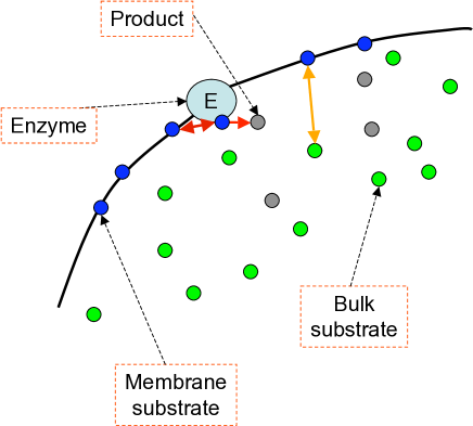
Figure 2: A single enzyme on a membrane, interacting with substrate molecules. Green, blue, and grey circles are bulk substrate, membrane substrate, and product molecules, respectively. Arrows represent possible reactions: (1,2) adsorption and dissociation of $S$ by/from the membrane (orange); (3) multi-step MM conversion $S\to P$ (red).

This set of reactions has another interpretation. Consider an MM enzyme in the bulk together with the substrate. When the substrate concentration is small, only few of its molecules are sufficiently close to the enzyme to interact with it. In this context, one can approximate the full reaction-diffusion setup by a system having an inner (reactive) and an outer (non-reactive) regions surrounding the enzyme. Diffusion takes substrate molecules between the regions with (almost) Poisson statistics of transitions, with the rate parameters depending on the volume of the regions and the diffusion coefficient. The particles in the inner region can interact with the MM enzyme, completing the mapping between the reaction-diffusion system and the multi-state well-mixed kinetic process described above.

II Results

There are three distinct effective time scales in the system in Fig. 2. One is the time scale $\tau_{\rm B}$ of the variation of the bulk substrate abundance. We assume that $S_{\rm B}$ is much larger than $S_{\rm M}$. Therefore, this time scale is the slowest, and we will be interested in studying the response of the system to the bulk substrate abundance $S_{\rm B}$ on this scale. A faster time scale is given by the dynamics of the molecules on the membrane, $\tau_{\rm M}$. Finally, at the other extreme, the fastest time scale, $\tau_{\rm E}$, is set by single reaction events, that is, the characteristic time between two successive product releases by the enzyme. Overall, $\tau_{\rm E}\ll\tau_{\rm M}\ll\tau_{\rm B}$.

We emphasize again that all species in the problem are connected by reactions that happen with approximately the same rates, and the separation of the time scales is a direct result of the particle abundances, rather than the conversion speeds: it takes only a few reaction events to change a low-abundance species drastically, and a lot longer to do the same to a high-abundance one. This is the main reason why we believe that this illustrative model will shed light on coarse-graining of a wide class of networks.

The hierarchy of times allows us to coarse-grain the system in two steps, as in Fig. 3. First, we remove the variable with the fastest dynamics, that is, the binary occupancy substrate-enzyme complex $C$. This replaces the three reactions of the MM mechanism with a single reaction $S_{\rm M}\to P$ (Fig. 3(b)). Additionally, we represent the other reactions in the system in a form more suitable for the subsequent developments. In the second step, we eliminate the membrane-bound substrate variable, which evolves on the scale $\tau_{\rm M}$. This results in the characterization of the average flux and its fluctuations for $S_{\rm B}\to P$ transformation, treating $S_{\rm B}$ as a time-dependent input parameter, cf. Fig. 3(c).

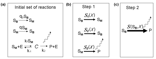
Figure 3: Coarse-graining of the model. In (a) we show the original set of reactions describing the system in Fig. 2. Panel (b) represents the set of reactions after the first coarse-graining step. Note that here the three stages of the MM enzyme have been replaced by a single complex reaction. Further, all the remaining (simple or complex) reactions are now represented by their slowly varying CGFs. Panel (c) shows the final reaction that describes the system at time scales much larger than the characteristic time of evolution of $S_{\rm M}$, the number of the substrate molecules on the membrane. The wavy line corresponds to a spark of the tracer molecule english-06 , which counts the number of $S_{\rm B}\to P$ transformations.

II.1 Preliminaries

Let $\delta Q_{\mu}$ stand for the number of reaction events for the reaction type $\mu$ (in our example, $\mu=1,2,3$ corresponds to adsorption, detachment, and the whole MM reaction, respectively). Then $P(\delta Q_{\mu}|T)$ is the probability distribution of the number of events of type $\mu$ during a temporal window of length $T$. Instead of considering these distributions directly, our derivation for the coarse-graining relies the corresponding moment generation functions (MGFs):

$${\mathcal{Z}}_{\mu}(\chi,T)=e^{{\mathcal{S}}_{\mu}(\chi,T)}=\sum_{\delta Q_{\mu}=0}^{\infty}P(\delta Q_{\mu}|T)e^{i\delta Q_{\mu}\chi}.$$ (3)

where ${\mathcal{S}}_{\mu}(\chi)$ is the cumulant generating function (CGF). The moments and the (complex) cumulants of the distribution $P(\delta Q_{\mu}|T)$ can be calculated by differentiating the MGF and the CGF, respectively

$$m_{\mu,a} = (-i)^{a}\left.\frac{\partial^{a}}{\partial\chi^{a}}\right|_{\chi=0}{\mathcal{Z}}_{\mu}(\chi,T)$$ (4)

$$c_{\mu,a} = (-i)^{a}\left.\frac{\partial^{a}}{\partial\chi^{a}}\right|_{\chi=0}{\mathcal{S}}_{\mu}(\chi,T),$$ (5)

where $a$ stands for the order of the moment (cumulant). In particular, the average flux for the reaction $\mu$ is $c_{\mu,1}=m_{\mu,1}$, and the corresponding variance is $\sigma^{2}_{\mu}=c_{\mu,2}=m_{\mu,2}-m_{\mu,1}^{2}$.

II.2 Step 1: The generating function representation

This step can be viewed as a generalization of the standard $\tau$-leaping approximation tau-leapin1 ; tau-leapin2 , which prescribes to simulate elementary, exponentially distributed reaction events, for example attachment/detachment reactions in Fig. 3(a), by choosing a time step such that the number of the reactions in it is much larger than unity, yet the reaction rates (determined by the dynamics of the slower variables in the problem) can be considered stationary. In a $\tau$-leaping scheme, one then approximates the distribution of the number of reaction events by a Poisson distribution.

Unfortunately, not all biochemical processes can be treated in such a simple manner. For example, due to the single-copy nature of the MM enzyme in our system, Fig. 3(a), the instantaneous rate of the product creation is a fast varying function of time, switching between zero and $k_{2}$ every time binding/unbinding events happen. Therefore, one cannot use $\tau$-leaping or Langevin schemes zinn-justin ; tau-leapin1 ; tau-leapin2 , or treat the product creation as a homogeneous Poisson process. We would like to avoid being forced into the Gillespie gillespie or the StochSim StochSim analysis schemes. Since either of these schemes is based on Monte-Carlo simulations of every individual reaction event, the estimation of parameters of interest may become excessively slow in large systems.

As an alternative, we will identify good approximations for the distribution of the number of reactions in a fixed time interval, which is no longer a Poisson distribution, by characterizing its CGF (see Methods: Moment generating functions for elementary chemical reactions). To this end, we propose to eliminate the binary substrate-enzyme complex variable and reduce the MM reaction triplet to a single reaction, whose dynamics can be considered stationary over times much longer than a single reaction event. This completes Step 1 of the coarse-graining in which each reaction, or a small complex of reactions, is subsumed by a CGF ${\mathcal{S}}_{\mu}$ of the distribution of the number of events, which can be considered stationary for extended times. Importantly, in this Step, we removed the only species in the problem that exists, at most, in a single copy and hence is stiff. This dramatically simplifies simulations and analysis of the system.

The details of this are given in Methods: Coarse-graining the Michaelis-Menten reaction. In particular, in Eq. (34) we derive ${\mathcal{S}}_{3}$, the CGF for the entire complex Michaelis-Menten reaction, eliminating the intermediate substrate-enzyme complex $C$. The expression is valid over times much larger than $\tau_{\rm E}$, but smaller than $\tau_{\rm M}$, so that many enzyme turnovers happen, but the effect on the abundance of the membrane-bound substrate is still relatively small.

In the MM mechanism, the backward reaction is often a simple dissociation, whereas the forward one requires crossing an energy barrier and is exponentially suppressed. As a result, one often has $k_{-1}\gg k_{2}$, which can make the MM reaction doubly stiff, requiring multiple binding events (and with them the instantaneous rate changes) for each released product. Therefore, replacing the entire MM mechanism with a single complex reaction step has a dramatic effect on analysis of the reaction, and specifically on the simulation efficiency, which can now be performed using the Langevin-like quasi-stationary approximation.

To illustrate this, using Eq. (34), we write the first few cumulants of the number of MM product releases per time $\delta t$:

$$\mu_{3} = \frac{k_{1}k_{2}S_{\rm M}}{K}\,\delta t,\quad K=k_{1}S_{\rm M}+k_{2}+k_{-1},$$ (6)

$$\sigma^{2}_{3} = \mu_{3}F,\quad F=\left(1-\frac{2k_{1}k_{2}S_{\rm M}}{K^{2}}\right),$$ (7)

$$c_{3,3} = \mu_{3}\left(1-\frac{6Q(K-2Q)}{K^{2}}\right),\quad Q=\mu_{3}/\delta t,$$ (8)

$$c_{3,4} = \mu_{3}\left(1-\frac{2Q(7K^{2}-36KQ+60Q^{2}}{K^{3}}\right).$$ (9)

The coefficient $F$ in the expression for $\sigma^{2}_{3}$ is called the Fano factor (see below). To the extent that $\sigma^{2}_{3}\neq\mu_{3}$, this complex reaction is non-Poisson, as illustrated in Fig. 4.

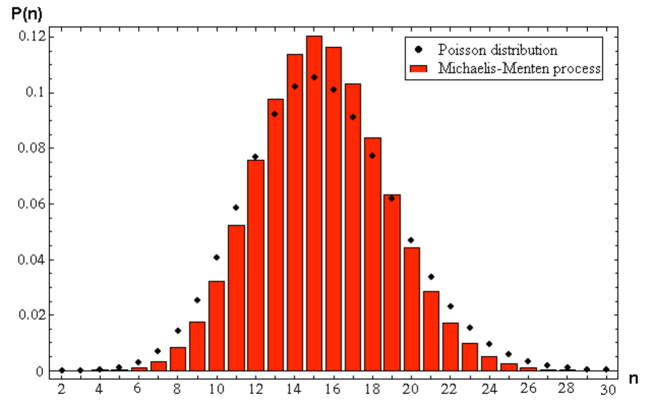
Figure 4: Distribution of the number of Michaelis-Menten reactions over a time $\delta t=35$ with $S_{\rm M}=140$, $k_{1}=0.01$, $k_{-1}=1$, and $k_{2}=1$ vs. the Poisson distribution with the same average number of reactions. The distribution for the MM process is obtained using the Gram-Charlier expansion with the four known cumulants, see Methods.

Knowing cumulants of the reaction events distribution allows for a simple numerical simulation procedure

$$\delta Q_{3}(t) = \eta_{3}(t,\delta t),$$ (10)

$$S_{\rm M}(t+\delta t) = S_{\rm M}(t)-\delta Q_{3}(t)+J(t)\delta t,$$ (11)

$$P(t+\delta t) = P(t)+\delta Q_{3}(t),$$ (12)

where $\eta_{3}(t)$ is a random variable with the cumulants given by Eqs. (6-9), and $J(t)$ represents currents exogenous to the MM reaction, such as changes in $S_{\rm M}$ due to membrane binding/unbinding. Notice that, in this step, we are now treating the single-particle-mediated reaction in a quasi-stationary, $\tau$-leaping or Langevin-like way by drawing a (random) number of complex reaction events over a time $\delta t$ directly, assuming that all parameters defining the reaction are constants over this time. The price for the coarse graining is that instead of characterizing any reaction by a single rate that defines a Poisson distribution of reaction events, one is forced to use a distribution with the prescribed sequence of moments for the Monte-Carlo simulations.

In principle, generation of such random variables is a difficult and an ill-posed task since the moments do not define the distribution uniquely, and two distributions with matched moments can be arbitrarily different from each other. Additionally, once we allow for a nonzero third or fourth cumulant, the remaining higher order cumulants cannot be zero anymorelax , and the generated random variable will depend on the assumptions made about them. Fortunately, in our case, the situation is simplified because all $c_{3,k}\sim\delta t$. Thus the $k$’th cumulant will have a progressively smaller effect, $\sim(\delta t)^{1/k}$, on a number drawn from the distribution, and our random variables are almost Gaussian. Then the Gram-Charlier series expansion edgeworth aided either by the importance or rejection sampling imp-sampl reduces the simulation scheme, Eqs. (10-12), to a simple Langevin simulation with a Gaussian noise and a small penalty, as described in Methods: Simulations with near-Gaussian distributions; see also Fig. 8 in Methods for illustration of the precision provided by these tools.

II.3 Step 2: Coarse-graining membrane reactions

For Step 2 of our coarse-graining approach, we are given the CGFs $S_{\mu}$, $\mu=1,2,3$, of the slowly varying reactions. Using the stochastic path integral technique, we then express the CGF of the entire coarse-grained reaction $S_{\rm B}\to P$ in Fig. 3(c) in terms of the component CGFs, and then simplify the expression to account for the time scale separation between the dynamics of $S_{\rm B}$ and $S_{\rm M}$. This is presented in detail in Methods: Coarse-graining all membrane reactions, cf. Eq. (48). This formally completes the coarse-graining. That is, we find the CGF of the $S_{\rm B}\to P$ particle flux for times $T\lesssim\tau_{\rm B}$, much longer than $\tau_{\rm E}$ and $\tau_{\rm M}$, the other time scales in the problem.

The resulting CGF depends on microscopic reaction rates, which can depend on slow parameters, such as $S_{\rm B}$. The full expression for CGF is cumbersome and non-illuminating. Fortunately, we only want to calculate the first few cumulants of the reaction events distribution, and these are obtained by differentiation the CGF as in Eq. (5). This gives

$$c_{1} = T\frac{1}{2k_{1}}\bigg{[}k_{1}(k_{0}+k_{2})+q(k_{2}+k_{-1})$$ (13)

$$-\sqrt{k_{1}^{2}(k_{0}-k_{2})^{2}+2k_{1}q(k_{0}+k_{2})(k_{2}+k_{-1})+q^{2}(k_{2}+k_{-1})^{2}}\bigg{]},$$

$$c_{2} = Fc_{1},$$ (14)

$$F=1-\frac{q(2k_{1}k_{0}k_{2}+k_{1}(k_{0}+k_{2})k_{-1}+qk_{-1}(k_{2}+k_{-1}))}{k_{1}^{2}(k_{0}-k_{2})^{2}+2k_{1}q(k_{0}+k_{2})(k_{2}+k_{-1})+q^{2}(k_{2}+k_{-1})^{2}}+$$ (15)

$$\quad\quad\quad\quad+\frac{qk_{-1}}{\sqrt{k_{1}^{2}(k_{0}-k_{2})^{2}+2k_{1}q(k_{0}+k_{2})(k_{2}+k_{-1})+q^{2}(k_{2}+k_{-1})^{2}}}.$$

$$c_{3} = -T\frac{\kappa}{\rho(-\kappa k_{1}+\rho^{2})^{5}}\left\{\kappa^{5}k_{1}^{5}-\rho^{10}+\kappa\rho^{7}\left[5k_{1}^{2}k_{2}+q\left(11k_{1}+6q\right)s\right]\right.$$ (16)

$$-\kappa^{2}k_{0}^{2}k_{1}^{4}\rho^{2}\left[5k_{1}^{2}k_{2}^{2}+6k_{2}\left(k_{1}-2q\right)qs+24q^{2}s^{2}\right]$$

$$+2\kappa^{2}k_{0}k_{1}^{2}\rho^{3}\left[5k_{1}^{3}k_{2}^{2}+k_{2}q\left(14k_{1}^{2}-9k_{1}q-6q^{2}\right)s+6q^{2}\left(5k_{1}+3q\right)s^{2}\right]$$

$$\left.-2\kappa k_{0}k_{1}\rho^{4}\left[5k_{1}^{4}k_{2}^{3}+19k_{1}^{3}k_{2}^{2}qs+9k_{1}^{2}k_{2}q^{2}s^{2}+6k_{2}q^{4}s^{2}+3k_{1}q^{3}s\left(-2k_{2}^{2}+8k_{2}s+s^{2}\right)\right]\right\},$$

where $s=k_{1}\langle S_{\rm M}\rangle+k_{2}+k_{-1}$, $\langle S_{\rm M}\rangle=\frac{1}{2k_{1}q}\Big{\{}k_{0}k_{1}-k_{1}k_{2}-k_{2}q-k_{-1}q+\big{[}4k_{1}k_{0}q(k_{2}+k_{-1})+(k_{1}k_{2}-k_{1}k_{0}+k_{2}q+k_{-1}q)^{2}\big{]}^{1/2}\Big{\}}$ is the average number of membrane-bound substrates, $k_{0}=q_{0}S_{\rm B}$, $\kappa=k_{0}k_{1}k_{2}$, $\rho=k_{1}k_{2}+qs$, and, finally, $T$ is the time step over which $S_{\rm B}$ changes by a relatively small amount, but many membrane reactions happen.

By analogy to the MM reaction, Eqs. (10-12), the results from Step 2 allow for simulations of the whole reaction scheme in one Langevin-like step:

$$\delta Q(t) = \eta(t,T),$$ (17)

$$S_{\rm B}(t+T) = S_{\rm B}(t)-\delta Q(t)+J(t)T,$$ (18)

$$P(t+T) = P(t)+\delta Q(t),$$ (19)

where $\eta$ is a random variable with the cumulants as in Eqs. (13-16), to be generated as in Methods: Simulations with near-Gaussian distributions, and $J(t)$ is an external current, such as production or decay of the bulk substrate in other cellular processes.

II.4 Fano factor in a single molecule experiment

In analyses of single molecule experiments, one often calculates the ratio of the variance of the reaction events distribution to its mean, called the Fano factor english-06 ; fano-ref1 :

$$F=\frac{c_{2}}{c_{1}}.$$ (20)

The Fano factor is zero for deterministic systems and one for a totally random process described by a Poisson number of reactions. As a result, the Fano factor provides a natural quantification of the importance of the stochastic effects in the studied process. In vivo, it can be measured, for example, by tagging the enzyme with a fluorescent label that emits light every time a product molecule is released english-06 .

Traditionally, to compare experimental data to a mathematical model, one would simulate the model using the Gillespie kinetic Monte Carlo algorithm gillespie , which is a slow and laborious process that takes a long time to converge to the necessary accuracy (see below). In contrast, our coarse-graining approximations yields an analytic expression for the Fano factor of the $S_{\rm B}\to P$ transformation via Eq. (15). This illustrates a first practical utility of our coarse-graining approach. In Fig. 5, we compare this analytical expression, derived under the aforementioned quasi-stationary assumption, with stochastic simulations for the full set of elementary reactions in Fig. 3(a). The results are in an excellent agreement, illustrating the power of the analytical approach.

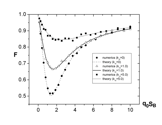
Figure 5: Comparison of the analytically calculated Fano factor for the $S_{\rm B}\to P$ reaction, Eq. (15), to direct Monte Carlo simulations with the Gillespie algorithm gillespie . Here we use $q=0.02$, $k_{1}=0.05$, $k_{2}=1$, evolution time $T=10000$ (in arbitrary units). Each numerical data point was obtained by averaging 10000 simulation runs.

Note that the Fano factor is generally different from unity, indicating a non-Poissonian behavior of the complex reaction. The backwards decay of $C$, parameterized by $k_{-1}$, adds extra randomization and thus larger values of $k_{-1}$ increases the Fano factor $F$. At another extreme, when $k_{-1}=0$, the Fano factor may be as small as 1/2, indicating that then the entire $S_{\rm B}\to P$ chain can be described by the sum of two Poisson events with similar rates, which halves the Fano factor. Finally, when $q=0$, i.e., the substrates are removed from the membrane only via conversion to products, the Fano factor $F$ is one. This is because here the only stochasticity in the problem arises from Poisson membrane binding: on long time-scales, all bound substrates will eventually get converted to the outgoing flux.

II.5 Computational complexity of coarse-grained simulations

As we alluded to before, in addition to analytical results, such as the expression for the Fano factor, we expect the coarse-graining approach to be particularly useful for stochastic simulations in systems biology. This is due to an essential speedup provided by the method over traditional simulation techniques, such as, in particular, the Gillespie algorithm gillespie , to which most other approaches are compared too.

Indeed, for the model analyzed in this work, the computational complexity of a single Gillespie simulation run is $O\left(M\frac{T}{\tau_{\rm E}}\right)$, where $M=5$ is the number of reactions in the system, and $T$ is the duration of the simulated dynamics. In contrast, the complexity of the coarse-grained approach scales as $O\left(M^{0}\left(\frac{T}{\tau_{\rm E}}\right)^{0}\right)$ since we have removed the internal species and simulate the dynamics in steps of $\sim T$, instead of steps $\sim\tau_{E}$. However, since the coarse-grained approach requires generation of complicated random numbers, the actual reduction in the complexity is unclear. More importantly, the Gillespie algorithm is (statistically) exact, while our analysis relies on quasi-stationary assumptions. Therefore, to gauge the practical utility of our approach in reducing the simulation time while retaining a high accuracy, we benchmark it against the Gillespie algorithm. We do this for a single MM enzyme first, and then progress to the full five reaction model of the enzyme on a membrane. Details of the computer system used for the benchmarking can be found in Methods: Simulations details.

The Michaelis-Menten model: We consider a MM enzyme with $S_{\rm M}=140={\rm const}$, $k_{1}=0.01$, $k_{-1}=2.0$, $k_{2}=1.0$. We analyze the number of product molecules produced by this enzyme over time $\delta t=35$, with the enzyme initially in the (stochastic) steady state. To strain both methods, we require a very high simulation accuracy, namely convergence of the fourth moment of the product flux distribution to two significant digits. For both methods, this means over 10 millions realizations of the same evolution.

Cumulants	Gillespie	Coarse-grained	Analytical prediction
$c_{1}$	11.24 $\pm$ 0.01	11.14 $\pm$ 0.01	11.14
$c_{2}/c_{1}$	0.843 $\pm$ 0.001	0.855 $\pm$ 0.001	0.855
$c_{3}/c_{1}$	0.613 $\pm$ 0.004	0.628 $\pm$ 0.004	0.628
$c_{4}/c_{1}$	0.32 $\pm$ 0.02	0.32 $\pm$ 0.02	0.319
time	8 min 45 s	12 s	N/A

Table 1: Comparison of the Gillespie and the coarse-grained simulation algorithms. The numbers are reported for 12 million realizations of the same evolution for each of the methods. To highlight deviations from the Poisson and the Gaussian statistics, we provide ratios of the higher order cumulants to the mean of the product flux distribution. In the last column, we report analytical predictions, Eqs. (6-9), obtained from the quasi-steady state approximation to the CGF.

In Tbl. 1 we report the results of our simulations. We see that the analytical coarse-grained results differ from the exact Gillespie simulations by, at most, two per cent, which is an expected deviation given the quality of the steady-state approximation. Further, the Langevin-like coarse-grained simulations, which accounted for the first four cumulants of the reaction events distribution, as in Methods: Simulations with near-Gaussian distributions, produce results nearly indistinguishable from the analytical expressions, and, again, at most two per cent different from the Gillespie runs. Yet coarse-grained simulations require only 1/40th the time of their Gillespie analogue since the time step is large, $\delta t=35$.

It is hard to imagine a practical situation in modern molecular biology where the kinetic parameters are known well enough so that the few per cent discrepancy between the full and the coarse-grained simulations matters. Yet the reduction of the simulation time by the factor of over 40 is certainly a tangible improvement.

The Michaelis-Menten enzyme on a membrane: As the next step, we compare the algorithms when the MM enzyme is embedded in the membrane, and random substrate-membrane binding/unbinding events happen in addition to the MM product production [i.e., the coarse-graining is stopped after Step 1, Fig. 3(b)]. We use parameters $k_{1}=0.02$, $k_{-1}=2$, $k_{2}=1$, $q=0.01$, and $q_{0}S_{\rm B}=1.5$. Total time of the evolution is $T=1000$, and the initial number of the substrates on the membrane is $S_{\rm M}(t=0)=120$. Finally, the relaxation time of a typical fluctuation of $S_{\rm M}$ can be estimated as $\tau_{\rm M}\sim 1/[q+(\partial k_{\rm MM}/\partial S_{\rm M})]\sim 80$, where $k_{\rm MM}$ is the rate of the Michaelis-Menten reaction for a given $S_{\rm M}$.

On time scales of $\sim\delta t$, the binding/unbinding events are Poisson distributed and can be simulated by the standard $\tau$-leaping techniques tau-leapin1 . However, for consistency, we simulate them similarly to the MM-reaction, approximating the Poisson distribution by its Gram-Charlier-series.

Since, in this setup, many events are futile membrane bindings-unbinding, the Gillespie simulations become quite time consuming, and we only achieve convergence of the first three cumulants in a reasonable time, with the third cumulant known to about two significant digits. For the coarse-grained runs, we choose the time step $\delta t=20\ll\tau_{\rm M}$, and we model all three coarse-grained reactions preserving their first three cumulants only. In this example, our coarse-grained approach speeds simulations 60-fold, yet it still provides accurate results for the first three cumulants of the distribution, see Tbl. 2.

cumulant	Gillespie	Coarse-grained (step1)	Coarse-grained (step 2)	Analytical prediction
$c_{1}$	418.7 $\pm$ 0.1	420.0 $\pm$ 0.1	418.9 $\pm$ 0.1	418.9
$c_{2}/c_{1}$	0.771 $\pm$ 0.001	0.764 $\pm$ 0.002	0.768 $\pm$ 0.001	0.767
$c_{3}/c_{1}$	0.50 $\pm$ 0.03	0.46 $\pm$ 0.08	0.48 $\pm$ 0.03	0.472
time	1h 14min	1min 17s	1s	N/A

Table 2: Comparison of cumulants of the product flux for the full system membrane calculated using the Gillespie simulations, the coarse-grained simulations (with $\delta t=20$), the fully coarse-grained simulations ($\delta t=1000$), and the analytical predictions. The data were averaged over $10^{6}$ realizations, sufficient to estimate the third cumulant to two significant digits.

The full $S_{\rm B}\to P$ conversion: Finally, we perform similar benchmarking for the Gillespie simulations and the coarse-grained simulations of the fully coarse-grained system, represented as a single complex reaction $S_{\rm B}\to P$. The third column in Tbl. 2 presents the data for this coarse-graining level. Note that representing all five reactions as a single one results in a dramatic speedup of about 4000. This number relates to the ratio of the slow and the fast time scales in the problem, but also to the fact that futile bindings-unbindings are leaped over in the coarse-grained scheme.

II.6 Generalizations to a network of reactions

As discussed in detail in the original literature (the best pedagogical exposition is in Ref. pilgram-04, ), in the stochastic path integral formalism, a network of $M$ reactions with $N$ chemical species (cf. Fig. 6) is generally described by $2MN$ ordinary differential equations specifying the classical (saddle point) solution of the corresponding path integral. Methods: Coarse-graining all membrane reactions provides a particular example of this technique, and we refer the interested reader the original work pilgram-04 . Here, we build on the resultpilgram-04 and focus on developing a relatively simple, yet general coarse-graining procedure for more complex reaction networks.

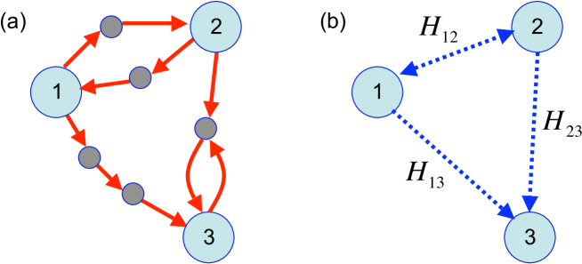
Figure 6: Schematic coarse-graining of a network of reactions. (a) This network has $M=10$ reactions (red arrows) and $N=8$ species, of which three are slow (large circles), and five are fast (small circles). (b) Dynamics of each fast node can be integrated out, leaving effective, coarse-grained, pairwise fluxes among the slow nodes. The fluxes along entire pathways connecting the slow pairs (blue arrows) are labeled by the corresponding effective Hamiltonians $H_{\mu\nu}$. Note that, for reversible pathways ($H_{12}$ in our example), the flux may be positive or negative (two-sided arrow), and it is strictly non-negative for the irreversible pathways (one-sided arrows).

At intermediate time scales, $\delta t$, many fast reactions connecting various slow variables can be considered statistically independent. Therefore, in the path integral, every separate chain of reactions that connects two slow variables simply adds a separate contribution to the effective Hamiltonian. Namely, let’s enumerate slow chemical species by $\mu,\nu,\dots$. Chains of fast reactions connecting them can be marked by pairs of indexes, e.g., $\mu\nu$ (cf. Fig.6). An entire such chain will contribute a single effective Hamiltonian term, $H_{\mu\nu}(\{N\},\{\chi\},\{\chi_{C}\})$, to the full CGF of the slow fluxes, where $\{N\}$, $\{\chi\}$, and $\{\chi_{C}\}$ are the set of the slow species and the conjugate, counting variables. If necessary, the geometric correction to the CGF, ${\mathcal{S}}_{\rm geom}^{\mu\nu}(\{N\},\{\chi\},\{\chi_{\rm C}\})$, can also be written out. Overall,

$${\mathcal{S}}(\{\chi_{\rm C}\},T)=\sum\limits_{\mu<\nu}{\mathcal{S}}_{\rm geom}^{\mu\nu}(\{N(t)\},\{\chi(t)\},\{\chi_{C}\},T)\\ +\int\limits_{0}^{T}dt\left[\sum\limits_{\mu}i\chi_{\mu}\dot{N}_{\mu}+\sum\limits_{\mu<\nu}H_{\mu\nu}(\{N(t)\},\{\chi(t)\},\{\chi_{\rm C}\})\right].$$ (21)

This expression provides for the following coarse-graining procedure. First, one finds a time scale $\delta t$, small enough for the slow species to be considered as almost static, and yet fast enough for the fast ones to equilibrate. If the fast species consist only of a few degrees of freedom, like in the case of a single enzyme, one can derive the CGF of the transformations mediated by these species either by using techniques presented in this article (cf. Methods: Coarse-graining the Michaelis Menten reaction), or discussed previously nazarov-03 ; gopich-06 ; sinitsyn-07epl . If instead the fast species are mesoscopic, one can use the stochastic path integral technique to derive the CGF by analogy with Step 2 of this article.

At the next step, these expressions for the CGFs of the fast species are incorporated into the stochastic path integral over the abundances of the slow variables. For this, one writes down the the full effective Hamiltonian, Eq. (21), assumes adiabatic evolution, and solves the ensuing saddle point equations. The extremum of the effective Hamiltonian determines the cumulant generating function. For hierarchies of time scales, this reduction procedure is repeated at every level of the hierarchy.

III Discussion

As biology continues to undergo the transformation from a qualitative, descriptive science to a quantitative one, it is expected that more and more rigorous analysis techniques developed in physics, chemistry, mathematics, and engineering will find suitable applications in the biological domain. This article represents one such example, where adiabatic approach, paired with the stochastic path integral formalism of mesoscopic statistical physics, allows one to coarse-grain stochastic biochemical kinetics systems.

For stiff systems with a pronounced separation of time scales, our technique eliminates relatively fast variables. It reduces stochastic networks to only the relatively slow species, coupled by complex interactions that accounts for the decimated nodes. The simplified system is smaller, non-stiff, and hence easier to analyze and simulate, resulting, in particular, in orders of magnitude improvement in the computational complexity of the simulations. Thus we believe that the approach has a potential to revolutionize the field of simulations in systems biology, at least for systems with the separation of time scales.

Fortunately, such separation occurs more prominently in Nature than one would intuitively suspect. Consider for example, the system given in Fig. 7, briefly mentioned in the Introduction. A molecule must be modified on $n$ sites in an arbitrary order to move from the inactive ($0,0,\ldots,0$) to the active ($1,1,\ldots,1$) state. The kinetic diagram for this system is an $n$-dimensional hypercube, and the number of states of the molecule with $m$ modified sites is ${n\choose m}$. Therefore, if the total number of molecules is $N$, then a typical $m$ times modified state will have $N_{m}=N/{n\choose m}$ molecules in it. This number may be quite small, ensuring the need for a full stochastic analysis. More importantly, it is quite different from either $N_{m-1}$ or $N_{m+1}$, e.g., $N_{m}/N_{m+1}=(m+1)/(n-m)$. As we discussed at length above, different occupancies result in the separation of time scales, and, on practice, the adiabatic approximation works quite well when this separation is a factor of only a few.

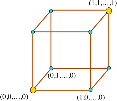
Figure 7: A molecule must be modified on $n$ sites (here $n=3$) in an arbitrary order to get activated. 0 and 1 indicate a non-modified/modified site, respectively. The number of states with $m\leq n$ modified sites is quite different for different $m$’s, which allows for a separation of time scales, as explained in the text.

In addition to the analysis and simulations, our adiabatic path integral-based coarse-graining scheme simplifies interpretation and understanding. For example, in certain cases, the Fano factor of the complex $S_{\rm B}\to P$ reaction, Eq. (15), approaches unity, suggesting a simplified, yet rigorous, interpretation with the entire reaction replaced by a simple Poisson step. Hence the list of relevant, important parameters may be smaller than suggested by the ab initio description of the system, aiding the understanding of the involved processes and decreasing the effective number of biochemical parameters that must be measured experimentally. Recent theoretical analysis suggests that this may be a universal property of biochemical networks sloppy ; ziv , with larger networks having proportionally fewer relevant parameters. Thus one may hope that the rigorous identification of the relevant degrees of freedom presented here will become even more powerful as larger, more realistic systems are considered.

We demonstrated the strength of our coarse-graining approach in analytical calculations of the Fano factor for the model system (relevant for single molecule experiments), and in numerical simulations, where the method substantially decreased the computational complexity. While impressive, this is still far from being able to coarse-grain large, cellular scale reaction networks. However, we believe that some important properties of our approach suggest that it may serve as an excellent starting point. Namely,

• We reduce a system of stochastic differential equations to a similar number of deterministic ones, which is a substantial simplification (see Methods).

• Our method can operate with arbitrarily long series of moments of the whole probability distribution of reaction events; i.e., it keeps track of mesoscopic fluctuations and even of rare events elgart-04 .

• The technique is very suitable for stiff systems, allowing to reduce the complexity by means of standard adiabatic approximations, well developed in classical and quantum physics.

• The stochastic path integral approach can deal with species that have copy numbers of order unity, which are ubiquitous in biological systems. This is not true for many other coarse-graining techniques.

• Finally, unlike many previous approaches, the stochastic path integral is rigorous, can be justified mathematically, and allows for controlled approximations.

In the forthcoming publications, we expect to show how these advantageous properties of the adiabatic path integral technique allow to coarse-grain many standard small and medium-sized biochemical networks.

IV Methods

IV.1 Moments generating functions for elementary chemical reactions

If during a time interval $\delta t$ the rate of an elementary chemical reaction is (almost) constant, then all reaction events are independent, and their number can be approximated as a Poisson variable. In its turn, the CGF of a Poisson variable is

$${\mathcal{S}}(\chi)=k(e^{i\chi}-1)\delta t,$$ (22)

where $k$ is the Poisson rate.

In our case, Fig. 2, two reactions satisfy these constraints for $\tau_{E}\ll\delta t\ll\tau_{M}$: substrate binding and unbinding to/from the membrane. Therefore, for these reactions we have:

$${\mathcal{S}}_{1}(\chi) = q_{0}S_{\rm B}(t)(e^{i\chi}-1)\delta t,$$ (23)

$${\mathcal{S}}_{2}(\chi) = qS_{\rm M}(t)(e^{i\chi}-1)\delta t.$$ (24)

IV.2 Coarse-graining the Michaelis-Menten reaction

Consider the $S_{\rm M}\to P$ reaction, described mathematically as in Eq. (1):

$$S_{\rm M}+E\xrightleftharpoons[k_{-1}]{k_{1}S_{\rm M}}C\xrightarrow{k_{2}}E+P.$$ (25)

The probabilities of transitions between bound ($P_{\rm b}$) and unbound ($P_{\rm u}$) states of the enzyme are given by a simple two state Markov process

$$\frac{d}{dt}\left[\begin{array}[]{l}P_{\rm u}\\ P_{\rm b}\end{array}\right]=-\left[\begin{array}[]{ll}\,\,\,\,k_{1}S_{\rm M}&-k_{-1}-k_{2}\\ -k_{1}S_{\rm M}&\,\,\,\,k_{-1}+k_{2}\end{array}\right]\left[\begin{array}[]{l}P_{\rm u}\\ P_{\rm b}\end{array}\right],$$ (26)

where $P_{\rm u}+P_{\rm b}=1$.

Lets introduce the MGF for the number of $S_{\rm M}\to P$ transitions,

$${\mathcal{Z}}_{3}(\chi,\delta t)=e^{{\mathcal{S}}_{3}(\chi)}=\sum_{n=0}^{\infty}P(\delta Q_{3}=n|\delta t)e^{in\chi},$$ (27)

Here $\delta Q_{\mu}$ stands for a charge transferred over time $\delta t$ in a reaction $\mu$, and $\mu=3$ is the MM reaction in toy model, Fig. 2. Using Eqs. (26, 27), one can show gopich-03 ; nazarov-03 ; gopich-06 ; sinitsyn-07prl , that ${\mathcal{Z}}_{3}(\chi,\delta t)$ satisfies a Schrödinger-like equation with a $\chi$-dependent Hamiltonian, leading to a formal solution

$${\mathcal{Z}}_{3}(\chi,\delta t)={\bf 1}^{+}\left(e^{-\hat{H}_{\rm MM}(\chi,t)\delta t}\right){\bf p}(t_{0}),$$ (28)

where ${\bf 1}^{+}=(1,1)$ is the unit vector, ${\bf p}(t_{0})$ is the probability vector of initial enzyme states, and

$$\hat{H}_{\rm MM}(\chi) =\left[\begin{array}[]{cc}k_{1}N_{s}&-k_{-1}-k_{2}e^{i\chi}\\ -k_{1}N_{s}&k_{-1}+k_{2}\end{array}\right].$$ (31)

The Hamiltonian, analogous to Eq. (31), can be derived for a very wide class of kinetic schemes nazarov-03 ; gopich-06 ; sukhorukov-07 ; sinitsyn-07prb , allowing for a relatively straightforward extension of our methods.

The solution, Eq. (28), can be simplified considerably if the reaction is considered in a quasi-steady state approximation, that is $P_{u}$ is equilibrated at a current value of the other parameters. This means that the time on which the reaction is being studied, $\delta t\sim\tau_{\rm M}$, is much larger than a characteristic time of a single enzyme turnover, $\tau_{\rm E}$, so we can consider $\delta t\to\infty$ in Eq. (28). Then only the eigenvalue $\lambda_{0}(\chi)$ of the Hamiltonian $\hat{H}_{\rm MM}(\chi)$ with the smallest real part is relevant, and

$${\mathcal{Z}}_{3}(\chi,\delta t)=e^{-\lambda_{0}(\chi)\delta t}.$$ (32)

It is possible to incorporate a slow time dependence of the parameters into this answer. By analogy with the quantum mechanical Berry phase sinitsyn-07epl ; sinitsyn-07prl ; sinitsyn-07prb , the lowest order non-adiabatic correction can be expressed as a geometric phase

$${\mathcal{Z}}_{3}(\chi)=e^{{\mathcal{S}}_{3}(\chi)}=e^{\int_{{\bf c}}{\bf A\cdot dk}-\int dt\lambda_{0}(\chi,t)},$$ (33)

where ${\bf A}=\langle u_{0}(\chi)|\partial_{{\bf k}}u_{0}(\chi)\rangle$, ${\bf k}$ is the vector in the parameter space, which draws a contour ${\bf c}$ during the parameter evolution, and $\langle u_{0}(\chi)|$ and $|u_{0}(\chi)\rangle$ are the left and the right eigenvectors of $\hat{H}_{\rm MM}(\chi,t)$ corresponding to the instantaneous eigenvalue $\lambda_{0}(\chi,t)$. The first term in Eq. (33) is the geometric phase, which is responsible for various ratchet-like fluxes sinitsyn-07epl ; ohkubo-07aa ; astumian-07pnas .

After elimination of the fast degrees of freedom, the geometric phase gives rise to magnetic field-like corrections to the evolution of the slow variables. However, since these corrections depend on time derivatives of the slow variables, they usually are small and can be disregarded, unless they break some important symmetry, such as the detailed balance sinitsyn-07prl ; astumian-07pnas , or the leading non-geometric term is zero. In our model, the geometric effects are negligible when compared to the dominant contribution when $\tau_{\rm E}/\tau_{\rm M}\sim 1/S_{\rm M}$, and we deemphasize them in most derivations. However, we keep the geometric terms in several formal expressions for completeness, and the reader should be able to track its effects if desired.

Reading the value of $\lambda_{0}(\chi)$ from Ref. sinitsyn-07epl, , we conclude that the number of particles converted from $S_{\rm M}$ to $P$ over time $\delta t$, $\tau_{\rm E}\ll\delta t\lesssim\tau_{\rm M}$ in the adiabatic (MM) limit is described by the following CGF:

$${\mathcal{S}}_{3}(\chi,\delta t)={\mathcal{S}}_{\rm geom}(\chi,S_{\rm M},\dot{S}_{\rm M})+\\ \frac{\delta t}{2}\left[-(k_{-1}+k_{2}+S_{\rm M}k_{1})+\sqrt{(k_{-1}+k_{2}+S_{\rm M}k_{1})^{2}+4S_{\rm M}k_{1}k_{2}(e^{i\chi}-1)}\right].$$ (34)

IV.3 Simulations with near-Gaussian distributions

A probability distribution $P(\delta Q)$ with known cumulants $c_{1}$, $c_{2}$,…, can be written as a limited Gram-Charlier expansion edgeworth

$$P(\delta Q)\approx\Psi(\delta Q,c_{1},c_{2})\left[1+\frac{c_{3}(y^{3}-y)}{6c_{2}^{3/2}}+\frac{c_{4}(y^{4}-6y^{2}+3)}{24c_{2}^{2}}+\frac{c_{3}^{2}(y^{6}-15y^{4}+45y^{2}-15)}{72c_{2}^{3}}+\cdots\right],$$ (35)

where $y=(\delta Q-c_{1})/\sqrt{c_{2}}$ and $\Psi(\delta Q,c_{1},c_{2})$ is the Gaussian density with the mean $c_{1}$ and the variance $c_{2}$. The leading term in the series is a standard Gaussian approximation, and the subsequent terms correctly account for skewness, kurtosis, etc. Note that if all cumulants scale similarly, as is true for our near-Gaussian case, then the terms in the series become progressively smaller, ensuring good approximations in practice.

While the Gram-Charlier expansion provides a reasonable approximation to $P$, generation of random samples from such a non-Gaussian distribution is still a difficult task. However, if, instead of the random numbers per se, the goal is to calculate the expectation of some function $f(\delta Q)$ over the distribution $P$, $\langle f(\delta Q)\rangle_{P}$, then the importance sampling technique imp-sampl can be used. Specifically, we generate a Gaussian random number $\delta Q$ according to $\Psi(\delta Q,c_{1},c_{2})$ and define its importance factor according to its relative probability in the reference normal distribution and the desired Gram-Charlier approximation

$$\eta=\frac{P(\delta Q)}{\Psi(\delta Q,c_{1},c_{2})}.$$ (36)

After generating $N$ such random numbers $\delta Q_{\nu}$, $\nu=1,\dots,N$, we obtain the needed expectation values as

$$\langle f\rangle_{P}=\frac{\sum_{\nu=1}^{N}\eta_{\nu}f(\delta Q_{\nu})}{\sum_{\nu=1}^{N}\eta_{\nu}}.$$ (37)

If a current random number draw represents just one reaction in a larger reaction network, then the overall importance factor of a Monte Carlo realization is a product of the factors for each of the random numbers drawn within it.

Note that the method reduces the complexity of simulations to that of a simple Gaussian, Langevin process with a small burden of (a) evaluating an algebraic expression for the Gram-Charlier expansion, and (b) keeping track of the importance factor for each of the Monte Carlo runs. Yet, at least in principle, this small computational investment allows to account for an arbitrary number of cumulants of the involved variables. To illustrate this, in Fig. 8, we compare the Gram-Charlier-based, importance-sampling corrected simulations of the MM reaction flux to the exact results in Results: Step 1. Introducing just the third and the fourth cumulant makes the simulations almost indistinguishable from the exact results.

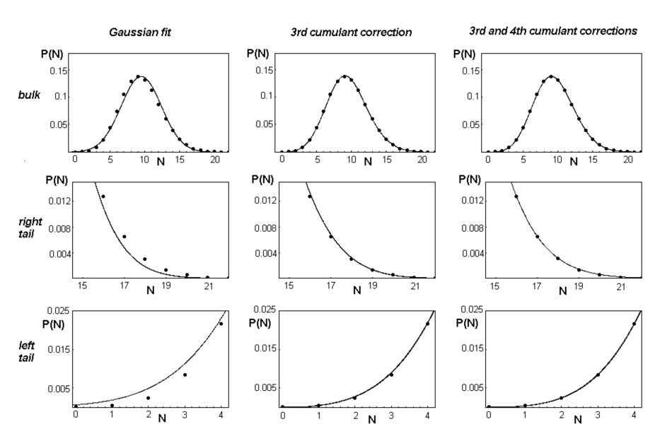
Figure 8: Comparison of an exact discrete distribution of product molecules generated by MM-enzyme (discrete points), with the fit by continuous approximation by leading terms of Gram-Charlier series. Left column compares the exact result to the Gaussian approximation with the same first two cumulants. Central column shows improvement of the fit due to inclusion of the third cumulant correction. Including the fourth cumulant (right column) makes the approximation and the exact result virtually indistinguishable. For these plots, we used $S_{\rm M}=140={\rm const}$, $k_{1}=0.02$, $k_{-1}=2.$, $k_{2}=1.$, $q=0.01$, and time step size $\delta t=35$ (see Introduction: The model and Results for explanation of the parameters).

We end this section with a note of caution: the Gram-Charlier series produces approximations that are not necessarily positive and hence are not, strictly speaking, probability distributions. However, the leading Gaussian term decreases so fast that this may not matter in practice. Indeed, in our analysis, we simply rejected any random number that had a negative importance correction, and the agreement with the analytical results was still superb.

However, this simplistic solution becomes inadequate for lengthy simulations, where the probability that one of random numbers in a long chain of events falls into a badly approximated region of the distribution approaches one. Then the importance factor of the entire chain of events becomes incorrect, spoiling the convergence. In these situations, other approaches for generating random numbers should be used. A prominent candidate is the well-known acceptance-rejection method rejection . Since the true distributions we are interested in are near-Gaussian, a Gaussian with a slightly larger variance will be an envelope function for the Gram-Charlier approximation to the true distribution. Then the average random number acceptance probability will be similar to the ratio of the true and the envelope standard deviations, and it can be made arbitrary high. Then the rejection approach will require just a bit more than one normal and one uniform random number to generate a single sample from the underlying Gram-Charlier expansion. The orders-of-magnitude gain due to the transition to the coarse-grained description should fully compensate for this loss. Note that, in this case, the negativity of the series is not a problem since it will lead to an incorrect rejection of a single, highly improbable sample, rather than an entire sampling trajectory.

IV.4 Coarse-graining all membrane reactions

To complete the coarse-graining step that connects Figs. 3(b) and 3(c), we look for the MGF of the total number of products $Q_{\rm P}$ produced over time $T\sim\tau_{B}$:

$${\mathcal{Z}}(\chi_{C})=e^{{\mathcal{S}}(\chi_{C})}=\sum_{Q_{P}=0}^{\infty}P(Q_{\rm P}|T)e^{iQ_{\rm P}\chi_{C}}.$$ (38)

For this, we discretize the time into intervals $t_{k}$ of durations $\delta t$, and we introduce random variables $\delta Q_{\mu}(t_{k})$ ($\mu=1,2,3$), which represent the number of each of the three different reactions in Fig. 3(b) (membrane binding, unbinding, and MM conversion) during each time interval. The probability distributions of $\delta Q_{\mu}(t_{k})$ are given by inverse Fourier transforms of the corresponding MGFs:

$$P(\delta Q_{\mu}(t_{k}))=\frac{1}{2\pi}\int d\chi_{\mu}(t_{k})e^{-i\chi_{\mu}(t_{k})\delta Q_{\mu}(t_{k})+H_{\mu}(\chi_{\mu}(t_{k}),S_{\rm B}(t_{k}))\delta t},$$ (39)

where the CGF is

$${\mathcal{S}}_{\mu}(\chi,S_{\rm B})=H_{\mu}(\chi,S_{\rm B})\delta t.$$ (40)

Following pilgram-03 ; pilgram-04 ; sukhorukov-04 ; sinitsyn-07prl , the MGF of the total number of product molecules created during time interval $(0,T)$ is given by the path integral over all possible trajectories of $\delta Q_{\mu}(t_{k})$ and $S_{\rm M}(t_{k})$:

$$e^{{\mathcal{S}}(\chi_{\rm C},T)}=\langle e^{i\chi_{\rm C}Q_{\rm P}}\rangle=\int DS_{\rm M}(t_{k})\prod_{k}\prod_{\mu}\int D\delta Q_{\mu}(t_{k})\ P[\delta Q_{\mu}(t_{k})]e^{i\chi_{C}\sum_{t_{k}}\delta Q_{3}(t_{k})}\\ \times\delta(S_{\rm M}(t_{k+1})-S_{\rm M}(t_{k})-\delta Q_{1}(t_{k})+\delta Q_{2}(t_{k})+\delta Q_{3}(t_{k})).$$ (41)

Here we used the fact that $Q_{\rm P}=\sum\limits_{k}\delta Q_{3}(t_{k})$.

The $\delta$-function in the path integral expresses the conservation law for the slowly changing number of substrate molecules $S_{\rm M}$. We rewrite it as an inverse Fourier transform,

$$\delta(S_{\rm M}(t_{k+1})-S_{\rm M}(t_{k})-\delta Q_{1}(t_{k})+\delta Q_{2}(t_{k})+\delta Q_{3}(t_{k}))=\\ \frac{1}{2\pi}\int_{-\pi}^{+\pi}d\chi_{\rm M}(t_{k})\exp{\{i\chi_{\rm M}(t_{k})\left[S_{\rm M}(t_{k+1})-S_{\rm M}(t_{k})-\delta Q_{1}(t_{k})+\delta Q_{2}(t_{k})+\delta Q_{3}(t_{k})\right]\}},$$ (42)

and we substitute the expression together with Eq. (39) into Eq. (41). Then the integration over $\delta Q_{\mu}(t)$ produces new $\delta$-functions over $\chi_{\mu}$, which, in turn, are removed by integration over $\chi_{\mu}(t_{k})$. This leads to an expression for the MGF:

$$e^{{\mathcal{S}}(\chi_{\rm C},T)}=\int DS_{\rm M}\int D\chi_{\rm M}\exp{\int_{0}^{T}dt[i\chi_{\rm M}\dot{S}_{\rm M}+H(S_{\rm M},\chi_{\rm M},\chi_{\rm C})]},$$ (43)

where

$$H(S_{\rm M},\chi_{\rm M},\chi_{\rm C})= H_{1}(-\chi_{\rm M},S_{\rm M},t)+H_{2}(\chi_{\rm M},S_{\rm M},t)+H_{3}(\chi_{\rm M}+\chi_{\rm C},S_{\rm M},t)$$ (44)

$$= q_{0}S_{\rm B}(e^{-i\chi_{\rm M}}-1)+S_{\rm M}q(e^{i\chi_{\rm M}}-1)+$$

$$\frac{1}{2}\left[-(k_{-1}+k_{2}+S_{\rm M}k_{1})+\sqrt{(k_{-1}+k_{2}+S_{\rm M}k_{1})^{2}+4S_{\rm M}k_{1}k_{2}(e^{i\chi_{\rm M}+\chi_{\rm C}}-1)}\right]$$ (45)

Notice that, unlike in the original work on the stochastic path integral pilgram-03 , which assumed all component reactions to be Poisson, here $H_{3}$ is the CGF of the entire complex MM reaction. This we read as the coefficient in front of $\delta t$ in Eq. (34), and it is clearly non-Poisson. This ability to include subsystems with small number of degrees of freedom, such as a single Michaelis-Menten enzyme or a stochastic gene expression, into coarse-graining mechanism based on the the stochastic path integral techniques opens doors to application of the method to a wide variety of coarse-graining problems.

Since $S_{\rm M}\gg 1$, this path integral is dominated by the classical solution of the equations motion (i. e., the saddle point), which, near the steady state, are

$$\dot{S}_{\rm M}=0, \dot{\chi}_{\rm M}=0,$$ (46)

$$\frac{\partial H}{\partial\chi_{\rm M}}=0, \frac{\partial H}{\partial S_{\rm M}}=0.$$ (47)

Let $\chi_{\rm cl}(\chi_{\rm C})$ and $S_{{\rm M},{\rm cl}}(\chi_{\rm C})$ solve Eq (47). Then the cumulants generating function in the quasi-steady state approximation is

$${\mathcal{S}}(\chi_{\rm C},T)=T\,H(S_{\rm M,cl}(\chi_{\rm C}),\chi_{\rm cl}(\chi_{\rm C}),\chi_{\rm C})$$ (48)

This formally completes the last step of the coarse-graining by deriving the cumulant generating function for the number of complex $S_{\rm B}\to P$ transformation over long times.

IV.5 Simulations details

All computer simulations were performed using Fortran 90 code, on a single processor AMD Barton 2500 (1.83 GHz), and operating system Windows 2000.

- (1) D.S. English, A. Furube, and P.F. Barbara, Single-molecule spectroscopy in oxygen-depleted polymer films, Chem. Phys. Lett 324, 15 (2000).
- (2) M. Orrit, Photon Statistics in Single Molecule Experiments, Single Mol. 3, 255 (2002).
- (3) I.V. Gopich and A. Szabo, Statistics of transition in single molecule kinetics, J. Chem. Phys. 118, 454 (2003).
- (4) B.P. English, et al., Ever-fluctuating single enzyme molecules: Michaelis-Menten equation revisited. Nat. Chem. Biol. 2, 87 (2006).
- (5) X. Xue, F. Liu, and Z. Ou-Yang, Single molecule Michaelis-Menten equation beyond quasistatic disorder Phys. Rev. E 74, 030902(R) (2006).
- (6) S. Chaudhury and B.J. Cherayil, Dynamic disorder in single-molecule Michaelis-Menten kinetics: The reaction-diffusion formalism in the Wilemski-Fixman approximation. J. Chem. Phys. 127, 105103 (2007).
- (7) I.G. Darvey, B.W. Ninham and P.J. Staff, Stochastic Models for Second-Order Chemical Reaction Kinetics. The Equilibrium State. J. Chem. Phys. 45, 2145 (1966).
- (8) J.E.M. Hornos, et al., Self-regulating gene: An exact solution, Phys. Rev. E 72, 051907 (2005).
- (9) S. Iyer-Biswas, F. Hayot, and C. Jayaprakash, Transcriptional pulsing and consequent stochasticity in gene expression. Preprint, http://arXiv.org/abs/0711.1141 (2007).
- (10) M. Sasai and P.G. Wolynes, Stochastic gene expression as a many-body problem. Proc. Natl. Acad. Sci. (USA) 100, 2374 (2003).
- (11) Y. Lan, P.G. Wolynes, and G.A. Papoian, J. Chem. Phys. 125, 124106 (2006).
- (12) W.S. Hlavacek et al., Rules for Modeling Signal-Transduction Systems. Sci. STKE, 344 (2006).
- (13) O.G. Berg, A model for the statistical fluctuations of protein numbers in a microbial population. J. Theor. Biol., 71, 587 (1978).
- (14) H. McAdams and A. Arkin, Stochastic mechanisms in geneexpression Proc. Natl. Acad. Sci. (USA) 94, 814 (1997).
- (15) J. Paulsson and M. Ehrenberg, Random Signal Fluctuations Can Reduce Random Fluctuations in Regulated Components of Chemical Regulatory Networks. Phys. Rev. Lett. 84, 5447 (2000).
- (16) P. Cluzel, M. Surette and S. Leibler, An ultrasensitive bacterial motor revealed by monitoring signaling proteins in single cells. Science 287, 1652 (2000).
- (17) M. Elowitz, A. Levine, E. Siggia and P. Swain, Stochastic Gene Expression in a Single Cell. Science, 297, 1183 (2002).
- (18) J.M. Raser, E.K. O’Shea, Noise in gene expression: Origins, consequences, and control. Science 304, 1811 (2004).
- (19) W. Bialek and S. Setayeshgar, Physical limits to biochemical signaling. Proc. Natl. Acad. Sci. (USA) 102, 10040 (2005).
- (20) L.P. Kadanoff and A. Houghton, Numerical evaluations of the critical properties of the two-dimensional Ising model. Phys. Rev. B 11, 377 (1975).
- (21) Shang-Keng Ma, M. K. Fung, Statistical Mechanics (World Scientific, 1984).
- (22) L. Michaelis and M.L. Menten, Die Kinetik der Invertinwerkung. Biochemische Zeitschrift. Biochem. Z. 49, 333 (1913).
- (23) M. Samoilov, A.P. Arkin and J. Ross, Signal Processing by Simple Chemical Systems. J. Phys. Chem. A 106, 10205 (2002).
- (24) C.V. Rao and A.P. Arkin, Stochastic chemical kinetics and the quasi-steady-state assumption: application to the Gillespie algorithm. J. Chem. Phys. 118, 4999 (2003).
- (25) M. Samoilov, S. Plyasunov, and A.P. Arkin, Stochastic amplification and signaling in enzymatic futile cycles through noise-induced bistability with oscillations. Proc. Natl. Acad. Sci. (USA) 102, 2310 (2005).
- (26) I.V. Gopich and A. Szabo, Theory of the statistics of kinetic transitions with application to single-molecule enzyme catalysis. J. Chem. Phys. 124, 154712 (2006).
- (27) N.A. Sinitsyn and I. Nemenman, Berry phase and pump effect in stochastic chemical kinetics. EPL 77, 58001 (2007).
- (28) S. Pilgram et al., Stochastic Path Integral Formulation of Full Counting Statistics. Phys. Rev. Lett. 90, 206801 (2003).
- (29) A.N. Jordan, E.V. Sukhorukov and S. Pilgram, Fluctuation statistics in networks: A stochastic path integral approach. J. Math. Phys. 45, 4386 (2004).
- (30) V. Elgart and A. Kamenev, Rare event statistics in reaction-diffusion systems . Phys. Rev. E 70, 041106 (2004).
- (31) N.A. Sinitsyn and I. Nemenman, Universal Geometric Theory of Mesoscopic Stochastic Pumps and Reversible Ratchets. Phys. Rev. Lett. 99, 220408 (2007).
- (32) Jean Zinn-Justin,Quantum Field Theory and Critical Phenomena (Oxford University Press, USA, 2002).
- (33) Y. Cao, D.T. Gillespie, and L.R. Petzold, Accelerated stochastic simulation of the stiff enzyme-substrate reaction. J. Chem. Phys. 123, 054104 (2005).
- (34) Y. Cao, D.T. Gillespie, and L.R. Petzold, Efficient step size selection for the tau-leaping simulation method. J. Chem. Phys. 124, 4 (2006).
- (35) P. Detwiler, S. Ramanathan, A. Sengupta and B. Shraiman. Engineering aspects of enzymatic signal transduction: Photoreceptors in the retina. Biophys. J. 79 2801 (2000).
- (36) C. Wu, H.J. Cha, J.J. Valdes, W.E. Bentley, GFP-visualized Immobilized Enzymes: Degradation of Paraoxon via Organophosphorous Hydrolase in a Packed Column. Biotechn. Bioeng. 77, 212 (2001).
- (37) D.T. Gillespie, Exact Stochastic Simulation of Coupled Chemical Reactions. J. Phys. Chem. 81, 2340 (1977).
- (38) N. Le Novre and T.S. Shimizu, STOCHSIM: modelling of stochastic biomolecular processes. Bioinformatics 17, 575 (2001).
- (39) Melvin Lax, Wei Cai, and Min Xu,”Random Processes in Physics and Finance” (Oxford University Press, USA 2006).
- (40) S. Blinnikov and R. Moessner, Expansions for nearly Gaussian distributions. Astron. Astrophys. Suppl. Ser. 130, 193 (1998).
- (41) R. Srinivasan, Importance sampling - Applications in communications and detection (Springer-Verlag: Berlin, 2002).
- (42) D. Stekel and D. Jenkins, Strong negative self regulation of Prokaryotic transcription factors increases the intrinsic noise of protein expression, BMC Syst. Biol. 2, 1 (2008).
- (43) D.A. Bagrets and Y.V. Nazarov, Full counting statistics of charge transfer in Coulomb blockade systems. Phys. Rev. B 67, 085316 (2003).
- (44) R. Gutenkunst, J. Waterfall, F. Casey, K Brown, C. Myers, J. Sethna, Universally Sloppy Parameter Sensitivities in Systems Biology. PLoS Comput. Biol. 3, e189 (2007).
- (45) E. Ziv, I. Nemenman, and C. Wiggins, Optimal information processing in small stochastic biochemical networks. PLoS ONE 2, e1077 (2007).
- (46) E.V. Sukhorukov, A.N. Jordan, Stochastic Dynamics of a Josephson Junction Threshold Detector. Phys. Rev. Lett. 98, 136803 (2007).
- (47) N.A. Sinitsyn, Reversible stochastic pump currents in interacting nanoscale conductors. Phys. Rev. B 76, 153314 (2007).
- (48) J. Ohkubo, The stochastic pump current and the non-adiabatic geometrical phase. J. Stat. Mech. P02011 (2008).
- (49) R.D. Astumian, Adiabatic operation of a molecular machine. Proc. Natl. Acad. Sci. (USA) 104, 19715 (2007).
- (50) A.N. Jordan and E.V. Sukhorukov, Transport Statistics of Bistable Systems. Phys. Rev. Lett. 93, 260604 (2004).
- (51) J. von Neumann, Various techniques used in connection with random digits. Monte Carlo methods. Nat. Bureau Standards 12, 36 (1951).