Evolutionary Model of Species Body Mass Diversification

Abstract

We present a quantitative model for the biological evolution of species body masses within large groups of related species, e.g., terrestrial mammals, in which body mass $M$ evolves according to branching (speciation), multiplicative diffusion, and an extinction probability that increases logarithmically with mass. We describe this evolution in terms of a convection-diffusion-reaction equation for $\ln M$. The steady-state behavior is in good agreement with empirical data on recent terrestrial mammals, and the time-dependent behavior also agrees with data on extinct mammal species between $95$ – $50$ Myr ago.

Animals—both extant and extinct—exhibit an enormously wide range of body sizes. Among extant terrestrial mammals, the largest is the African savannah elephant (Loxodonta africana africana) with a mass of $10^{7}\,\mathrm{g}$, while the smallest is Remy’s pygmy shrew (Suncus remyi) at a diminutive $1.8\,\mathrm{g}$. Yet the most probable mass is $40\,\mathrm{g}$, roughly the size of the common Pacific rat (Rattus exulans), is only a little larger than the smallest mass. More generally, empirical surveys suggest that such a broad but asymmetric distribution in the number of species with adult body mass $M$ typifies many animal classes Stanley (1973); Kozłowski and Gawelczyk (2002); Allen et al. (2006); Carrano (2006); Meiri (2008), including mammals, birds, fish, insects, lizards and possibly dinosaurs.

What mechanisms cause species mass distributions to assume such a shape? A satisfactory answer would have wide implications for the evolution and distribution of the many other species characteristics that correlate with body mass, including life span, metabolic rate, and extinction risk Calder III (1984); Cardillo et al. (2005). Previous explanations for the species mass distribution focused on detailed ecological, environmental and species-interaction assumptions Allen et al. (2006). However, empirical data present confusing and often inconsistent support for these theories, and none explicitly address how species body mass distributions diversify in time.

In this Letter, we construct a physics-based convection-diffusion-reaction model to account for the evolution of the species mass distribution. The steady-state behavior of this model was recently solved to explain the species mass distribution for recent terrestrial mammals and birds Clauset and Erwin (2008); Clauset et al. (2008), where recent is conventionally defined as within the past 50,000 years Smith et al. (2003). Here we substantially extend this approach to give predictions on mammalian body mass evolution that are in good agreement with fossil data. This model can further be used to estimate the historical rates of body mass diversification from fossil data, which are otherwise estimated using ad hoc techniques. To illustrate this application, we estimate body mass diversification rates from our fossil data, which are in good agreement with estimates of genetic diversification from molecular clock methods Springer et al. (2003). Although our focus is on terrestrial mammal evolution, this model can, in principle, be applied to any group of related species.

Let $c(x,t)$ denote the number (density) of species having logarithmic mass $x=\ln M$ at a time $t$; we use $x$ as the basic variable in keeping with widespread usage in the field Clauset and Erwin (2008). Our model incorporates three fundamental and empirically-supported features of biological evolution.

1. Branching multiplicative diffusion Stanley (1973); Clauset and Erwin (2008): each species of mass $M$ produces descendant species (cladogenesis) with masses $\lambda M$, where $\lambda$ is a random variable, and the sign of the average $\langle\ln\lambda\rangle$ denotes bias toward larger or smaller descendants. Empirical evidence Clauset and Erwin (2008) suggests that $\langle\ln\lambda\rangle>0$ (known as Cope’s rule Stanley (1973)) for terrestrial mammals.

2. Species become extinct independently, and with a probability that increases weakly with mass Liow et al. (2008).

3. No species can be smaller than a mass $M_{\min}$, due, for example, to metabolic constraints West et al. (2002).

The production of descendant species corresponds to growth in the number of species at a rate $k$ that is proportional to the density $c$ itself. Similarly, the probability $p(x)$ that a species of logarithmic mass $x$ becomes extinct may also be represented by a loss term that is proportional to $c$, but with a weak mass dependence Clauset and Erwin (2008). We make the simple choice of linear dependence $p(x)=A+Bx$ (but see below). With these ingredients, $c(x,t)$ obeys the convection-diffusion-reaction equation in the continuum limit

$$\frac{\partial c}{\partial t}+v\frac{\partial c}{\partial x}=D\frac{\partial^{2}c}{\partial x^{2}}+(k-A-Bx)c\enspace,$$ (1)

with bias velocity $v=\langle\ln\lambda\rangle$ and diffusion coefficient $D=\langle(\ln\lambda)^{2}\rangle$, and where $k-A$ sets the absolute scale of species body mass frequencies.

To solve Eq. (1), we substitute the eigenfunction expansion $c(x,t)=\sum_{n}A_{n}\mathcal{C}_{n}(x)\,\mathrm{e}^{-\gamma_{n}t}$, which yields

$$-\frac{\gamma_{n}}{D}\mathcal{C}_{n}+\mu\mathcal{C}_{n}^{\prime}=\mathcal{C}_{n}^{\prime\prime}+(\alpha-\beta x)\mathcal{C}_{n}\enspace,$$ (2)

where the prime denotes differentiation with respect to $x$, $\mu=v/D$, $\alpha=(k-A)/D$, and $\beta=B/D$. We eliminate the first derivative term by introducing $\psi_{n}=\mathrm{e}^{-\mu x/2}\,\mathcal{C}_{n}$ and then we use the scaled variable $z=\beta^{1/3}x-\beta^{-2/3}\left(\alpha-\frac{\mu^{2}}{4}+\frac{\gamma_{n}}{D}\right)$ to transform Eq. (2) into Airy’s differential equation, $\psi^{\prime\prime}-z\psi=0$ Abramowitz and Stegun (1972), for each eigenfunction $\psi_{n}$. The general solution is $\psi(z)=a_{1}\,{\rm Ai}(z)+a_{2}\,{\rm Bi}(z)$, where Ai$(z)$ and Bi$(z)$ are the Airy functions; here the prime now denotes differentiation with respect to $z$. Since there can be no species with infinite mass and Bi$(z)$ diverges as $z\to\infty$, we set $a_{2}=0$, while $a_{1}$ is determined by the initial condition. (We could also incorporate a fixed maximum species body mass $M_{\max}$, but the analysis is more complicated without revealing additional insights.)

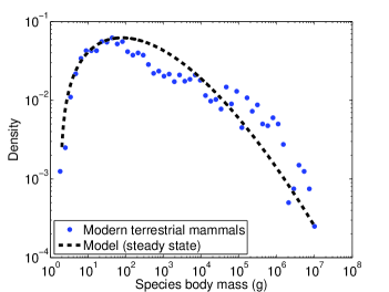
Figure 1: (color online) Steady-state solution of the model for the species body mass distribution and suitably binned empirical data for 4002 recent terrestrial mammals (shown as a normalized histogram with 50 logarithmically-spaced bins).

Since the species density vanishes at the minimum mass $M_{\min}$, the argument of $\psi_{n}$ must equal

$$z_{n}\!=\!\beta^{1/3}x_{\min}\!-\!\beta^{-2/3}\left(\!\alpha\!-\!\frac{\mu^{2}}{4}\!+\!\frac{\gamma_{n}}{D}\!\right)=z_{0}\!-\!\frac{\gamma_{n}}{D\beta^{2/3}}\enspace.$$ (3)

The functions $\psi_{n}={\rm Ai}(z_{n})$ form the complete set of states for the eigenfunction expansion Courant and Hilbert (1989). The first few zeros $z_{n}$ are at (roughly) $-2.3381$, $-4.0879$, $-5.5205$ and $-6.7867$ for $n=0,1,2,3$ Abramowitz and Stegun (1972). (For computing the distribution, we tabulated the first million zeros numerically using standard mathematical software.) The corresponding decay rates $\gamma_{n}$ are then given by $\gamma_{n}=D\,\beta^{2/3}(z_{0}-z_{n})$, with $\gamma_{0}=0$ to give the steady state solution Clauset et al. (2008). These rates form an increasing sequence so that the higher terms in the eigenfunction expansion decay more quickly in time. Finally, solving Eq. (3) for $\alpha$ and plugging the result into the definition of $z$, we can eliminate the scale parameter $\alpha$ and write $z=z_{n}+\beta^{1/3}(x-x_{\min})$. Thus each eigenfunction has the form

$$\mathcal{C}_{n}(x)\propto\mathrm{e}^{\mu x/2}\,{\rm Ai}\left[z_{n}+\beta^{1/3}(x-x_{\min})\right],$$ (4)

in which ${\rm Ai}(z)\sim\mathrm{e}^{-2z^{3/2}/3}$ for large $z$. The competition between this decay and the prefactor $\mathrm{e}^{\mu x/2}$ in $\mathcal{C}_{n}(x)$ contributes to the broadness of the species mass distribution and the location of the most probable mass (Fig. 1). Parenthetically, the asymptotic decay of the eigenfunctions depends only weakly on the form of the extinction probability $p(x)$. For instance, if we choose $p(x)=A+Bx^{\delta}$, then as $z\to\infty$, the eigenfunctions decay as $\mathrm{e}^{-z^{1+\delta/2}}$.

Figure 2: (color online) Data on species body mass for 569 North American terrestrial mammals Alroy (2008) from 95 – 50 Myr ago. Each horizontal segment represents a species, and endpoints denote its first and last appearance in the fossil record. The superimposed curve shows the average of $\ln M$ for these species (smoothed with an exponential kernel).

Suppose that a given group of animals began its evolutionary history with a single species of mass $M_{0}$ (initial condition $c(x,t=0)=\delta(x-x_{0})$, with $x_{0}=\ln M_{0}$), after which speciation occurs according to the dynamics of Eq. (1). We use the fact that the Airy differential equation is a Sturm-Liouville problem Courant and Hilbert (1989) so that the $\{\mathcal{C}_{n}\}$ form a complete and orthonormal set. Following the standard prescription to determine the coefficients of the eigenfunction expansion, the full time-dependent solution is

$$c(x,t)=\sum_{n}\mathcal{C}_{n}(x_{0})\mathcal{C}_{n}(x)\,\mathrm{e}^{-\gamma_{n}t}\enspace,$$ (5)

where each $\mathcal{C}_{n}(x)$ is given by Eq. (4). In the long-time limit, all the decaying eigenmodes with $n>0$ become negligible and the species mass distribution reduces to $c(x,t\to\infty)\propto\mathcal{C}_{0}(x)$.

We test our predictions for the species body mass distribution by comparing with available empirical data. In the steady state, our model is characterized by three parameters: $M_{\min}$, the mass of the smallest animal, $\mu$, which controls the tendency of descendant species to be larger or smaller than their ancestors, and $\beta$, which controls the dependence of the extinction rate on mass. The former two can be estimated directly from fossil data, while the latter is typically estimated by matching the steady-state solution to the recent data. For terrestrial mammals, we previously found $\mu\approx 0.2$, $\beta\approx 0.08$, while $M_{\min}\approx 2\,\mathrm{g}$ Clauset et al. (2008). Using these parameter values in the long-time limit, we obtain a good agreement between the predictions of the model and the species mass distribution of recent terrestrial mammals Smith et al. (2003) (Fig. 1).

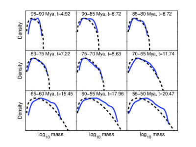
Figure 3: (color online) A comparison of our model predictions (dashed) from Eq. (5) and the mass distributions of extinct North American mammal species (solid) in nine consecutive time ranges. (To get reasonable results with sparse empirical data, we smooth the distributions with a Gaussian kernel.)

Our model also makes predictions about the way the body mass distribution changes over time, which can be tested with fossil data. Drawing on data from the best available source on the evolution of mammalian body masses Alroy (2008), we plot in Fig. 2 the durations and body masses of 569 extinct mammal species from 95 – 50 Myr ago. This period includes the Cretaceous-Paleogene (KP) boundary of 65.5 Myr ago that marks a mass extinction event during which more than 50% of then extant species became extinct, including non-avian dinosaurs—the dominant fauna for the preceding 160 Myr—and is the subject of many studies regarding the diversification of mammals. (The Cretaceous period is conventionally abbreviated “K,” after the German translation Kreide.)

Using the same model parameters as above, and setting $M_{0}=2\,\mathrm{g}$, the estimated size of the first mammal Luo et al. (2001), Fig. 3 shows good agreement between model predictions from Eq. (5) and empirical data from Fig. 2. To simplify the comparison, we divided the period from 95 – 50 Myr ago into nine bins of equal durations, and tabulated the distribution of species extant during each of these bins. In each of the nine panels of Fig. 3, we give both the historical time period and the corresponding model time that yields a good qualitative match to the data. (The fitting can be made more objective using standard techniques, but the results are largely the same.)

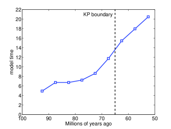
Figure 4: Estimated relation between model time to historical time, indicating that the broadening of the mammalian species mass distribution began approximately 10 Myr before the KP boundary when non-avian dinosaurs became extinct.

The relation between historical time and model time is itself interesting (Fig. 4). During the first 20 Myr (95 – 75 Myr ago), the species mass distribution is almost stationary, with model time advancing by only $\Delta t=2.30$; curiously, between 90 – 80 Myr ago, model time does not advance at all. This period of near stasis may indicate a lull in the evolutionary dynamics, perhaps due to implicit competition from larger species, e.g., dinosaurs. Over the next 20 Myr (75 – 55 Myr ago), however, the distribution broadens considerably (model time advancing by $\Delta t=10.74$), and comes to closely resemble the recent distribution (Fig. 1). This correspondence suggests that the diversification of mammalian body masses into their recent state began at least 75 Myr ago, roughly 10 Myr before the KP boundary and the extinction of the non-avian dinosaurs. This estimate of the timing of body mass diversification for mammals agrees closely with some estimates of the timing of mammalian genetic diversification from studies of molecular clocks Springer et al. (2003), and supports the notion that mammals were diversifying prior to and independently of the KP boundary itself Alroy (1999). Whether these two forms of diversification are causally linked, however, is unknown.

Here we have held all model parameters constant while adjusting model time to fit the data. In principle, however, model time could advance steadily while varying some model parameters, perhaps to reflect large-scale changes or trends in the selection pressures on species body size. Empirical evidence supports a stable value of $M_{\min}$ (Fig. 2), but little is currently known about how or why $\mu$ and $\beta$ may have varied.

As is typically the case with historical inference using the fossil record, a few caveats are in order. Our fossil data are derived from the well-studied North American region using modern dental techniques, which are less prone to biases than older techniques. Still, some biases and sampling gaps likely persist, and these may explain the slight overabundance of large species, and underabundance of small species, in more recent times (Fig. 3). More significantly, recent fossil discoveries suggest that, since mammals originated 195 Myr ago Luo et al. (2001), mammalian diversification has proceeded in several waves, and the vast majority of species groups from the earlier waves are now extinct. Our data cover only the most recent diversification, in which therian (placental and marsupial) mammals largely replaced the then dominant non-therian mammal groups Luo (2007). Unfortunately, suitable data on these waves of diversification is not currently available, and the data we do have is sparse in its coverage of non-therians. Thus, the application of our model to infer diversification rates should be considered as a proof-of-concept, illustrating that a physics-style model can shed considerable light on evolutionary dynamics by placing the fossil record within a theoretical framework.

In summary, the broad distribution of body masses for mammals appears to be well described by a simple convection-diffusion-reaction model that incorporates a small number of evolutionary features and constraints. Indeed, our model does not account for many canonical ecological and microevolutionary factors, such as interspecific competition, geography, predation, and population dynamics Allen et al. (2006). The fact that our model agrees with species mass data suggests that the contributions of the above-mentioned processes to the global character of body mass distributions can be compactly summarized by the parameters $\mu$ and $\beta$ in our model. Despite the crudeness of the model, the agreement between its predictions and the available empirical data is satisfying.

Our model opens up intriguing directions for theoretical descriptions of evolutionary dynamics. For instance, our model ignores the populations of individuals within each species; estimating the sizes of these populations from body mass vs. population density scaling relationships White et al. (2007) and body mass vs. home-range size relationships Brown et al. (1996) may allow us to calculate both the total biomass contained in a group of related species, and its temporal dynamics during diversification. Similarly, when paired with scaling relations between body mass and metabolism West et al. (2002), we may be able to calculate the total metabolic flux of a taxonomic group.