Ultrashort Focused Electromagnetic Pulses

Abstract

In this article we present a closed analytical description for few-cycle, focused electromagnetic pulses of arbitrary duration and carrier-envelope-phase (CEP). Because of the vectorial character of light, not all thinkable one-dimensional (1D) shapes for the transverse electric field or vector potential can be realized as finite energy three-dimensional (3D) structures. We cope with this problem by using a second potential, which is defined as a primitive to the vector potential. This allows to construct fully consistent 3D wave-packet solutions for the Maxwell equations, given a solution of the scalar wave equation. The wave equation is solved for ultrashort, Gaussian and related pulses in paraxial approximation. The solution is given in a closed and numerically convenient form, based on the complex error function. All results undergo thorough numerical testing, validating their correctness and accuracy. A reliable and accurate representation of few-cycle pulses is e.g. crucial for analytical and numerical theory of vacuum particle acceleration.

I Introduction

Recent developments in laser technology (fat lasers, ) resulted in ultrashort electromagnetic pulses, which may contain only a few optical cycles and can be focused down to a single wavelength leading to the so-called $\lambda^{3}$-regime. In addition, there was a tremendous experimental progress in carrier-envelope-phase (CEP) control of these ultrashort laser pulses allowing to synthesize almost arbitrary pulse shapes (CEP control Jones, ; CEP control Xu, ; CEP relevance, ). Applications for these well controlled laser pulses range from coherent attosecond control (attoscience, ) to high-gradient electron acceleration (salamin, ; salamin RP, ; anupam, ; canada, ) and generation of ultrashort coherent X-ray flashes (Naumova, ; baevaRPC, ; Tsakiris, ; NatureAtto, ). At the same time, numerical studies demonstrate the importance of correct analytical description of laser pulses in vacuum (salamin, ; salamin RP, ). It was shown, that even weakly inaccurate solutions of Maxwell equations can lead to largely erroneous results when applied blindly to, e.g., direct particle acceleration by the laser fields. Clearly, there is a demand for accurate analytical description of these pulses.

As in the case of strongly focused pulses (paraxial, ), the vectorial character of light becomes crucial for few-cycle pulses. There is a significant interdependence between the pulse shape and the polarization that requires careful analysis. We demonstrate that not all field structures conceivable in 1D models can be realized as finite energy, localized 3D wave packets. Commonly used approximations are consistent for a certain choice of the carrier envelope phase (CEP) only. When trying to construct laser pulses starting from a given shape for the transverse field component, one easily ends up with a pulse inconsistent in the 3D geometry. Our method to construct consistent 3D electromagnetic structures is valid for arbitrary CEP cases.

Following the work of Porras (porras, ; porras2, ), our approach to the wave equation uses the analytic signal (Bracewell, ). We also consider the particularly interesting case of a radially polarized laser pulse (RP PRL, ; RP Quabis, ). Because of its strong and purely longitudinal field component on-axis, the radially polarized pulse may become an important tool for electron acceleration (salamin RP, ; anupam, ; canada, ). We provide the proper analytical solutions in a simple manner, which is particular convenient for use in numerical simulations.

Finally, we let the solutions undergo some accurate numerical tests. Any significant errors in the solution would show up while they are propagated by the field solver. Compared to more conventional approximations, the new pulse description decreases electromagnetic artefacts drastically at the pulse initialization stage, and the self-consistent development of the pulse fields agrees with the analytical description in cases, where more conventional approximations fail.

II Second Potential Representation

An electromagnetic pulse can be represented by its four-potential $A^{\alpha}=(\phi,\mathbf{A})$, where each component satisfies the vacuum wave equation $\square A^{\alpha}=0$. We use the Lorenz gauge $\partial_{\alpha}A^{\alpha}$=0 and further set the scalar potential to zero $\phi=0$, which can be done in vacuum. Then, the fields are written as $\mathbf{E}=-c^{-1}\partial_{t}\mathbf{A}$ and $\mathbf{B}=\nabla\times\mathbf{A}$. We are interested in finite energy pulse-like structures, so that $\mathbf{A}$ is required to be a localized function: $|A|\rightarrow 0$ for $r\rightarrow\infty$. It is easy to see that the pulse potential is uniquely defined now, since each change of $\mathbf{A}$ generates measurable electric or magnetic fields. Because of $\phi=0$, the Lorenz gauge coincides with the Coulomb gauge in vacuum $\nabla\cdot\mathbf{A}=0$.

In laser physics, it is common to choose an analytical solution to the wave equation for the main, i.e. transverse components of the pulse. Then the longitudinal component can be determined: $A_{z}=\int_{z}^{\infty}\nabla_{\perp}\cdot\mathbf{A}_{\perp}dz$. However, this integral can yield a non-vanishing longitudinal potential component far from the actual pulse region, since commonly used solutions to the wave equation do not satisfy the condition

$$\int_{-\infty}^{\infty}\nabla_{\perp}\cdot\mathbf{A}_{\perp}dz\overset{!}{=}0$$ (1)

for ultrashort pulses. Note that this component is not meaningless but will cause non-zero longitudinal electric and transverse magnetic fields, an example of which is shown in Fig. 1b. These fields have a small amplitude of the order $\mathcal{O}\left((c/\omega\sigma)^{2}\right)$, but since they extend infinitely along the beam axis, they contain an infinite amount of energy.

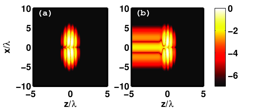
Figure 1: Logarithm of the square transverse magnetic field $\log_{10}\left((B_{y}/B_{0})^{2}\right)$ in the $y=0$ plane resulting from an ultrashort, linearly polarized, (a) sine- and (b) cosine-phased Gaussian potential. The pulse duration is $c\tau=0.5\,\lambda$ and focal spot width $\sigma=2\,\lambda$.

To get a realistic finite energy pulse, our choice of the transverse vector potential is restricted by Eq. (1). This is a fundamental difference to the 1D case, where such a restriction on the wave form does not exist. Before the consequences of this restriction are discussed in detail, let us introduce the second potential $\bf{\Psi}$, which enables us to describe a reasonable set of realistic pulse structures in a more convenient way:

$$\mathbf{A}=\nabla\times{\bf\Psi}$$ (2)

Of course, each component of $\bf\Psi$ has to satisfy the wave equation $\Delta\Psi_{i}-\frac{1}{c^{2}}\partial_{t}^{2}\Psi_{i}=0$. Then, the wave equation for $\mathbf{A}$ and the Coulomb gauge readily follow from Eq. (2) and there are no restrictions like (1) on the choice of the second potential components.

For a large class of laser pulses, it is convenient to choose $\hat{\mathbf{e}}_{z}\cdot{\bf\Psi}=0$. Then Eq. (2) becomes $A_{z}=-\nabla_{\perp}\cdot\left(\hat{\mathbf{e}}_{z}\times{\bf\Psi}\right)$ and $\mathbf{A}_{\perp}=\hat{\mathbf{e}}_{z}\times\partial_{z}{\bf\Psi}$. In the near-monochromatic case $\partial_{z}\sim-i\omega/c$ we get $\hat{\mathbf{e}}_{z}\times{\bf\Psi}\approx ic\mathbf{A}_{\perp}/\omega$, hence in the long pulse limit the transverse second potential (TSP) $\hat{\mathbf{e}}_{z}\times{\bf{\Psi}}$ is, except for a constant factor, identical with the transverse components of the vector potential.

Let us point out that each electromagnetic pulse in vacuum can be represented by the TSP. This is easily seen, since the second potential can be obtained by taking the integral $\hat{\mathbf{e}}_{z}\times\bf{\Psi}=\int_{z}^{\infty}\mathbf{A}_{\perp}dz^{\prime}$ from an arbitrary vector potential in Coulomb gauge. To make the representation unique, we require the condition $|{\bf{\Psi}}|\rightarrow 0$ for $|\mathbf{r}|\rightarrow\infty$ in the half-space $x>0$, so that $\bf{\Psi}_{\perp}$ is unambiguously given by the just mentioned integral. Then, for a vast class of laser pulses including all linearly, circularly and radially polarized modes, ${\bf{\Psi}}$ will vanish at infinity in all directions. To understand this, we write the integral condition (1) in terms of the TSP:

$$\nabla_{\perp}\cdot\left(\hat{\mathbf{e}}_{z}\times\left.\Psi\right|_{z=-\infty}\right)=0$$ (3)

In general, it possesses non-trivial solutions, corresponding to structures, where the fields produced by ${\bf{\Psi}}$ at $z\rightarrow-\infty$ vanish, but ${\bf{\Psi}}$ itself does not. However, we look at important special cases. For linear polarization ($\Psi_{x}=0$), Eq. (3) has obviously none but the trivial solution. Thus, all finite energy, linearly polarized pulses can be represented by a localized TSP. The same is true for circular polarization, which we define by $\Psi_{y}=i\Psi_{x}$, and the components are assumed to be analytical functions. Eq. (3) then only has solutions of the type $\Psi(x+iy)$, so there is no non-trivial solution that fulfills the boundary condition. Another interesting structure is the radially polarized pulse ($\hat{\mathbf{e}}_{z}\times\mathbf{\Psi}=f(r_{\perp},z,t)\mathbf{r}_{\perp}$), and again there is no non-trivial finite energy solution to (3) obeying its symmetry.

Summarizing, for each realistic linearly, circularly or radially polarized pulse, the condition $\hat{\mathbf{e}}_{z}\times\left.\bf{\Psi}\right|_{z=-\infty}=\int_{-\infty}^{\infty}\mathbf{A}_{\perp}dz\overset{!}{=}0$ on the transverse vector potential must be fulfilled. Commonly used analytical wave packet solutions strictly fulfill this condition only for a certain choice of the CEP. Take, for instance, a pulse with a Gaussian longitudinal profile, $A_{y}(x=0,\,y=0,\,z,\,t=0)=a_{0}\exp\left[-(z/c\tau)^{2}\right]\cos(2\pi z/\lambda)$, then $\left|\Psi_{y}(z=-\infty)\right|/(a_{0}\lambda)=\pi^{-1/2}\overline{\tau}\,\exp\left(-\overline{\tau}^{2}\right)\neq 0$, meaning that some field components would extend to infinity as in Fig. 1b. Unlike the cosine-phased Gaussian, the sine-phased potential may in principle be assigned to $A_{y}$, as the integral vanishes here (see also Fig. 1a). Assigning an exact Gaussian profile to the transverse electric field instead does not help. Indeed, by calculating the second potential of such a pulse it can be proven that this structure does not exist for any phase.

Other than for linearly, circularly or radially polarized pulses, for the azimuthally polarized pulse $\hat{\mathbf{e}}_{z}\times\mathbf{\Psi}=f(r_{\perp},z,t)\hat{\mathbf{e}}_{\varphi}$ the TSP representation not have to vanish as $z\rightarrow-\infty$. Notice that this pulse does not produce any longitudinal field at all. Anyway, it can neatly be represented by the longitudinal component $\hat{\mathbf{e}}_{z}\cdot{\bf\Psi}$ instead of the transverse components of the second potential.

III Scalar Wave Equation

Now we come to the solution of the scalar wave equation on $\bf\Psi$. The Fourier transform in time and the transverse directions yields $\partial_{z}^{2}\tilde{\Psi}=-((\omega/c)^{2}-k_{\perp}^{2})\tilde{\Psi}$, with the solution

$$\tilde{\Psi}(x,\mathbf{k}_{\perp},\omega)=\left.\tilde{\Psi}\right|_{z=0}\exp\left(-iz\sqrt{\left(\frac{\omega}{c}\right)^{2}-k_{\perp}^{2}}\right)$$ (4)

Next, the focal spot profile $\tilde{\Psi}(z=0)$ has to be chosen in a physically reasonable way. Besides the very common linearly polarized Gaussian mode $\textrm{TEM}_{00}$, we also treat the very interesting radially polarised Hermite-Gaussian mode $\textrm{TM}_{01}$. Further we will tackle the 2D solutions, which differ in some factors from the 3D ones. Knowing the scalar solution for the $\textrm{TEM}_{00}$ mode, we can easily construct circularly polarized Gaussian pulses by setting $\Psi_{y}=i\Psi_{x}$, and moreover azimuthally polarized pulses by assigning the same term to the longitudinal component $\hat{\mathbf{e}}_{z}\cdot\bf{\Psi}$ of the second potential.

Let $\psi(t)$ be the pulse time dependence at the center of the focal spot and $\tilde{\psi}(\omega)$ its Fourier transform. The focal spot size may depend on the frequency:

$$\left(\hat{\mathbf{e}}_{z}\times\left.\tilde{\bf{\Psi}}\right|_{z=0}\right)=\tilde{\psi}(\omega)\,\exp\left[-\left(\frac{r_{\perp}}{\sigma\left(\omega\right)}\right)^{2}\right]\begin{cases}\mathbf{r}_{\perp}&\textrm{TM}_{01}\\ \hat{\mathbf{e}}_{x}&\textrm{TEM}_{00}\end{cases}$$ (5)

Now, the transverse direction Fourier transform of (5) is inserted into the solution of the wave equation (4). Since we consider pulses propagating mainly in one direction ($c^{2}k_{\perp}^{2}\ll\omega^{2}$), we expand the square root in a Taylor series and neglect fourth order terms: $\sqrt{\left(\omega/c\right)^{2}-k_{\perp}^{2}}\approx\omega/c-ck_{\perp}^{2}/(2\omega)$, performing the paraxial approximation. If now $\sigma\propto 1/\sqrt{\omega}$ is assumed, so that the Rayleigh length $z_{Rl}=\omega\sigma^{2}/2c$ is constant for all frequencies, we are able to carry out the inverse Fourier transform analytically and obtain the solution

$$\hat{\mathbf{e}}_{z}\times\mathbf{\Psi}\left(\mathbf{r},t\right)=\left(\frac{z_{Rl}}{q}\right)^{g}\,\psi\left(t-\frac{z}{c}-\frac{r_{\perp}^{2}}{2cq}\right)\begin{cases}\mathbf{r}_{\perp}&\textrm{TM}_{01}\\ \hat{\mathbf{e}}_{x}&\textrm{TEM}_{00}\end{cases}$$ (6)

Here $g=1$ for a linear ($g=0.5$ in 2D) and $g=2$ for a RP ($g=1.5$ in 2D) laser and $q=z+iz_{Rl}$ is the confocal parameter. $\psi$ is a complex representation of the time dependence of the pulse. Note, that since $t^{\prime}=t-z/c-r_{\perp}^{2}/2cq$, it is generally a complex number. Choosing naively $\psi(t^{\prime})=\exp\left(-t^{\prime 2}/\tau^{2}+i(\omega_{0}t^{\prime}+\phi)\right)$ yields a solution diverging for big $r_{\perp}$ as $\mathcal{O}(\exp(r_{\perp}^{4}))$. Instead the analytic signal (Bracewell, ) should be used, as suggested by Porras (porras, ). The analytic signal is the complex representation of a real signal without negative frequency components. The analytic signal representation of the Gaussian pulse $g(t^{\prime})=\exp(-t^{\prime 2}/\tau^{2})\cos(\omega_{0}t+\phi)$ is calculated to be

$$\psi\left(t^{\prime}\right)=\psi_{0}\frac{e^{-\overline{\tau}^{2}}}{2}\left(e^{i\phi}w\left(\frac{t^{\prime}}{\tau}-i\overline{\tau}\right)+e^{-i\phi}w\left(\frac{t^{\prime}}{\tau}+i\overline{\tau}\right)\right)$$ (7)

wherein $\overline{\tau}=\omega_{0}t/2$ and $w\left(z\right)=\textrm{exp}(-z^{2})\textrm{erfc}(-iz)$ is the complex error (or Faddeeva) function (Abramowitz, ). The analytic signal of the Gaussian pulse was also calculated in (porras, ), but Eq. (27) from (porras, ) disagrees with (7) for $\textrm{Im}(t^{\prime})\neq 0$. Analytical and numerical tests show, that (7) is the correct solution. To illustrate the meaning of (7) and its difference to the naive choice $\psi(t^{\prime})=\exp\left(-t^{\prime 2}/\tau^{2}+i(\omega_{0}t^{\prime}+\phi)\right)$, consider Fig. 2. In the region near the optical axis, $\textrm{Im}(t^{\prime})$ is small and the solutions agree quite well. However, for bigger $r_{\perp}$ the naive solution (b) diverges, while the analytic signal shows a proper beam-like behaviour and vanishes.

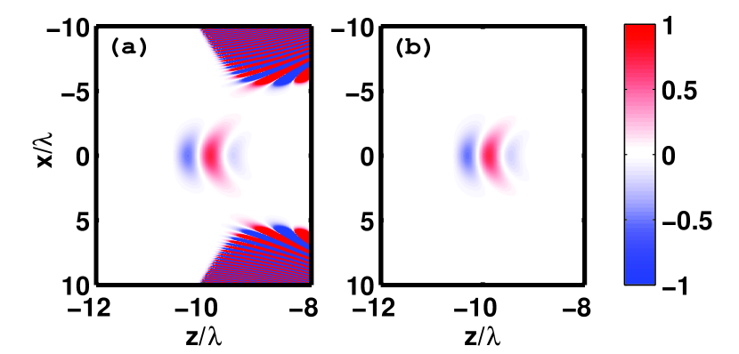
Figure 2: Direct comparison of a two dimensional cut through the complete short-pulse solution (6) using (a) the “naive” choice $\psi(t^{\prime})=\exp\left(-t^{\prime 2}/\tau^{2}+i(\omega_{0}t^{\prime}+\phi)\right)$ and (b) the analytic signal Eq. (7). Pulse parameters are: $c\tau=0.5\,\lambda$, $\sigma=2\,\lambda$, $ct=-10\,\lambda$ (before focus)

IV Numerical Testing

The equations (2), (6) and (7) together form the key to accurate analytical and numerical representation of ultrashort few- and even single-cycle electromagnetic pulses. One important application of them is the use in numerical simulations and we will conclude this paper by showing their superiority to more conventional representations for this application, thereby checking the correctness and the accuracy of the analytical results obtained so far.

We use the particle in cell (PIC) code VLPL (vlpl, ). To begin with, the fields are initialised inside the VLPL simulation grid. Then they are propagated using a standard algorithm on the Yee-mesh. Finally, it is verified if the numerically propagated pulse still agrees with the analytical term, overall or in some key parameters, and furthermore, if unphysical static fields remain at the place, where the pulse was initialized.

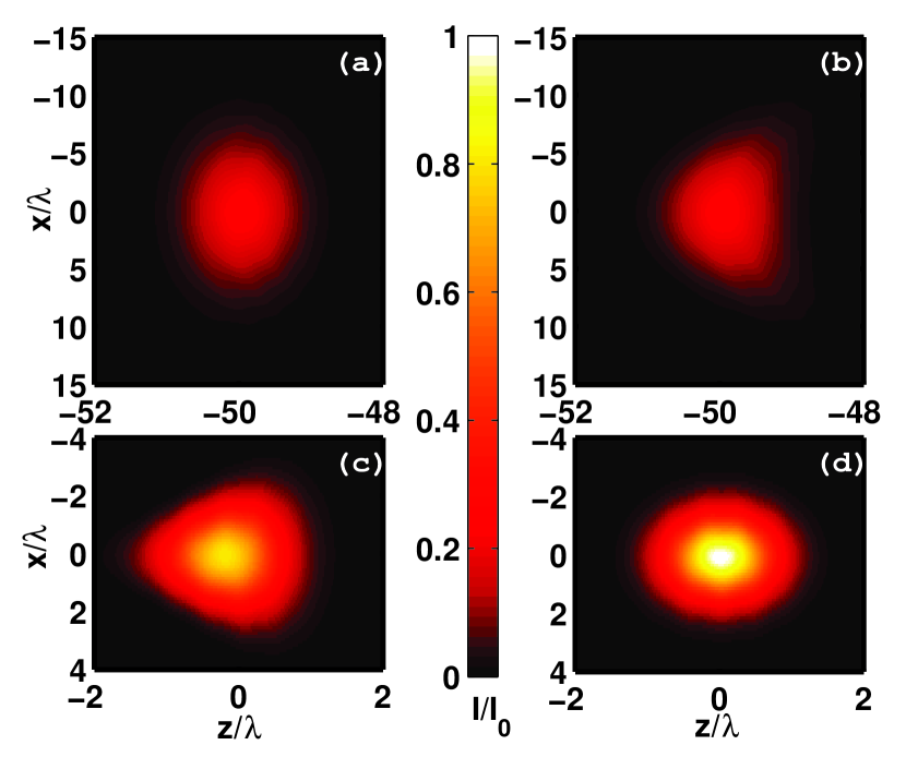
Figure 3: Focusing properties of different approximations of the wave equation, evaluated in a 2D version of the PIC code VLPL. (a) and (b) show the intensity distribution as it is initialised inside the code and (c) and (d) show the propagated solution at the focal spot. (a) and (c) use the CW paraxial solution multiplied with a temporal profile, (b) and (d) the correct short pulse solution. The circularly polarized laser pulses are Gaussian both in space and time with duration $c\tau=\lambda$ and width $\sigma=2\lambda$.

First we check the correctness of Eqs. (6) and (7), proving their superiority to a conventional representation often used for numerical simulations. The “conventional”, or separable form is a simple product of a monochromatic, transversely Gaussian beam with a Gaussian temporal profile. Circularly polarized pulses are used, so that the shape can well be seen in the intensity plots, with a duration of $c\tau=\lambda$ and a focal spot width of $\sigma=2\lambda$. The pulses are focused over a distance of $50\lambda$ inside the simulation. In Fig. 3 the initial condition and the numerically propagated solution at the focal spot are shown. While the product approximation shows strong asymmetric deformation in the focus and the focal field does not reach its specified value of $a_{0}=1$, the proper short pulse solution is nearly perfectly symmetric in the focus and reaches the desired maximum. The presented solution Eqs. (6) and (7) is clearly superior to the simple product approach.

Now we come to the second potential representation. The alternative to its use is to assign arbitrary wave equation solutions to the transverse components of the vector potential and then make some kind of approximation for the longitudinal part. The simplest possibility is to fully neglect the longitudinal field component, but for strongly focused pulses a somewhat more reasonable approximation can be reached by choosing $A_{z}=(c/i\omega_{0})\nabla_{\perp}\cdot\mathbf{A}_{\perp}$, what we will call the quasi-monochromatic approximation, because it relies on $\partial_{z}\sim-i\omega_{0}/c$. Using one of these approximations, the initial pulse structure has finite energy, and because of the energy conserving property of the field propagator algorithm, the pulse will be forced to self-organize into a consistent structure of finite extension. While this happens, “virtual charges” are left behind, unphysical static fields, which may make the concerned regions in the simulation domain unusable for further computations. We want to see, if this problem can be cured by the use of the second potential representation.

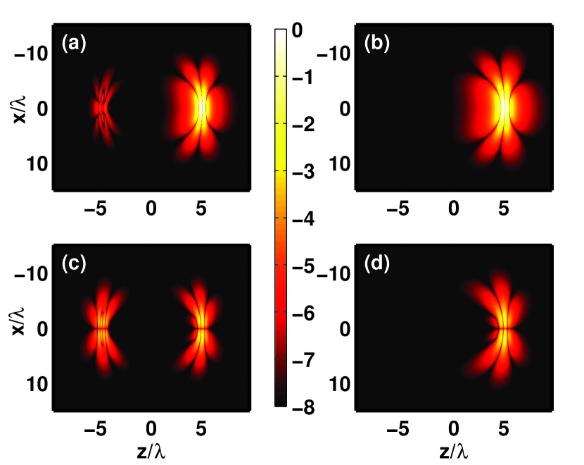
Figure 4: Logarithm of the transverse ((a) and (b)) and longitudinal ((c) and (d)) square electric field $\log_{10}\left((E_{i}/E_{0})^{2}\right),\;i\in\{x,z\}$ after a propagation time $ct=10\,\lambda$. (a) and (c) depict the conventional, (b) and (d) the TSP Gaussian. Pulse parameters are $c\tau=0.3\,\lambda$ and $z_{Rl}=4\pi^{2}\,\lambda$. For the second potential, a corrected frequency $\omega_{0}^{\prime}=\omega_{0}-\sqrt{2}/\tau$ was used to take account for the frequency shift caused by the additional derivative.

When employing the second potential representation for an ultrashort pulse, the additional derivative will slightly alter the pulse shape. As shown before, this is inevitable, since a Gaussian shaped linearly polarized vector potential can exist as an independent structure in vacuum only if it is sine-phased. To make the TSP represented pulse comparable to the conventional one, it is necessary to take care for the frequency shift caused by the $z$-derivative, which can be estimated as $\omega_{\textrm{eff}}=\omega_{0}+\sqrt{2}/\tau$.

Fig. 4 shows the pulses after a short propagation distance in the PIC simulation box. Firstly one observes that, despite of the very short duration, the moving pulse structures (right half of the images) appear very similar in the conventional and the TSP version. Secondly one notices, that the conventional pulse leaves behind a significant amount of virtual charge fields in the initialisation region (left half of the images), having both a longitudinal and a transverse component. This undesired phenomenon can neatly be suppressed by the use of the second potential, seen in the figure.

The last test we want to present in this paper concerns the longitudinal field component on the optical axis of a radially polarized pulse, which is of particular interest for vacuum electron acceleration (salamin RP, ; anupam, ; canada, ). The pulse length used was $c\tau=0.5\lambda$, and the focal spot size $\sigma=2\lambda$. Again, the conventional approach corresponds to a near-monochromatic approximation $A_{x}=i\nabla_{\perp}\cdot\mathbf{A}_{\perp}/\omega$, so as to generate a finite pulse structure from the given transverse field components. The phase $\phi$ in Eq. (7) was chosen as $\phi=0$ for the second potential representation and as $\phi=0.5\,\pi$ for the conventional representation, so that the pulses are actually comparable. Initially, the longitudinal field nearly agrees for both representations, since the first term of Eq. (7), which is the dominating one, is the same in both cases.

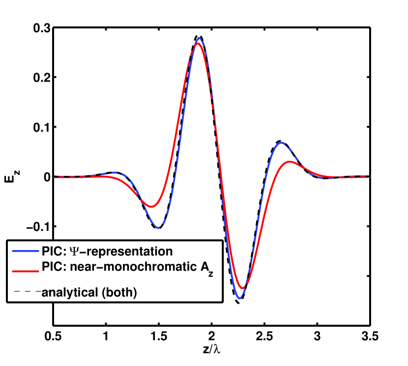
Figure 5: The longitudinal pulse field in PIC at the time $c(t-t_{0})=4\lambda$ after initialization, compared to the analytic solution. Once the TSP was used for initialization (blue line) and once the near-monochromatic approximation for $A_{z}$. The differences in the analytical representations are too small to be seen in the diagram, so that both are represented by one curve (dashed black line). Pulse parameters are: $c\tau=0.5\lambda$, $\sigma=2\lambda$,

In figure 5 we present the longitudinal field of the pulse after it has left its “virtual charges” behind. The fields initialized using the conventional representation already differ significantly from the analytical description, whereas the TSP represented fields agree almost perfectly. This will be crucial e.g. when PIC simulations are to be compared with other analytical or semi-numerical calculations, where the field is inserted analytically and is not self-consistently propagated. Without an exact and reliable pulse representation, such a comparison is hardly possible.

V Conclusion

In this paper we have given a comprehensive guide to the mathematical representation of ultrashort, Gaussian and related, electromagnetic pulses. The wave equation for an ultrashort Gaussian pulse has been solved in paraxial approximation. Further it has been shown, that the vectorial character of light has a stringent influence on its field structure for ultrashort pulses. To pay regard to this, ultrashort pulses should be represented by their second potential, using the transverse components for linear, circular or radial polarization and the longitudinal component for azimuthal polarization. Numerical tests proove that the solutions flawlessly work in the regime of ultrashort, moderately strong ($\sigma\gtrsim\lambda$) focused pulses.

References

- (1) G. A. Mourou, et al. Plasma Phys. Control. Fusion 49 B667-B675 (2007).
- (2) L. Xu, Ch. Spielmann, A. Poppe, T. Brabec, F. Krausz, and T. W. Hänsch, Opt. Lett. 21(24), 2008 (1996).
- (3) David J. Jones, et al. Science 288, 635 (2000).
- (4) G. G. Paulus, et al. Nature (London) 414, 182-184 (2001).
- (5) P. B. Corkum, F. Krausz, Nature Phys. 3, 381 (2007)
- (6) Y. I. Salamin and C. H. Keitel, Phys. Rev. Lett. 88(9), 095005 (2002).
- (7) Y. I. Salamin, Phys. Rev. A 73, 043402 (2006).
- (8) C. Varin, M. Piche, and M. A. Porras, Phys. Rev. E 71, 026603 (2005).
- (9) A. Karmakar and A. Pukhov, Laser and Particle Beams 25, 371 (2007).
- (10) N. M. Naumova, J. A. Nees, B. Hou, G. A. Mourou and I. V. Sokolov, Opt. Lett. 29(7), 778 (2004).
- (11) T. Baeva, S. Gordienko and A. Pukhov, Phys. Rev. E 74, 065401(R) (2006).
- (12) G. D. Tsakiris, K. Eidmann, J. Meyer-ter-Vehn, and F. Krausz, New J. Phys. 8, 19 (2006).
- (13) A. Pukhov, Nature Physics, 2, 439 (2006).
- (14) M. Lax, W. H. Louissell, W. B. McKnight, Phys. Rev. A 11(4), 1365 (1975).
- (15) M. A. Porras, Phys. Rev. E 58(1), 1086 (1998).
- (16) M. A. Porras, Phys. Rev. E 65, 026606 (2002).
- (17) R. Bracewell, The Fourier Transform and Its Applications, (McGraw-Hill, 2nd ed. 1986).
- (18) S. Quabis, R. Dorn, M. Eberler, O. Glöckl, G. Leuchs, Appl. Phys. B 72, 109 (2001).
- (19) R. Dorn, S. Quabis, and G. Leuchs, Phys. Rev. Lett. 91(23), 233901 (2003).
- (20) M. Abramowitz, I. A. Stegun, Handbook of Mathematical Functions with Formulas, Graphs, and Mathematical Tables, (New York, Dover 1972).
- (21) A. Pukhov, J. Plasma Phys. 61, 425 (1999).