A high order purely frequency-based harmonic balance formulation for continuation of periodic solutions

Abstract

Combinig the harmonic balance method (HBM) and a continuation method is a well-known technique to follow the periodic solutions of dynamical systems when a control parameter is varied. However, since deriving the algebraic system containing the Fourier coefficients can be a highly cumbersome procedure, the classical HBM is often limited to polynomial (quadratic and cubic) nonlinearities and/or a few harmonics. Several variations on the classical HBM, such as the incremental HBM or the alternating frequency/time domain HBM, have been presented in the literature to overcome this shortcoming. Here, we present an alternative approach that can be applied to a very large class of dynamical systems (autonomous or forced) with smooth equations. The main idea is to systematically recast the dynamical system in quadratic polynomial form before applying the HBM. Once the equations have been rendered quadratic, it becomes obvious to derive the algebraic system and solve it by the so-called ANM continuation technique. Several classical examples are presented to illustrate the use of this numerical approach.

1 Introduction

In the field of engineering, especially when dealing with nonlinear vibrations, it is often required to compute the periodic solutions of a system of nonlinear differential equations ([1, 2]). In the following, we focus on numerical methods to find periodic solutions. They are usually subdivided into two main groups : those relying on the time-domain formulation and those relying on the frequency-domain formulation. The first group consists of methods where a time integration algorithm, which is generally limited to a single period, is used to transform the original differential system into a system of algebraic equations, which are then solved by continuation. With these methods, the unknowns in the algebraic system are the values of the original unknown variables at grid points along the periodic orbit. The classical shooting technique ([3, 4]) and the orthogonal collocation methods used in AUTO ([5, 7]) belong to this group. The second group corresponds to the so-called harmonic balance method where the unknown variables are decomposed into truncated Fourier series. In this case, the unknowns in the final algebraic system, which is obtained by balancing the harmonics featuring in the differential equations, are simply the Fourier coefficients of the original unknowns. Methods of both kinds are widely used in many applications and research is still required to improve them. In practical terms, the choice between the time-domain or the frequency-domain approach depends mainly on whether the periodic solution can be decomposed with a few Fourier components. The method chosen to deal with a given problem can therefore depend on the operating point.

In this paper, we focus on the harmonic balance method (HBM) and some of its variations, which are briefly recalled here. Although the name "harmonic balance" seems to have first appeared in 1936 ([8]), this method has been widely used only since the sixties, and especially for electrical and mechanical engineering purposes. Forced vibrations were first studied ([9]), and self-sustained oscillations a decade later ([10]). The study by Nakhla & Vlach ([11]) is often said to be a milestone in the modern formulation of HBM. The classical HBM is simple in its principle, but it can be cumbersome or even impracticable, as stated by Peng et al. ([12]) when the system contains complex nonlinearities and when a large number of harmonics is required, ie, more than 5 or 10. The first problem which arises is how to derive the algebraic system for the Fourier coefficients and the second problem is how to solve this strongly nonlinear system efficiently. To overcome these shortcomings, many variations on the basic HBM have been proposed in the literature. Here, we will simply give an overall picture of incremental harmonic balance (IHB) and alternating frequency/time domain harmonic balance (AFT) method. With the IHB method ([13]), the incremental-iterative method used for the continuation is closely combined with the harmonic principle, so as to be able to apply the HB principle to the incremental linear problem instead of the nonlinear original system. Nonlinearity of all kinds can be treated using this technique [14, 15]. In the AFT variant, the harmonic balance of the Fourier coefficients is not explicitly performed. At each increment (or iteration) in the continuation procedure, the unknowns are transferred to the time domain (using the inverse Fast Fourier Transform,which is denoted IFFT below), so as be able to use the original system of equations. The nonlinear responses are then transferred back to the frequency domain using the Fast Fourier Transform, (denoted FFT below). The use of FFT/IFFT procedures seems to have started in [16]. This technique has been used, for instance, to analyse nonlinear vibrations in mechanical systems with contact and dry friction [17]. Since the pioneering work on IHB and AFT, many variations have been proposed to extend the applications, as well as to decrease the computational cost (see [18] or [19] for some recent examples).

An alternative strategy is proposed here for applying the classical HBM with a large number of harmonics, without avoiding explicit balancing. The idea is to apply a transformation to the original system of differential equations before applying the HBM. The aim of this procedure is to transform the non-linearities present in the original system into purely polynomial quadratic terms. The classical HBM procedure can then be easily applied. This transformation might seem to be a limitation of the method, since not every system can be recast in polynomial quadratic form. However, it will be shown in this paper that a very large class of systems with smooth equations can indeed be recast in quadratic form by making a few algebraic manipulations and a a few additions of equations and auxiliary variables. The idea of using a quadratic formulation to simplify the (Fourier) series expansion was inspired by another numerical method, the so-called Asymptotic Numerical Method (ANM) ([21, 22]) which was presented for the first time in 1990 ([20]). ANM is a continuation technique ([23]) involving high order powers series expansion of the branches of solutions. For reasons that will be given later on, this ANM continuation is the ideal means of solving the algebraic system resulting from the HB method proposed here.

The paper is organised as follows: details of the transformation into a polynomial quadratic form, the application of the HBM method and the principle of continuation are given in section 2 in the cases of autonomous systems. Three simple examples are given as an illustration. Section 3 is devoted to periodically forced systems, and two further examples are presented. Section 4 gives the results of all the examples and ends with some concluding comments and perspectives.

2 Presentation of the method for obtaining periodic solutions of autonomous systems

Let us consider an autonomous system of differential equations

$$\dot{Y}=f(Y,\lambda)$$ (1)

where $Y$ is a vector of unknowns, $f$ a smooth nonlinear vector valued function and $\lambda$ a real parameter. The dot stands for the derivative with respect to time $t$. We assume that this system has branches of periodic solutions when $\lambda$ varies, and we want to find and follow them by applying the harmonic balance method and a continuation procedure (path following technique). The important case of a forced (non-autonomous) system will be dealt with separately in section 3.

2.1 The harmonic balance principle

As recalled in the Introduction, the HBM consists basically in decomposing $Y(t)$ into a truncated Fourier series :

$$Y(t)=Y_{0}+\sum_{k=1}^{H}Y_{c,k}\cos(k\omega t)+\sum_{k=1}^{H}Y_{s,k}\sin(k\omega t)$$ (2)

This ansatz is put into Eq. (1) and $f(Y,\lambda)$ is expanded into Fourier series. By balancing the first $2H+1$ harmonic terms, one obtains an algebraic system with $2H+1$ vector equations for the $2H+1$ vector unknowns $Y_{i}$, the unknown pulsation $\omega$, and the parameter $\lambda$. Adding a phase condition ([3]) yields a system with $N$ equations and $N+1$ variables. The branches of solutions of this algebraic system are then followed using a continuation technique. This procedure provides only approximate periodic solutions, since in the expansion of Eq. (1), all the harmonic terms greater than $H$ remain unbalanced. However, if the number of harmonics $H$ is large enough, accurate solutions can be obtained.

The most crucial point is the expansion of the vector $f(Y,\lambda)$ into Fourier series. This can be quite a straighforward procedure if $f(Y,\lambda)$ is a polynomial of degree two or three, and if the number of harmonics $H$ is sufficiently small. In this case, the expansion can be carried out by hand. But in the most general situation, where $f(Y,\lambda)$ shows nonlinearities of any kinds, this computation can be very cumbersome, even with the help of a symbolic software program. The only alternative is then to use numerical procedures to estimate the Fourier series of $f(Y,\lambda)$, by performing iterative FFT/IFFT steps, for example. This drawback was the starting-point in the developpment of many variants of the HBM as mentioned in the Introduction.

2.2 A key point: the quadratic recast

The main aim of this paper is to present a simple but powerful procedure that overcomes the drawback mentioned above. The idea is to recast the original system (1) into a new system where the nonlinearities are at most quadratic polynomials . The application of the harmonic balance method subsequently becomes quite straighforward. This new quadratic system, which will be written as follows

$$m(\dot{Z})=c+l(Z)+q(Z,Z)$$ (3)

can contain both differential and algebraic equations. $N_{e}$ is taken to denote the number of equations. The unknown vector $Z$ (size $N_{e}$) contains the original components of the vector $Y$ and some new variables which are added to get the quadratic form. The right hand side of Eq. (3) is written as follows: $c$ is a constant vector with respect to the unknown $Z$, $l(.)$ is a linear vector valued operator with respect to the vector entry, and $q(.,.)$ is a quadratic vector valued operator, which is linear with respect to both entries. At this stage, the three vectors $c$, $l(.)$ and $q(.,.)$ may depend on the real parameter $\lambda$. However, it is preferable for the quadratic operator $q(.,.)$ not to depend on $\lambda$, which may require introducting a new variable in $Z$ (see example 1 below). on the left hand side, $m(.)$ is a linear vector valued operator with respect to the vector entry. The algebraic equations correspond to zero values of $m(.)$.

Since the nonlinearities are quadratic, the HBM can obviously be easily and systematically applied on Eq. (3), even with a large number of harmonics. The question is now: can any system be easily put into the form of Eq. (3) ? As we will see, the answer is yes, for a very large class of nonlinear systems.

The idea of recasting a nonlinear system into a new one with a quadratic polynomial nonlinearity is frequently used when considering the so-called ANM continuation method, which consists in computing power series expansion of solution branches, see ([21, 22, 23, 24]) for the basic algorithms and ([25, 26, 27]) for some applications in mechanics. The quadratic recast gives a very simple and systematic algebra for the series determination, even with high orders of truncature. Similar benefits are obtained with the Fourier series expansions.

It is now worth illustrating this main idea by giving some elementary examples where the recast from Eq. (1) to Eq. (3) will be performed explicitely. We will deal first with the classical Van der Pol oscillator, the Rössler system and a model for clarinet-like musical instruments. Other examples, with nonlinearities of others kinds such as rational fraction, will be given later on.

Example 1: The Van der Pol oscillator. We take the following second order autonomous system, known as the Van der Pol oscillator, where the parameter $\lambda$ governs the amplitude of the nonlinear damping term.

$$\ddot{u}-\lambda(1-u^{2})\;\dot{u}+u=0$$ (4)

This equation can be classically recast into first order system ( as Eq. (1)) by introducing the velocity $v(t)=\dot{u}(t)$ as a new unknown. We obtain

$$\begin{array}[]{ccc}\dot{u}&=&v\\ \dot{v}&=&\lambda(1-u^{2})\;v-u\end{array}$$ (5)

If we now introduce the auxiliary variables $w(t)=1-u^{2}(t)$ and $r(t)=v(t)w(t)$, the system can be written in the form of Eq. (3) with $Z=[u,v,w,r]^{t}$. The various terms are arranged below so that it will be clear to the readers how the different functions $m$, $c$, $l$ and $q$ are formed.

$$\begin{array}[]{ccccc}\dot{u}&=&0&+v&\\ \dot{v}&=&0&-u+\lambda r&\\ 0&=&1&-w&-u^{2}\\ \underbrace{0}_{m(\dot{Z})}&=&\underbrace{\quad\ 0\quad}_{c}&\underbrace{\quad\quad+r\quad\quad}_{l(Z,\lambda)}&\underbrace{\quad-vw\quad}_{q(Z,Z)}\\ \end{array}$$ (6)

We finally obtain two first order differential equations and two algebraic equations with quadratic polynomial nonlinearities. Only the operator $l$ depends here on $\lambda$.

Example 2: The Rössler system. We take the following first order autonomous system of three equations known as the Rössler system.

$$\begin{array}[]{lcl}\dot{x}&=&-y-z\\ \dot{y}&=&x+ay\\ \dot{z}&=&b+z(x-\lambda)\end{array}$$ (7)

where $x$, $y$, $z$ are functions of time and $a$, $b$, $c$ are float parameters. This system can be written in the form of Eq. (3) without any auxiliary variables (i.e. $Z=[x,y,z]^{t}$):

$$\begin{array}[]{ccccc}\dot{x}&=&0&-y-z&\\ \dot{y}&=&0&+x+ay&\\ \underbrace{\dot{z}}_{m(\dot{Z})}&=&\underbrace{\quad b\quad}_{c}&\underbrace{\quad\quad-\lambda z\quad\quad}_{l(Z,\lambda)}&\underbrace{\quad+zx\quad}_{q(Z,Z)}\\ \end{array}$$ (8)

Here again, only the operator $l$ depends on $\lambda$. This example will be used here to show that the approach presented in this paper can be used to find period-doubling and bifurcations with period 4.

Example 3: A model for clarinet-like musical instruments. In the case of small amplitude oscillations, a simple model for reed instruments (clarinet, saxophone, etc) can be written using a modal formulation (see [28]):

$$\begin{array}[]{l}\ddot{x}+q_{r}\omega_{r}\dot{x}+\omega_{r}^{2}x=\omega_{r}^{2}p\\ \ddot{p}_{n}+2\alpha_{n}c\,\dot{p}_{n}+\omega_{n}^{2}p_{n}=\frac{2c}{l}\,\dot{u}\qquad\forall n\in[1\dots N]\\ u=\zeta(1-\lambda+x)\sqrt{\lambda-p}\\ p=\sum_{n=1}^{N}p_{n}\end{array}$$ (9)

where the unknowns $x$, $p_{n=1..N}$, $p$, $u$ are functions of time and $q_{r}$, $\omega_{r}$, $\alpha_{n}$, $\omega_{n}$, $c$, $l$, $\zeta$ are given parameters describing either the physics or the player’s action. $N$ is the number of acoustic modes. $\lambda$ stands here for the blowing pressure.

It is worth noting that even if this system contains a square root, it can be recast in the form of Eq. (3): if we introduce the auxiliary variables $y=\dot{x}$, $z_{n}=\dot{p}_{n}$ and $v=\sqrt{\lambda-p}$, system (9) can be rewritten, with $Z=[x,y,p_{1},\dots,p_{N},z_{1}\dots z_{N},u,v]^{t}$ as follows:

$$\begin{array}[]{cccccc}\dot{x}&=&0&+y&\\ \dot{y}&=&0&+\omega_{r}^{2}p-q_{r}\omega_{r}y-\omega_{r}^{2}x&\\ \dot{p}_{n}&=&0&+z_{n}&&\quad\forall n\in[1\dots N]\\ \dot{z}_{n}-\frac{2c}{l}\dot{u}&=&0&-2\alpha_{n}c\,z_{n}-\omega_{n}^{2}p_{n}&&\quad\forall n\in[1\dots N]\\ 0&=&0&-u+\zeta(1-\lambda)v&+\zeta xv\\ 0&=&0&-p+p_{1}+\dots+p_{N}&\\ \underbrace{\qquad 0\qquad}_{m(\dot{Z})}&=&\underbrace{\quad\lambda\quad}_{c(\lambda)}&\underbrace{\quad\quad\quad\quad-p\quad\quad\quad\quad}_{l(Z,\lambda)}&\underbrace{\quad-v^{2}\quad}_{q(Z,Z)}\\ \end{array}$$ (10)

Here, the linear term $l$, but also the constant term $c$, are functions of $\lambda$.

2.3 The harmonic balance method applied to a quadratic system

In this section, the harmonic balance method is applied to the system (3). The unknown (column) vector $Z$ is decomposed into Fourier series with $H$ harmonics:

$$Z(t)=Z_{0}+\sum_{k=1}^{H}Z_{c,k}\cos(k\omega t)+\sum_{k=1}^{H}Z_{s,k}\sin(k\omega t)$$ (11)

The components of the Fourier series are collected into a large (column) vector $U$, with size $(2H+1)\times N_{e}$, where $N_{e}$ is the number of equations in (3).

$$U=[Z_{0}^{t},Z_{c,1}^{t},Z_{s,1}^{t},Z_{c,2}^{t},Z_{s,2}^{t},\dots,Z_{c,H}^{t},Z_{s,H}^{t}]^{t}$$ (12)

By introducing the expansion (11) into the set of Eqs. (3), collecting the terms of the same harmonic index, and neglecting the higher order harmonics, one obtains a large system of $(2H+1)\times N_{e}$ equations for the unknown vector $U$,

$$\omega M(U)=C+L(U)+Q(U,U)$$ (13)

The new operators $M(.)$, $C$, $L(.)$, and $Q(.,.)$ that apply to $U$ depend only on the operators $m(.)$, $c$, $l(.)$ and $q(.,.)$ of Eq. (3) and on the number of harmonics H. The explicit formulas have been given in annex 1 for a sake of brevity. It should be noted that these expressions for $M(.)$, $L(.)$ and $Q(.,.)$ are the same in all the examples presented. The change from one particular system to another only involves the operators $m(.)$, $l(.)$ and $q(.,.)$.

The final system (13) contains $(2H+1)\times N_{e}$ equations for the $(2H+1)\times N_{e}$ unknowns $U$ plus the angular frequency $\omega$ and the continuation parameter $\lambda$. Since the original system is autonomous, a phase condition has to be added to Eq. (13) to define a unique orbit. Indeed, the time $t$ does not appear in Eq. (3) and if $U(t)$ is a solution of Eq. (13) then $U(t+\tau)$ is also a solution, for any $\tau$. We refer here to textbooks dealing with periodic solution continuation ([3, 7, 4]) for the choice of the phase condition.

2.4 The continuation procedure

2.4.1 Framework

As the result of the harmonic balance operation, we now have to solve an algebraic system

$${\bf R}({\bf U})=0$$ (14)

with ${\bf R}\in\mathbb{R}^{N}$ and ${\bf U}=[U^{t},\lambda,\omega]^{t}\in\mathbb{R}^{N+1}$ ($N=(2H+1)\times N_{e}+1$). Any numerical continuation method ([29, 30, 3]) and any suitable software (see ([31] for an overview) can be used for this purpose. However, in this paper we will use the so-called Asymptotic-Numerical-Method (ANM), on which the idea of the quadratic recasting was based. It is worth noting that the final system (13) is already quadratic with respect to $U$ and $\omega$, and that the application of the ANM is therefore quite straighforward.

In the continuation procedure, a pseudo-arc length parametrization will be used in order to be able to pass the limit points with respect to $\lambda$. The parameter $\lambda$ will therefore now become an unknown, like $U$ and $\omega$. It is now mandatory to specify how the operators $m$, $c$, $l$ and $q$ in Eq. (3) depend on $\lambda$. In the three examples presented here, we have organised the terms of equations so that the parmeter $\lambda$ only appears in the operators $c$ and $l$. In addition, we have managed to make this dependence linear. Once again, this formulation is not limited to the three example presented here, but it can be obtained for a very large class of dynamical systems provided suitable additional variables are introduced. We recall that the parameter $\lambda$ should not appear in the operator $q$, for which the HBM algebra is the more complex. For example, if there is a term $\lambda u^{2}$ in Eq. (3), it should be rewritten as $\lambda v$ with the auxiliary variable $v=u^{2}$, and put into $l$ instead of $q$.

In what follows, it is therefore assumed that $c$ and $l$ can be written:

$$\begin{array}[]{ll}c&=c_{0}+\lambda c_{1}\\ l(.)&=l_{0}(.)+\lambda l_{1}(.)\end{array}$$ (15)

where $c_{0}$, $c_{1}$, $l_{0}$ and $l_{1}$ are independent of $\lambda$. Under this assumption, the operators $C$ and $L$ simply become

$$\begin{array}[]{ll}C&=C_{0}+\lambda C_{1}\\ L(.)&=L_{0}(.)+\lambda L_{1}(.)\end{array}$$ (16)

Note that the expression for $C_{0}$, $C_{1}$ and $L_{0}$, $L_{1}$ in terms of $c_{0}$, $c_{1}$ and $l_{0}$, $l_{1}$ are exactely the same as those given in annexe 1 for $C$ and $L$ in terms of $c$ and $l$. The final algebraic system (14) becomes

$${\bf R}({\bf U})={\bf L}0\;+\;{\bf L}({\bf U})\;+\;{\bf Q}({\bf U},{\bf U})$$ (17)

with ${\bf U}=[U^{t},\lambda,\omega]^{t}$ and

$$\begin{array}[]{ll}{\bf L}0&=C_{0}\\ {\bf L}({\bf U})&=L_{0}(U)+\lambda C_{1}\\ {\bf Q}({\bf U},{\bf U})&=Q(U,U)\,+\,\lambda L_{1}(U)\,-\,\omega M(U)\\ \end{array}$$ (18)

In Eq. (17), ${\bf L}0$ is a constant vector, ${\bf L}(.)$ is a linear vector valued operator and ${\bf Q}(.,.)$ is a bilinear vector valued operator. We will now briefly review the ANM continuation technique for solving quadratic system Eq(17).

2.4.2 The ANM continuation

One of the main particularities of the ANM is that it gives access to branches of solution in the form of power series. Assuming that we know a regular solution point ${\bf U}_{0}$, the branch of solution passing through this point is computed in the form of a power series expansion (truncated at order $n$) of the pseudo-arclength path parameter $a=({\bf U}-{\bf U}_{0})^{t}{\bf U}_{1}$, where ${\bf U}_{1}$ is the tangent vector at ${\bf U}_{0}$:

$${\bf U}(a)={\bf U}_{0}+a{\bf U}_{1}+a^{2}{\bf U}_{2}+a^{3}{\bf U}_{3}+\dots+a^{n}{\bf U}_{n}.$$ (19)

The series (19) is replaced in Eq. (17) and each power of $a$ is equated to zero, giving a series of linear systems :

• order 0 : ${\bf L}0+{\bf L}({\bf U}_{0})+{\bf Q}({\bf U}_{0},{\bf U}_{0})=0$, which is obvious since ${\bf U}_{0}$ is a solution of Eq. (17).

• order 1 : ${\bf L}({\bf U}_{1})+{\bf Q}({\bf U}_{0},{\bf U}_{1})+{\bf Q}({\bf U}_{1},{\bf U}_{0})=0$, which can also be written ${\bf J}_{{\bf U}_{0}}{\bf U}_{1}=0$ where ${\bf J}_{{\bf U}_{0}}\in\mathbb{R}^{N\times N+1}$ is the jacobian matrix of ${\bf R}$ evaluated at ${\bf U}_{0}$.

• order $\bf 2\leq p\leq n$ : ${\bf J}_{{\bf U}_{0}}{\bf U}_{p}+\Sigma_{i=1}^{p-1}{\bf Q}({\bf U}_{i},{\bf U}_{p-i})=0$

The original nonlinear problem has therefore been reduced to a series of $n$ linear systems of $N_{e}$ equations. However, at each order, the linear systems are under-dimensioned since they have $N_{e}+1$ unknowns. The additional equations required are obtained by inserting Eq. (19) into the definition of the path parameter $a$ given above. This gives:

• order 1 : ${\bf U}_{1}^{t}{\bf U}_{1}=1$

• order $\bf 2\leq p\leq n$ : ${\bf U}_{1}^{t}{\bf U}_{p}=0$

2.4.3 Comments:

• The original nonlinear system of $N_{e}$ equations has been transformed into $n$ linear systems of $N_{e}$ equations, which have to be solved successively (as in classical perturbation methods), i.e., ${\bf U}_{p}$ is deduced from terms occuring at lower orders.

• The range of utility of a truncated power series is generally limited because the series have a finite radius of convergence. Once each ${\bf U}_{p}$ ($p\in[1\dots N]$) has been found, the range of utility of the series expansion (19) is defined by the value $a_{max}$ such that

  $$\forall a\in[0\;a_{max}],||{\bf R}({\bf U}(a))||\leq\epsilon_{r}$$ (20)

  where $\epsilon_{r}$ is a user-defined tolerance parameter (see ([24, 32]) for details of the $a_{max}$ calculation). Note that the range of utility $a_{max}$ is generally approximately equal to the radius of convergence of the series ([33]).

• The series expansion and the associated range of utility $a_{max}$ only define one part of the branch of solutions, which is called a section. To determine the entire branch, it is necessary to restart the whole series calculation from successively updated starting points ${\bf U}_{0}$. The simplest way of performing this updating is to take the end point of a previously computed section as the starting point for the next section. This is the principle of continuation with the ANM. Finally, the entire branch is given as a succession of different branch sections, where the length of each section is automatically given by its range of utility $a_{max}$.

• The ANM continuation approach has the following advantages:

  • the solution branch is known analytically, section by section.

  • since all the linear systems to be solved have the same Jacobian matrix, the computational cost of the series (19) is low.

  • since the size of the section is given by the convergence properties of the current step, ie, by the values of $a_{max}$, the ANM continuation algorithm does not require any special step-length control strategies.

  • the ANM continuation algorithm is highly robust, even when the branch contains sharp turns. Branch switching can therefore be easily performed, using small pertubations in the system.

2.5 Implementation in the MANLAB software program

2.5.1 A brief presentation of MANLAB

MANLAB is an interactive software program for the continuation and bifurcation analysis of algebraic systems, based on ANM continuation. The latest version is programmed in Matlab using an objet-oriented approach ([34]). MANLAB has a Graphical User Interface (GUI) with buttons, on-line inputs and graphical windows for generating, displaying and analysing the bifurcation diagram and the solution of the system. To enter the system of equations, the user has to provide three vector valued Matlab functions corresponding to the constant, linear and quadratic operators ${\bf L}0$, ${\bf L}$ and ${\bf Q}$. As an example, take the biochemical reaction system used by Doedel et Al in ([5])

$$\begin{array}[]{lll}r_{1}(u_{1},u_{2},\lambda)=&2u_{1}-u_{2}+100\frac{u_{1}}{1+u_{1}+u_{1}^{2}}-\lambda&=0\\ r_{2}(u_{1},u_{2},\lambda)=&2u_{2}-u_{1}+100\frac{u_{2}}{1+u_{2}+u_{2}^{2}}-(\lambda+\mu)&=0.\end{array}$$ (21)

Introducing the following additional variables $v_{1}=u_{1}+u_{1}^{2}$, $v_{2}=u_{2}+u_{2}^{2}$, $v_{3}=\frac{1}{1+v_{1}}$ and $v_{4}=\frac{1}{1+v_{2}}$, the system can be rewritten with quadratic polynomial nonlinearities as follows,

$$\begin{array}[]{lclclll}0&+&2u_{1}-u_{2}-\lambda&\quad+&100u_{1}v_{3}&=0\\ -\mu&+&2u_{2}-u_{1}-\lambda&\quad+&100u_{2}v_{4}&=0\\ 0&+&v_{1}-u_{1}&\quad-&u_{1}^{2}&=0\\ 0&+&v_{2}-u_{2}&\quad-&u_{2}^{2}&=0\\ -1&+&v_{3}&\quad+&v_{1}v_{3}&=0\\ \underbrace{-1}_{{\bf L}0}&+&\underbrace{v_{4}\quad\quad\quad\quad\quad}_{{\bf L}({\bf U})}&\quad+&\underbrace{\quad v_{2}v_{4}\quad}_{{\bf Q}({\bf U},{\bf U})}&=0\end{array}$$ (22)

The first two equations correspond directly to Eq ( 21). The last four define the auxilliary variables $v_{1},v_{2},v_{3},v_{4}$. The constant, linear and quadratic terms in each equation have been split to define the three operators ${\bf L}0$, ${\bf L}$ and ${\bf Q}$. In the MANLAB software program, the unknowns are collected in a single vector ${\bf U}=[u_{1},u_{2},v_{1},v_{2},v_{3},v_{4},\lambda]$, and the three operators are given by the following vector valued functions ( $\mu=0.05$ in the case of this example ) :

function [L0] = L0           function [L] = L(U)                 function [Q] = Q(U,V)

L0=zeros(6,1);               L=zeros(6,1);                       Q=zeros(6,1);
L0(1)=   0;                  L(1)=2*U(1)- U(2) -U(7);            Q(1)=100*U(1)*V(5);
L0(2)=  -0.05;               L(2)=2*U(2)- U(1) -U(7);            Q(2)=100*U(2)*V(6);
L0(3)=   0;                  L(3)=U(3)-U(1);                     Q(3)=   -U(1)*V(1);
L0(4)=   0;                  L(4)=U(4)-U(2);                     Q(4)=   -U(2)*V(2);
L0(5)=  -1;                  L(5)=U(5);                          Q(5)=    U(3)*V(5);
L0(6)=  -1;                  L(6)=U(6);                          Q(6)=    U(4)*V(6);

2.5.2 Implementation of the periodic solution continuation in MANLAB

To compute the branches of periodic solutions, the system has to be first recasted in the form of Eq. (3) with account of the additional decomposition (15). This is probably the most unusual and difficult task for a new user. Subsequently, it is only necessary to provide the MANLAB software program with the operator $m(.)$, $c_{0}$, $c_{1}$, $l(.)$ $l_{1}(.)$ and $q(.,.)$ . The functions ${\bf L}0$, ${\bf L}$ and ${\bf Q}$, which are the actual input for MANLAB, have been programmed once for all, using the expression in Eq. (18) and the formulas given in annex 1. The examples presented in this paper are available online ([6]).

3 The case of a periodically forced system

We now focus on periodically forced (non-autonomous) systems:

$$\dot{Y}=f(t,Y,\lambda)$$ (23)

where $f$ is periodic in $t$, with the period $T$ (forcing period). We look for periodic solutions (responses) with a period $pT$ or $\frac{T}{p}$, where $p$ is an integer. A classical strategy consists in transforming Eq. (23) into an augmented autonomous system ([3]), by adding an oscillator with the desired forcing period in the system of equations, for instance ([7]).

In what follows, a direct approach will be used. It consists in expanding the forcing term into harmonics, and taking them into account in the balance of individual harmonics. This appraoch is illustrated below with two further examples.

Example 4: Forced Duffing oscillator.

The normalized forced Duffing oscillator is the non-autonomous equation:

$$\ddot{u}+2\mu\dot{u}+u+u^{3}=f\cos(\lambda t)$$ (24)

We take the damping coefficient $\mu$ and the force amplitude $f$ constant, and use the forcing angular frequency as the varying parameter $\lambda$. By using $v(t)=\dot{u}(t)$ and $w(t)=u^{2}(t)$, this equation can be recast as follows

$$\begin{array}[]{ccccc}\dot{u}&=&&v&\\ \dot{v}&=&f\cos(\lambda t)&-2\mu v-u&-uw\\ \underbrace{0}_{m(\dot{Z})}&=&\underbrace{\quad\quad 0\quad\quad}_{c(t,\lambda)}&\underbrace{\quad\quad w\quad\quad}_{l(Z)}&\underbrace{\quad\quad-uu\quad\quad}_{q(Z,Z)}\\ \end{array}$$ (25)

where $Z=[u,v,w]^{t}$, and the forcing term is deliberately put into $c$. The forcing frequency is now related to the response frequency by putting $\lambda=\omega$ or possibly, $\lambda=p\omega$ (p is an integer). The term $c(t)$ is then expanded into harmonics with respect to $\omega$.

This results in slight changes in the procedure:

• because of the synchronization of the response and the forcing, the phase condition has to be removed. Note that the parameter $\lambda$ is no longer an unknown, since it was chosen as a multiple of $\omega$. In comparison with the case of an autonomous system, both the number of equations and the number of unknowns have decreased by one.

• in the final system (17)(18), the operators $C_{1}$ and $L_{1}$ disappear and the forcing amplitude $f$ has to be accounted for in $L_{0}$

Lastly, we take the Raylegh-Plesset equation, which is used to model the large amplitude vibrations of a gas bubble in a fluid. The forcing is handled slightly differently and this example also shows how to cope with a power of $-3$.

Example 5: The forced Rayleigh-Plesset equation ([35]).

Let $R$ be the radius of the vibrating bubble, and $R_{0}$ the radius at rest. The equation of motion of the bubble is

$$R\ddot{R}+\frac{3}{2}\dot{R}^{2}=A\{(\frac{R_{0}}{R})^{3}-1\}+B\cos(\lambda t)$$ (26)

where $A$ and $B$ are fixed. We introduce the normalized radius $u=\frac{R}{R_{0}}$ and the (normalized) velocity $v=\frac{\dot{R}}{R_{0}}$. Dividing Eq (26) by $R_{0}^{2}$ and defining $a=\frac{A}{R_{0}^{2}}$, $b=\frac{B}{R_{0}^{2}}$, we get the first order system

$$\begin{array}[]{lll}\dot{u}&=&v\\ u\dot{v}&=&a(u^{-3}-1)-\frac{3}{2}v^{2}+b\cos(\lambda t)\\ \end{array}$$ (27)

We now introduce the following auxiliary variables $x=\frac{1}{u}$, $y=x^{2}$, and $z=v^{2}$, and arrive at

$$\begin{array}[]{lll}\dot{u}&=&v\\ \dot{v}&=&a(y^{2}-x)-\frac{3}{2}xz+bx\cos(\lambda t)\\ \end{array}$$ (28)

After undergoing this transformation, the system is quadratic but the forcing term has now been multiplied by the unknown function $x$, and it is no longer a constant term with respect to the unknown. We introduce another auxilliary variable $r(t)=\cos(\lambda t)$, and replace the term $bx\cos(\lambda t)$ by $bxr$. Finally, we obtain the following system, where the first two equations stand for Eq (28) and the last four define the auxilliary variables.

$$\begin{array}[]{ccccccc}\dot{u}&=&0&\quad+&v&\quad+&\\ \dot{v}&=&0&\quad+&(-ax)&\quad+&ay^{2}-\frac{3}{2}xz+bxr\\ 0&=&1&\quad+&0&\quad+&(-ux)\\ 0&=&0&\quad+&y&\quad+&(-xx)\\ 0&=&0&\quad+&z&\quad+&(-vv)\\ \underbrace{0}_{m(\dot{Z})}&=&\underbrace{-\cos(\lambda t)}_{c(t)}&\quad+&\underbrace{\quad\quad r\quad\quad}_{l(Z)}&\quad+&\underbrace{\quad\quad\quad\quad\quad\quad\quad\quad\quad}_{q(Z,Z)}\\ \end{array}$$ (29)

Here the unknown vector is $Z=[u,v,x,y,z,r]^{t}$, and the forcing term is clearly present in the operator $c$.

4 Numerical results on selected examples

In the following selected examples, the numerical results obtained using the approach presented in this paper are either compared with time-domain simulations to show the validity of our approach, or used to illustrate particular features: the influence of the number of harmonics in the case of the Van der Pol oscillator, the ability to follow period-doubling bifurcations in that of the Rössler system, the ability to follow a direct or inverse Hopf bifurcation in that of the clarinet model, and to illustrate a forced system, in that of the Duffing oscillator.

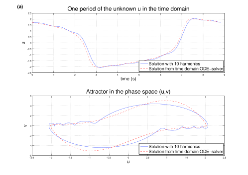
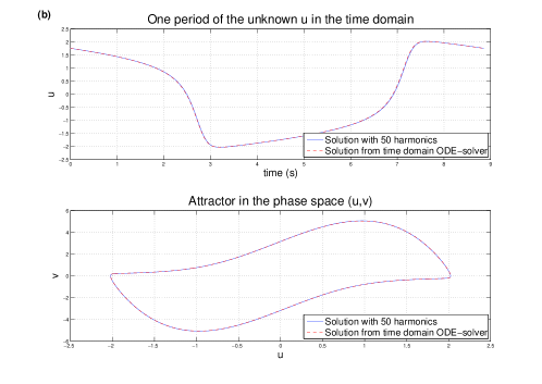
Figure 1: The Van der Pol oscillator (Eq. (4)): Comparison between the harmonic balance results and those obtained with a time domain simulation. Influence of the number of harmonics $H$ taken into account ((a) H=10, (b) H=50).

Example 1: The Van der Pol oscillator. Numerical results obtained on the Van der Pol oscillator (Eq. (4)) are presented in Fig. 1. Good agreement was obtained with the results of a time domain simulation, performed using Matlab ODE solvers. As expected, the number of harmonics $H$ in the solution sought by the harmonic balance method had to be adapted to span the bandwith of the solution obtained by direct integration. In the case of Fig. 1, $\lambda=3$, which requires having a relatively high $H$ to match the reference solution.

Example 2: The Rössler system. The ability to follow period-doubling bifurcations is illustrated in Fig. 2. Following these bifurcations is more difficult in the case of autonomous systems than in forced systems, since the period of oscillation is also unknown. Moreover, since a $T$-periodic solution is also a $2T$-periodic solution, one cannot expect the value of the period obtained by the harmonic balance process to be doubled when crossing a period-doubling bifurcation. The strategy used here therefore consists in introducing complex subharmonic amplitudes as additional unknowns. To detect $K$ period-doubling bifurcations, the solution is then sought as:

$$Z(t)=Z_{0}+\sum_{k=1}^{H}Z_{c,k}\cos(\frac{k}{2^{K}}\omega t)+\sum_{k=1}^{H}Z_{s,k}\sin(\frac{k}{2^{K}}\omega t)$$ (30)

When the solution belongs to the $T$-periodic solution branch, $\left.Z_{c,k}\right|_{k=1..K-1}=0$ and $\left.Z_{s,k}\right|_{k=1..K-1}=0$. When the solution belongs to the $2T$-periodic solution branch, $\left.Z_{c,k}\right|_{k=1..K-1,k\neq 2^{K-1}}=0$ and $\left.Z_{s,k}\right|_{k=1..K-1,k\neq 2^{K-1}}=0$. One practical consequence in terms of the computational cost is that in order to span the same bandwidth, the number of harmonics has be mulitplied by $2^{K}$. This case is illustrated in Fig. 2 where $H=10$ from the $T$-periodic solution to $H=2^{2}\times 10=40$ after two period-doubling bifurcations.

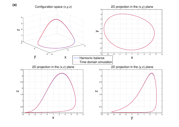
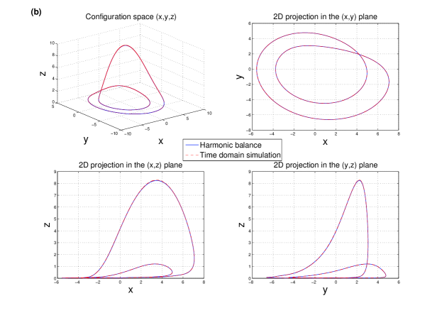
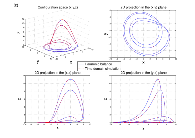
Figure 2: The Rössler system (Eq. (7) with $a=b=0.2$): Comparison between the results obtained using the harmonic balance method and a time domain simulation. These three figures show the ability of the method to follow the sub-harmonic cascade from (a) $\lambda=2.5$ (perdiod $T$), to (b) $\lambda=3.5$ (period $2T$ after a first period-doubling bifurcation) and (c) $\lambda=4$ (period $4T$ after a second period-doubling bifurcation)

Example 3: The clarinet model.

Two typical examples of the bifurcation diagrams obtained with the clarinet model are shown in Fig. 3. These pictures focus on the oscillation threshold in order to show the robustness of the method, even at singular points. As can be seen from both pictures, the radius of convergence of the power series expansion decreases when approaching a bifurcation point (and hence the length of each section of a branch lying between two consecutive points in Fig. 3 decreases). This behaviour is typical of ANM ([33]).

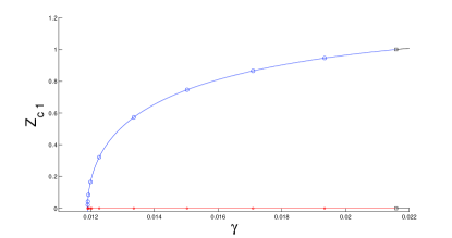
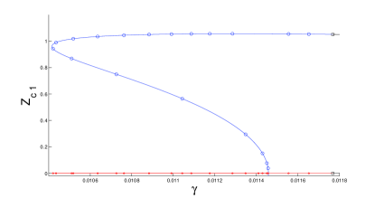
Figure 3: The clarinet model (Eq. (9) with $q_{r}=0.01$, $\omega_{r}=6597$, $H=3$, $N=5$, $c=340$, $\zeta=0.2$, $l_{t}=5.6e-08$, $l_{v}=4e-08$, $C_{pv}=1.4$, $r=0.007$, $w_{1}=2426.5$, $w_{2}=7279.5$, $w_{3}=12132.5$, $w_{4}=16985.4$, $w_{5}=21838.4$, $\alpha_{1}=0.11$, $\alpha_{2}=0.19$, $\alpha_{3}=0.25$, $\alpha_{4}=0.3$, $\alpha_{5}=0.34$): depending on the length of the resonator, the bifurcation will be either a direct Hopf bifurcation (left picture, $L=0.22$) or an inverse Hopf bifurcation (right picture, $L=0.2$).

Example 4: The forced Duffing oscillator

Figure 4 shows the frequency-amplitude diagram of the response obtained with the method presented here. A classical bent resonance curve can be observed, as well as some additional peaks corresponding to superharmonic resonances. Note that only the individual amplitude $A_{i}=\sqrt{(u_{c\;i}^{2}+u_{s\;i}^{2})}$ of the odd harmonics have been plotted, since the even harmonics ($A_{0}$, $A_{2}$, $A_{4}$, $\dots$) are zero. The computation of this branch of periodic orbits required 25 steps of MAN-continuation when 5 harmonics were included, and 35 steps when 9 harmonics were included. The curves obtained for harmonics 1 and 3 were slightly hanged when shifting from $H=5$ to $H=9$ harmonics in Eq. (11). The curve obtained for $A_{5}$ is more affected, which confirms the logical result that more than 5 harmonics have to be used to obtain an accurate result with harmonic $5$. We also checked that the curve obtained for $A_{5}$ was only very slightly modified when shifting from $H=9$ to $H=11$ harmonics in Eq. (11).

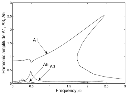
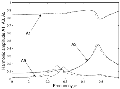
Figure 4: Duffing oscillator, Eq. (24) with $\mu=0.1$ and $f=1.25$ as in ([19]). The figure shows the amplitude of the harmonics 1, 3 and 5 versus the frequency forcing $\omega$. Solid line : results when 5 harmonics are included (H=5 in Eq. (11)). Dash line : results when 9 harmonics are included. The figure on the right is a zoom of the region $\omega<0.6$.

5 Discussion and Conclusion

The key idea in this study is the quadratic recast. It is worth pointing out that the present method contains two quadratic recasts. The first one, which occurs in the time domain, transforms the original system (1) into (3), and is presented in section 2.2. The second one transforms the algebraic system (13) obtained with the HBM, into the final system (17) which is solved by the ANM. The operators in (13) and (17) are linked by (16) and (18). This point accounts for many of the characteristics of the method presented here:

• The whole procedure takes place in the frequency domain using an analytical expression for the system to be solved (as with the classical harmonic balance) and allows to use an arbitrarily high number of harmonics (as with the AFT procedures).

• In the ANM continuation, no iterative process are used to solve the algebraic system, and hence no problems of convergence arise. The computational cost is almost predictible and fairly rather low. On the contrary, convergence of the iterative process can be difficult with AFT procedures ([39, sect. 4.6, p117]).

• There is no need for FFT/IFFT procedures, which increases the computational load in the case of AFT approaches.

• No temporal discretization has to be performed (since the whole procedure is in the frequency domain), and there is therefore no need to cope with aliasing.

• There is no need to use numerical schemes to compute derivatives. Since the problem is a quadratic one , the Jacobian is calculated analytically and this can be done very easily. This is a considerable advantage of the approach presented here. Indeed, as stated by [39, p17], usually "analytical calculation of the Jacobian involves considerable calculation and transformation" but on the other hand, when considering numerical calculation of the Jacobian, "for very nonlinear circuits, the error introduced in the Jacobian estimation results in inaccurate updates of the unknowns and a large number of iterations and possibly no convergence".

As stated in [12], to apply HB, "it is always necessary to write specific computation programs for different nonlinear models". Here, on the contrary, the procedure is simple and rather general because of the natural splitting between the automated part, which is independent of the problem (i.e. the transformation from operators $c,l,q$ to operators ${\bf L}0,{\bf L},{\bf Q}$ and the ensuing solving using the ANM), and the part which depends on the particular problem to be solved (the writing of operators $c,l,q$) which is let to the users. From the point of view of the users, this means that the work required is relatively easy and the software is simple to use. In addition, very few parameters have to be defined by the users: the number of harmonics in the solution and parameter $\epsilon_{r}$ in Eq. (20), which controls the accury of the ANM computation.

In this paper, we have presented only small-sized systems for the sake of simplicity. The method can be obviously extended in principle to large systems of equations although this may require some additional technical work, and introduce limitations due to the lack of computer ressources. In [36], the method has been applied to compute the forced responses of geometrically nonlinear elastic structures discretized using the finite element method. It is well known that with problems of this kind, the equations of motion are second order differential equations in terms of the displacement nodal variables $u$, and that they show a polynomial cubic nonlinarity. Choosing the nodal velocity $v$ and the second Piola-Kirchhoff $S$ (at the Gauss point) as auxiliary variables, the system of equations can easily be written in the form of a first order system with quadratic polynomial non linearities.When a cosine forcing term is applied, they read (in the discrete form)

$$\begin{array}[]{lll}\dot{u}&=&v\\ \mathbf{M}\dot{v}&=&-\int_{V}(B_{L}+B_{NL}(u))^{t}Sdv+\mathbf{F}cos(\lambda t)\\ S&=&D(B_{L}+\frac{1}{2}B_{NL}(u))u\end{array}$$ (31)

where $\mathbf{M}$ is the mass matrix, $D$ is the Hooke operator and $B_{L}$ and $B_{NL}$ are the linear and nonlinear strain-displacement operators [37]. In this form, the governing equations consist in a group of first order differential equations (velocity definition, equation of motion) and a group of algebraic equations (constitutive law at the Gauss point of the finite elements). Both groups are quadratic in $u$ and $S$. The algebra given in annex 1 has been directely introduced into a home-made FEM code, at the element level.

To conclude, it is proposed to discuss the limitations of this method and suggest some possible lines of future research. First of all, it is worth noting that when the original system is not directly in the same quadratic form as Eq. (3), introducting auxiliary variables, as done in this paper, examples may lead to additional (possibly non-physical) solutions. For example, in the case of the clarinet model (example 3), a variable $v=\sqrt{\gamma-p}$ is introduced, and then further defined by the quadratic equation $v^{2}=\gamma-p$. This definition corresponds to $v=\pm\sqrt{\gamma-p}$. In practical terms, this means that the user has to check that the branch of solution computed corresponds to a positive $v$.

The main limitation of the method presented is that the original systems cannot all be put into the quadratic form Eq. (3). For this reason, problems where one or several relations are given in the frequency domain (typically, when some variables are linked through an impedance) cannot be treated. Similar difficulties arise when the original system contains functions (trigonometric functions, exponential functions, non-integer powers function, etc) that are applied to the unknowns. The classical pendulum model $\ddot{\theta}+\sin(\theta)=0$ is a good example of systems of this kind. In these cases, we can generally introduce new variables and new differential equations, so that the functions are generated by the system itself. In the case of pendulum model, $v=\dot{\theta}$ and the two new variables $s(t)=\sin(\theta(t))$ and $c(t)=\cos(\theta(t))$ are introduced. Taking the derivative with respect to time for the last two equations, we obtain

$$\begin{array}[]{lll}\dot{\theta}&=&v\\ \dot{v}&=&-s\\ \dot{s}&=&cv\\ \dot{c}&=&-sv\end{array}$$ (32)

This quadratic system corresponds to the pendulum model, provided the following two initial conditions are added

$$\begin{array}[]{lll}s(0)&=&\sin(\theta(0))\\ c(0)&=&\cos(\theta(0))\end{array}$$ (33)

The application of the HBM to Eq. (32) will now be quite straighforward, but, because of Eq. (33), the final algebraic system will not be quadratic. In these cases, the application of the ANM continuation is still feasible but this requires more elaborate algebra for computating the power series, as explained in ([38, 32]). The efficiency of the present method on the pendulum model will be tested in a near future. Another interesting idea would be to test whether this method can be used to solve regularized non-smooth dynamic problems, and for instance, the case of vibrating systems with contact conditions and friction laws.

Appendix A Appendix

Here, we give the expression for the operators $M$, $C$, $L$ and $Q$ in Eq. (13) in terms of $m$, $c$, $l$, $q$ and $H$. We recall that Eq. (13) is obtained by substituting Eq. (11) into Eq. (3) and by collecting the terms with the same harmonic index (cosines and sines). The inputs of $M$, $L$ and $Q$ are the vector $U$, which contains the Fourier coefficients of $Z(t)$

$$U=[Z_{0}^{t},Z_{c,1}^{t},Z_{s,1}^{t},Z_{c,2}^{t},Z_{s,2}^{t},\dots,Z_{c,H}^{t},Z_{s,H}^{t}]^{t}$$ (34)

A.1 Constant term

The constant vector $c$ is associated with the harmonic zero. The operator $C$ is simply

$$C=[c^{t},0^{t},0^{t},\dots]^{t}$$ (35)

A.2 Linear term

For the linear operator $l$, we have

$$\begin{array}[]{ll}l(Z(t))&=l(Z_{0}+\sum_{k=1}^{H}Z_{c,k}\cos(k\omega t)+Z_{s,k}\sin(k\omega t))\\ &=l(Z_{0})+l(Z_{c,1})\cos(\omega t)+l(Z_{s,1})\sin(\omega t)+l(Z_{c,2})\cos(2\omega t)+\dots\end{array}$$ (36)

The operator $L$ is

$$\small L(U)=[l(Z_{0})^{t},l(Z_{c,1})^{t},l(Z_{s,1})^{t},l(Z_{c,2})^{t},l(Z_{s,2})^{t},\dots,l(Z_{c,H})^{t},l(Z_{s,H})^{t}]^{t}$$ (37)

For the linear operator $m$, we have

$$\begin{array}[]{lll}m(\dot{Z}(t))&=&m(\sum_{k=1}^{H}Z_{s,k}k\omega\cos(k\omega t)-Z_{c,k}k\omega\sin(k\omega t))\\ &=&0+m(Z_{s,1})\omega\cos(\omega t)-m(Z_{c,1})\omega\sin(\omega t)\\ &&+2m(Z_{s,2})\omega\cos(2\omega t)+\dots\end{array}$$ (38)

The operator $M$ is

$$\begin{array}[]{lll}M(U)&=&[0^{t},m(Z_{s,1})^{t},-m(Z_{c,1})^{t},2m(Z_{s,2})^{t},-2m(Z_{c,2})^{t},\dots\\ &&\dots,Hm(Z_{s,H})^{t},-Hm(Z_{c,H})^{t}]^{t}\end{array}$$ (39)

A.3 Quadratic term

With the notation $Z^{(0)}=Z_{0}$ and $Z^{(i)}=Z_{c,i}\cos(\omega t)+Z_{s,i}\sin(\omega t)$, the decomposition of $Z(t)$ is conveniently rewritten as

$$Z(t)=\sum_{i=0}^{H}Z^{(i)}$$ (40)

For the operator $q$, we have

$$\begin{array}[]{ll}q(X(t),Y(t))&=\sum_{i=0}^{H}\sum_{j=0}^{H}q(X^{(i)},Y^{(j)})\\ &=q(X^{(0)},Y^{(0)})+\sum_{i=1}^{H}q(X^{(i)},Y^{(0)})\\ &+\sum_{j=1}^{H}q(X^{(0)},Y^{(j)})+\sum_{i=1}^{H}\sum_{j=1}^{H}q(X^{(i)},Y^{(j)})\\ \end{array}$$ (41)

When $i\geq 1$ and $j\geq 1$, $q(X^{(i)},Y^{(j)})$ give harmonics $i+j$ and $i-j$ as follows:

$$\begin{array}[]{ll}q(X^{(i)},Y^{(j)})&=\frac{1}{2}\{q(X_{c,i},Y_{c,j})-q(X_{s,i},Y_{s,j})\}\cos((i+j)\omega t)\\ &+\frac{1}{2}\{q(X_{c,i},Y_{s,j})+q(X_{s,i},Y_{c,j})\}\sin((i+j)\omega t)\\ &+\frac{1}{2}\{q(X_{c,i},Y_{c,j})+q(X_{s,i},Y_{s,j})\}\cos((i-j)\omega t)\\ &+\frac{1}{2}\{q(X_{s,i},Y_{c,j})-q(X_{c,i},Y_{s,j})\}\sin((i-j)\omega t)\end{array}$$ (42)

By grouping the terms with the same harmonics index, and canceling any harmonics higher than index $H$, we have

$$q(X(t),Y(t))=q_{0}+\sum_{k=1}^{H}q_{c,k}\cos(k\omega t)+q_{s,k}\sin(k\omega t)\\$$ (43)

with

$$q_{0}=q(X_{0},Y_{0})+\sum_{j=1}^{H}\frac{1}{2}\{q(X_{c,j},Y_{c,j})+q(X_{s,j},Y_{s,j})\}$$ (44)

and when $i\geq 1$

$$\begin{array}[]{ll}q_{c,i}&=\{q(X_{c,i},Y_{0})+q(X_{0},Y_{c,i})\}+\sum_{j=1}^{i-1}\frac{1}{2}\{q(X_{c,j},Y_{c,i-j})-q(X_{s,j},Y_{s,i-j})\}\\ +&\displaystyle\sum_{j=i+1}^{H}\frac{1}{2}\{q(X_{c,j},Y_{c,j-i})+q(X_{s,j},Y_{s,j-i})\}+\frac{1}{2}\{q(X_{c,j-i},Y_{c,j})+q(X_{s,j-i},Y_{s,j})\}\\ \end{array}$$ (45)

$$\begin{array}[]{ll}q_{s,i}&=\{q(X_{s,i},Y_{0})+q(X_{0},Y_{s,i})\}+\sum_{j=1}^{i-1}\frac{1}{2}\{q(X_{c,j},Y_{s,i-j})+q(X_{s,j},Y_{c,i-j})\}\\ +&\displaystyle\sum_{j=i+1}^{H}\frac{1}{2}\{-q(X_{c,j},Y_{s,j-i})+q(X_{s,j},Y_{c,j-i})\}+\frac{1}{2}\{q(X_{c,j-i},Y_{s,j})-q(X_{s,j-i},Y_{c,j})\}\\ \end{array}$$ (46)

References

- [1] A. H. Nayfeh and D.T. Mook, Nonlinear oscillations, Wiley series in nonlinear science, 1979.
- [2] W. Szemplinska-stupnicka, The behaviour of nonlinear vibrating systems -Vol I- fondamental concepts and methods : application to single-degree-of-freedom systems, Kluwer academic publishers, 1990.
- [3] R. Seydel, From equilibrium to Chaos, Practical bifurcation and stability analysis, Interdisciplinary Applied Mathematics (Vol 5) Springer Verlag, 1994.
- [4] A. H. Nayfeh and B. Balachandran, Applied Nonlinear Dynamics: Analytical Computational and Experimental Methods, Wiley series in nonlinear science, 1995.
- [5] E. Doedel and H.B. Keller and J.P. Kernevez, Numerical Analysis and Control of Bifurcation Problems (I) Bifurcation in Finite Dimensions, International Journal of Bifurcation and Chaos 1(1991) 439-528.
-
[6]
http://manlab.lma.cnrs-mrs.fr/(last successfully accessed, 17th dec. 2008). - [7] E.J. Doedel, Lecture notes on numerical analysis of nonlinear equations, in: B. Krauskopf, H.M. Osinga and J. Galan-Vioque (Eds.), Numerical Continuation methods for dynamical systems, Springer Verlag, 2007, pp.1-49.
- [8] Krylov and Bogoliubov, Introduction to Nonlinear Mechanics, Princeton University Press, New Jersey, 1947, English translation of Russian edition from 1936.
- [9] M. Urabe, Galerkin’s procedure for nonlinear periodic systems, Arch. for Rational Mechanics and Analysis 20(1965) 120-152.
- [10] A. Stokes, On the approximation of nonlinear oscillations, Journal of differential equations 12(1972) 535-558.
- [11] M. S. Nakhla and J. Vlach, A piecewise harmonic balance technique for determination of periodic response of nonlinear systems, IEEE Trans. Circuit Theory 23(1976) 85-91.
- [12] Z.K. Peng, Z.Q. Lang, S.A. Billings, G.R. Tomlinson, Comparisons between harmonic balance and nonlinear output frequency response function in nonlinear system analysis, Journal of Sound and Vibration 311(2008) 56-73.
- [13] S.L. Lau , Y.K. Cheung , Amplitude incremental variational principle for nonlinear vibration of elastic systems, ASME Journal of Applied Mechanics 28(1981) 959-964.
- [14] V. P. Iu , Y.K. Cheung , Non linear vibration analysis of multilayer sandwich plates by incremental finite elements, Part I Theoretical development, Engineering Computation 3(1986) 36-42.
- [15] C. Pierre, A. A. Ferri, H. Dowell , Multi-harmonic analysis of dry friction damped systems using an incremantal harmonic balance method, ASME Journal of Applied Mechanics 52(1985) 958-964.
- [16] F.H. Ling, X.X. Wu , Fast Galerkin method and its application to determine periodic solutions of non-linear oscillators, International Journal of Non-linear Mechanics 22(1987) 89-98.
- [17] S. Navicet, C. Pierre, F. Thouverez, L. Jéséquel, A dynamic Lagrangian frequency-time method for the vibrations of dry-friction-damped systems, Journal of Sound and Vibration 265(2003) 201-219.
- [18] S.K. Lay, C.W. Lim, B.S. Wu, C. Wang, Q.C. Zeng, X.F. He, Newton-harmonic balancing approach for accurate solutions to nonlinear cubic and quintic Duffing oscillators, Appl. Math. Modell. (to appear).
- [19] L. Liu, J.P. Thomas, E.H. Dowell, P. Attar, K.C. Hall, A comparison of classical and high dimensional harmonic balance approaches for a Duffing oscillator, Journal of Computational Physics 215(2006) 298-320.
- [20] N. Damil and M. Potier-Ferry, A new method to compute perturbed bifurcation: Application to the buckling of imperfect elastic structures, International Journal of Engineering Sciences 26(1990) 943-957.
- [21] L. Azrar and B. Cochelin and N. Damil and M. Potier-Ferry, An asymptotic-numerical method to compute the post-buckling behaviour of elastic plates and shells, International Journal for Numerical Methods in Engineering 36(1993) 1251-1277.
- [22] B. Cochelin and N. Damil and M. Potier-Ferry, Asymptotic-Numerical Method and Padé approximants for non-linear elastic structures, International Journal for Numerical Methods in Engineering 37(1994) 1187-1213.
- [23] B. Cochelin, A path-following technique via an asymptotic-numerical method, Computers and Structures 53(1994) 1181-1192.
- [24] B. Cochelin and N. Damil and M. Potier-Ferry, The asymptotic-numerical method : an efficient perturbation technique for nonlinear structural mechanics, Revue Européenne des Eléments Finis 3(1994) 281-297.
- [25] H. Zahrouni and B. Cochelin and M. Potier-Ferry, Computing finite rotation of shells by an asymptotic-numerical method, Computer Methods in Applied Mechanics and Engineering 175(1999) 71-85.
- [26] L. Azrar and R. Benamar M. Potier-Ferry, An asymptotic-numerical method for large amplitude free vibrations of thin elastic plates, Journal of sound and vibration 220(1999) 625-727.
- [27] J.M. Cadou and B. Cochelin and N. Damil and M. Potier-Ferry, ANM for stationary Navier-Stokes equations with Petrov-Galerkin formulation, International Journal for Numerical Methods in Engineering 50(2001) 825-845.
- [28] F. Silva, V. Debut, J. Kergomard, C. Vergez, A. Deblevid, P. Guillemain, Simulation of single reed instruments oscillations based on modal decomposition of bore and reed dynamics, Proceedings of the International Congress of Acoustics, Madrid, Spain.
- [29] E.L. Allgower, K.G. Georg, Numerical continuation methods, an introduction, Springer series in Computational Mathematics (Vol 13), Springer-Verlag, 1990.
- [30] B. Krauskopf H.M. Osinga J. Galan-Vioque Eds, Numerical Continuation methods for dynamical systems, Path following and boundary value problems, Springer Verlag, 2007.
- [31] W. Govaerts and Y. Kuznetsov, Interactive continuation tools, in: B. Krauskopf, H.M. Osinga and J. Galan-Vioque (Eds), In Numerical Continuation methods for dynamical systems, Springer Verlag, 2007, pp.51-75.
- [32] B. Cochelin , N. Damil , M. Potier-Ferry., Méthode Asymptotique Numérique, Collection méthodes numériques, Hermes Sciences Lavoisier, 2007, in French.
- [33] S. Baguet and B. Cochelin, On the behaviour of the ANM continuation in the presence of bifurcation, Communication in Numerical Methods in Engineering 19(2003) 459-471.
- [34] R. Arquier, Une méthode de calcul des modes de vibrations nonlinéaires de structures, PhD Thesis, Université de la méditerranée, Marseille, 2007.
- [35] M.S. Plesset, The dynamics of cavitation bubbles, Journal of Applied Mechanics 16(1949) 277-282.
- [36] F. Pérignon and S. Bellizzi and B. Cochelin, Numerical and experimental analysis of nonlinear forced vibrations of imperfect plates, Proceedings of the ISMA conference, Louvain, 2002.
- [37] M. Crisfield, Non-linear finite element analysis of solids and structures, John Wiley and Sons, New York, Vol. 1, 1991.
- [38] M.Potier-Ferry and N. Damil and B. Braikat and J. Descamps and J.M. Cadou and H.L. Cao and A.E. Hussein, Traitement des fortes non-linéarités par la méthode asymptotique numérique, Comptes rendus de l’Académie des Sciences, Paris 324(1997) Serie IIb 171-177.
- [39] B. Troyanovsky, Frequency Domain Algorithms for simulating large signal distortion in semiconductor devices, PhD Thesis, Stanford University, 1997.