Accelerometer using atomic waves for space
applications

Abstract

The techniques of laser cooling combined with atom interferometry make possible the realization of very sensitive and accurate inertial sensors like gyroscopes or accelerometers. Besides earth-based developments, the use of these techniques in space should provide extremely high sensitivity for research in fundamental physics, Earth’s observation and exploration of the solar system.

1 Introduction

Inertial sensors are useful devices in both science and industry. Higher precision sensors could find scientific applications in the areas of general relativity [1], geodesy and geology. There are also important applications of such devices in the field of navigation, surveying and analysis of earth structures. Matter-wave interferometry was envisaged for its potential to be an extremely sensitive probe for inertial forces [2]. In 1991, atom interference techniques have been used in proof-of-principle work to measure rotations [3] and accelerations [4]. In the following years, many theoretical and experimental works have been performed to investigate this new kind of inertial sensors [5]. Some of the recent works have shown very promising results leading to a sensitivity comparable to other kinds of sensors, as well as for rotation [6] as for acceleration [7] and possibility of realizing a full inertial base within the same device [8]. The most developed atom-interferometer inertial sensors are today atomic state interferometers [9] which use two-photon velocity selective Raman transitions [10, 11] to manipulate atoms while keeping them in long-lived ground states.

Atom interferometry is nowadays one of the most promising candidates for ultra-precise and ultra-accurate measurement of gravito-inertial forces on ground or for space [12]. From performances on ground, one can expect unprecedented sensitivity in space, leading to many mission proposals since 2000 [13]. This technology is now mature enough that several groups are developing instruments for practical experiments: in the field navigation  [14], or fundamental physics (gradiometer for the measurement of G [15], gravimeter for the watt balance experiment [16], interferometer for the measurement of fine structure constant thanks to $h/m$ [17]). Moreover, the realization of Bose-Einstein condensation (BEC) of a dilute gas of trapped atoms in a single quantum state [18, 19, 20] has produced the matter-wave analog of a laser in optics [21, 22, 23, 24] and open new possibilities. Alike the revolution brought by lasers in optical interferometry [1, 25, 26], it is expected that the use of Bose-Einstein condensed atoms will bring the science of atom optics, and in particular atom interferometry, to an unprecedented level of accuracy [27, 28]. In addition, BEC-based coherent atom interferometry would reach its full potential in space-based applications where micro-gravity will allow the atomic interferometers to reach their best performance. Applications of accelerometer in space concern fundamental physics, like testing the equivalence principle by comparing the free fall of two different atomic species [29], and more generally testing all aspects of gravity as in [30], which aims at testing the laws of gravity at large scale, as well for fundamental physics as for exploration of the solar system.

In the following part, we investigate the sources of noise and systematic effects for such atom interferometers, thanks to the results obtained with the gravimeter under development in our laboratory. This setup is based on same concepts than previous works [7]: atomic source realized with a magneto-optical traps and manipulation of the atomic wavepackets with Raman transitions. In our experiment, we have studied in details the influence of any perturbations on the sensitivity of the sensor. Reducing there impacts on the noise of the instrument, we finally reach an excellent sensitivity of $1.4\times 10^{-8}\,\rm{m.s^{-2}.Hz^{-1/2}}$, despite a rather short interrogation time ($100\;{\rm ms}$ only). We think this experiment is a good benchmarck to oversee the performances of best space accelerometers based on same technologies. Performances in space environment will be derived, taking into account the specifications of the environment and the much longer interrogation time.

2 Experimental setup

The principle of our gravimeter is based on the coherent splitting of matter-waves by the use of two-photon Raman transitions [31]. These transitions couple the two hyperfine levels $F=1$ and $F=2$ of the ${}^{5}S_{1/2}$ ground state of the ⁸⁷Rb atom. An intense beam of slow atoms is first produced by a 2D-MOT. Out of this beam $10^{7}$ atoms are loaded within 50 ms into a 3D-MOT and subsequently cooled in a far detuned (-25 $\Gamma$) optical molasses. The lasers are then switched off adiabatically to release the atoms into free fall at a final temperature of $2.5~{}\mu\textrm{K}$. Both lasers used for cooling and repumping are then detuned from the atomic transitions by about 1 GHz to generate the two off-resonant Raman beams. For this we have developed a compact and agile laser system that allows us to rapidly change the operating frequencies of these lasers, as described in [32]. Before entering the interferometer, atoms are selected in a narrow vertical velocity distribution ($\sigma_{v}\leq v_{r}=5.9$ mm/s) in the $\left|F=1,m_{F}=0\right\rangle$ state, using a combination of microwave and optical Raman pulses.

The interferometer is created by using a sequence of three pulses ($\pi/2-\pi-\pi/2$), which split, redirect and recombine the atomic wave packets. Thanks to the relationship between external and internal state [9], the interferometer phase shift can easily be deduced from a fluorescence measurement of the populations of each of the two states. Indeed, at the output of the interferometer, the transition probability $P$ from one hyperfine state to the other is given by the well-known relation for a two wave interferometer: $P=\frac{1}{2}\left(1+C\cos\Delta\Phi\right)$, where $C$ is the interferometer contrast, and $\Delta\Phi$ the difference of the atomic phases accumulated along the two paths. The difference in the phases accumulated along the two paths depends on the acceleration $\vec{a}$ experienced by the atoms. It can be written as [31] $\Delta\Phi=\phi(0)-2\phi(T)+\phi(2T)=-\vec{k}_{eff}\cdot\vec{a}T^{2}$, where $\phi(0,T,2T)$ is the difference of the phases of the lasers, at the location of the center of the atomic wavepackets, for each of the three pulses [33]. Here $\vec{k}_{eff}=\vec{k}_{1}-\vec{k}_{2}$ is the effective wave vector (with $|\vec{k}_{eff}|=k_{1}+k_{2}$ for counter-propagating beams), and $T$ is the time interval between two consecutive pulses.

The Raman light sources are two extended cavity diode lasers based on the design of [34], which are amplified by two independent tapered amplifiers. Their frequency difference is phase locked onto a low phase noise microwave reference source. The two overlapped beams are injected in a polarization maintaining fiber, and guided towards the vacuum chamber. We obtain counter-propagating beams by placing a mirror and a quarterwave plate at the bottom of the experiment. Four beams are actually sent onto the atoms, out of which only two will drive the counter-propagating Raman transitions, due to conservation of angular momentum and the Doppler shift induced by the free fall of the atoms.

Experimental setups, based on the same principle, can be realized for space experiments. They will benefit from the technical developments realized in the frame of the PHARAO atomic clock [35] for the space ACES project.

3 Sensitivity of the interferometer

3.1 Sensitivity function

The sensitivity function characterizes the influence of fluctuations in the Raman lasers phase difference $\phi$ onto the transition probability [36], and thus on the interferometer phase. This function is defined by :

$$\ g(t)=2\lim_{\delta\phi\rightarrow 0}\frac{\delta P(\delta\phi,t)}{\delta\phi}.\$$ (1)

where $\delta\phi$ is a jump on the Raman phase difference $\phi$, which occurs at time t during the interferometer sequence, and induces a change of $\delta P(\delta\phi,t)$ in the transition probability.

The expression of the sensitivity function can easily be derived when considering that the Raman pulses are infinitesimally short. In that case, the interferometer phase $\Phi$ is given by [4]: $\Phi=\phi_{1}-2\phi_{2}+\phi_{3}$, where $\phi_{1}$,$\phi_{2}$,$\phi_{3}$ are the the Raman laser phase differences at the three laser interactions, taken at the position of the center of the atomic wavepacket [33]. Usually, the interferometer is operated at mid fringe ($\Phi=\pi/2$), in order to maximize the sensitivity to interferometer phase fluctuations. If the phase step $\delta\phi$ occurs for instance between the first and the second pulses, the interferometric phase changes by $\delta\Phi=-\delta\phi$, and the transition probability by $\delta P=-cos(\pi/2+\delta\Phi)/2\sim-\delta\phi/2$ in the limit of an infinitesimal phase step. Thus, in between the first two pulses, the sensitivity function is -1. The same way, one finds for the sensitivity function between the last two pulses : +1.

In the more general case of finite duration Raman laser pulses, the sensitivity function will depend on the time evolution of the atomic state during the pulses. This function is calculated in [37] considering laser waves as plane waves and quantizing atomic motion in the direction parallel to the laser beams, in the case of a constant Rabi frequency (square pulses) and resonance condition fulfilled. We calculated the change in the transition probability for a infinitesimally small phase jump at any time t during the interferometer, and deduce $g(t)$.

The sensitivity function is an odd function, whose expression is given here for $t>0$:

$$g(t)=\left\{\begin{array}[]{ll}\sin(\Omega_{R}t)&0<t<\tau_{R}\\ 1&\tau_{R}<t<T+\tau_{R}\\ -\sin(\Omega_{R}(T-t))&T+\tau_{R}<t<T+2\tau_{R}\\ \end{array}\right.$$ (2)

where we choose the time origin at the middle of the second Raman pulse and where $\Omega_{R}/2\pi$ is the Rabi frequency.

Using this function, we can now evaluate the fluctuations of the interferometric phase $\Phi$ for an arbitrary Raman phase noise $\phi(t)$ on the lasers

$$\delta\Phi=\int_{-\infty}^{+\infty}g(t)d\phi(t)=\int_{-\infty}^{+\infty}g(t)\frac{d\phi(t)}{dt}dt.$$ (3)

3.2 Influence of the phase noise onto the sensitivity of the interferometer

The sensitivity of the interferometer is characterized by the Allan variance of the interferometer phase fluctuations, $\sigma^{2}_{\Phi}(\tau)$, defined as

$$\sigma_{\Phi}^{2}(\tau) = \frac{1}{2}\langle(\bar{\delta\Phi}_{k+1}-\bar{\delta\Phi}_{k})^{2}\rangle$$ (4)

$$= \frac{1}{2}\lim_{n\rightarrow\infty}\left\{\frac{1}{n}\sum_{k=1}^{n}(\bar{\delta\Phi}_{k+1}-\bar{\delta\Phi}_{k})^{2}\right\}.$$ (5)

where $\bar{\delta\Phi}_{k}$ is the average value of $\delta\Phi$ over the interval $[t_{k},t_{k+1}]$ of duration $\tau$. The Allan variance is equal, within a factor of two, to the variance of the differences in the successive average values $\bar{\delta\Phi}_{k}$ of the interferometric phase. As the interferometer is operated sequentially at a rate $f_{c}=1/T_{\rm{c}}$, $\tau$ is a multiple of $T_{c}$ : $\tau=mT_{c}$.

In order to evaluate correctly the stability of the interferometer phase $\Phi$, it is necessary to take into account that the measurement is pulsed. The sensitivity of the interferometer is limited by an aliasing phenomenon, similar to the Dick effect for atomic clocks [36]: only the phase noise at multiples of the cycling frequency contribute to the Allan variance, weighted by the Fourier components of the transfer function. For large averaging times $\tau$, the Allan variance of the interferometric phase is given by

$$\sigma^{2}_{\Phi}(\tau)={1\over\tau}\sum_{n=1}^{\infty}|H(2\pi nf_{\rm{c}})|^{2}S_{\phi}({2\pi nf_{\rm{c}}})$$ (6)

where $S_{\phi}(\omega)$ is the power spectral density of the Raman phase, and $H(\omega)$ is the transfer function, given by $H(\omega)=\omega G(\omega)$, where $G$ is the Fourier transform of the sensitivity function.

$$G(\omega)=\int_{-\infty}^{+\infty}e^{-i\omega t}g(t)dt$$ (7)

At low frequency ($\omega<<\Omega_{R}$), $G$ can be approximated by

$$G(\omega)=-\frac{4i}{\omega}\sin^{2}[\omega(T+2\tau_{R})/2]$$ (8)

The transfer function $|H^{2}|$ has two important features. First, it presents oscillations at a frequency given by $1/(T+2\tau_{R})$, leading to zeros at frequencies given by $f_{k}=\frac{k}{T+2\tau_{R}}$. The second is a low pass first order filtering due to the finite duration of the Raman pulses.

For white phase noise $S_{\phi}^{0}$, and to first order in $\tau_{R}/T$, the phase stability is given by:

$$\sigma^{2}_{\Phi}(\tau)=\frac{\pi\Omega}{2}S_{\phi}^{0}\frac{T_{c}}{\tau}$$ (9)

where $\Omega$ is the Rabi frequency.

This illustrates the filtering of the transfer function: the shorter the pulse duration $\tau_{R}$, the greater the interferometer noise.

3.3 The 100 MHz source oscillator

To reduce the noise of the interferometer, the frequency difference between the Raman beams needs to be locked to a very stable microwave oscillator, whose frequency is close to the hyperfine transition frequency ($\nu_{mw}=6.834$ GHz for ⁸⁷Rb). The reference frequency will be delivered by a frequency chain, which transposes in the microwave domain the low phase noise of an RF oscillator, typically a quartz oscillator. When this transposition is performed without degradation, the phase noise power spectral density of the RF oscillator, of frequency $\nu_{rf}$, is multiplied by $(\nu_{mw}/\nu_{rf})^{2}$.

No single quartz oscillator fulfills the requirements of ultra low phase noise over a sufficiently large frequency range. We present in figure 1 the specifications for different high stability quartz : a Premium 10 MHz-SC from Wenzel, a BVA OCXO 8607-L from Oscilloquartz, and a Premium 100 MHz-SC quartz from Wenzel. The phase noise spectral density is displayed at the frequency of 100 MHz, so that one can compare the different quartz oscillators.

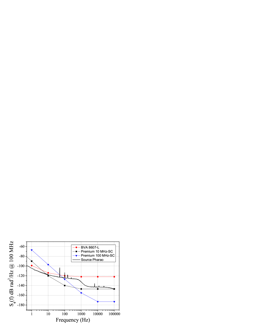
Figure 1: Specifications for the phase noise spectral density of different quartz oscillators, transposed at 100 MHz. The phase noise of the source developed for the Pharao project is also displayed as a solid black line.

A 100 MHz source for a space interferometer could be realized by combining two quartz oscillators. A 100 MHz quartz would be locked onto one of the above mentioned high stability 10 MHz reference oscillators. The bandwidth of this lock will correspond to the frequency below which the phase noise of the reference quartz is lower than the noise of the 100 MHz quartz.

The phase noise properties of such a combined source can be seen in figure 1, where we display as a solid line the phase noise spectral density of the 100 MHz source developed by THALES for the PHARAO space clock project. This combined source has been optimized for mimimal phase noise at low frequency, where it reaches a level of noise lower than any commercially available quartz. An atomic clock is indeed mostly limited by the lower frequency part of the frequency spectrum, so the requirements on the level of phase noise at higher frequency ($f>1$kHz) is less stringent than for an atom interferometer. A medium performance 100 MHz oscillator is thus sufficient.

Using a simple model for the phase lock loop, we calculated the phase noise spectral density of the different combined sources we can realize by locking the Premium 100 MHz-SC either on the Premium 10 MHz-SC (Source 1), or on the BVA (source 2), or even on the Pharao source (source 3). We then estimated the impact on the interferometer of the phase noise of the 100 MHz source, assuming we are able to transpose the performance of the source at 6.8 GHz without degradation. We calculated using 6 the Allan standard deviation of the interferometric phase fluctuations for the different configurations and for various interferometer parameters. The results are presented in table 1.

			Source 1	Source 2	Source 3
$T_{c}$	$2T$	$\tau_{R}$	$\sigma_{\Phi}$($T_{c}$)	$\sigma_{\Phi}$($T_{c}$)	$\sigma_{\Phi}$($T_{c}$)
(s)	(s)	($\mu$s)	(mrad)	(mrad)	(mrad)
0.25	0.1	10	1.2	3.5	2.2
3	2	10	21	6.5	4.4
15	10	10	110	37	19

Table 1: Contribution of the 100 MHz source phase noise to the interferometrer phase fluctuations. The calculation has been performed for a Rb interferometer, for each of the three different sources and for various parameters of the interferometer. First case corresponds to the usual parameters of our gravimeter, and second (resp. third) case corresponds to typical values for space experiments with a MOT atomic source (resp. ultra-cold source).

For short interrogation times (such as $2T=100$ ms, which is the maximum interrogation time of our cold gravimeter), Source 1 behaves better, whereas for large interrogation times, where the dominant contribution to the noise comes from the lower decades (0.1-10 Hz), Source 2 and 3 are better. We assumed here that for any of these sources, the phase noise below 1 Hz is well described as flicker noise, for which the spectral density scales as $S_{\phi}(f)=S_{\phi}(1\rm{Hz})/f^{3}$. If the phase noise would behave as pure flicker noise over the whole frequency spectrum, the Allan standard deviation of the interferometer phase would scale as $T$. This is roughly the behavior we notice in the table for long interrogation times.

The sensitivity of the interferometer for acceleration scales as $T^{2}$, so that the sensitivity to acceleration gets better when the interrogation time gets larger. For example, for $2T=10$s and $T_{c}=15$ s (resp. $2T=2$ s and $T_{c}=3$ s), the phase noise of source 3 would limit the sensitivity to acceleration of the interferometer to $1.8\times 10^{-10}\rm{m.s}^{-2}$ (resp. $4.7\times 10^{-10}\rm{m.s}^{-2}$) at 1 s for ${}^{87}Rb$.

3.4 The frequency chain

The microwave signal is generated by multiplication of the 100 MHz source. An example of the generation of the microwave reference can be found in [38]. The contribution to the interferometer noise of this system was found to be 0.6 mrad per shot for $\tau_{R}=10\mu$ s, $2T=10$ s and $T_{c}=15$ s, which is negligible with respect to the contribution from the 100 MHz source.

3.5 Propagation in the fiber

In most of the experiment, the Raman lasers are generated by two independent laser sources. The two beams are mixed using a polarizing beam splitter cube, so that they have orthogonal polarizations. A small fraction of the total power can be sent to one of the two exit ports of the cube, where a fast photodetector detects the beat frequency, in order to phase lock the lasers. Both beams are finally guided towards the atoms with a polarization maintaining fiber. Since the Raman beams have orthogonal polarization, fiber length fluctuations induce phase fluctuations, due to the birefringence of the medium. The phase noise induced by the propagation in the fiber can be measured by comparing the beat signal measured after the fiber with the one we use for the phase lock.

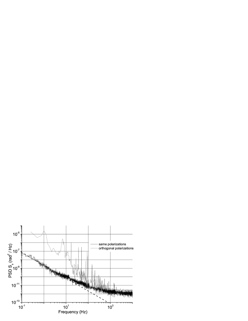
Figure 2: Contribution of the propagation in the optical fiber to the Raman phase noise. Grey curve displays the noise in the case of a polarization maintaining fiber and two orthogonal polarizations for the two Raman lasers. Black curve displays the noise in the case of a polarizing fiber and two parallel polarizations for the two Raman lasers.

Figure 2 displays the power spectral density of the phase noise induced by the propagation, which is dominated by low frequency noise due to acoustic noise and thermal fluctuations. This source of noise can be reduced by shielding the fiber from the air flow of the air conditioning, surrounding it with some packaging foam. An alternative technique consists in using identical linear polarizations for the Raman beams. This can be achieved using a polarizer after the mixing, by generating the Raman lasers by phase modulatuion of a single laser, or by injecting with two independent lasers a power amplifier. In this case, the noise is efficiently suppressed, as shown in figure 2, down to a level where it is negligible.

3.6 Detection noise

Quantum projection noise limit constitutes the intrinsic limit of sensitivity and scales as $1/\surd{N}$, where N is the number of detected atoms per shot. Typical values are below 1 mrad for MOT sources and 3 mrad for ultra cold atomic sources. Thus for long interrogation times, as for space applications, the dominant source of phase noise is expected to be due to the stability of the 100 MHz source.

4 The case of parasitic vibrations

The same formalism can be used to evaluate the degradation of the sensitivity to inertial forces caused by vibrations of the retroreflecting mirror.

The sensitivity of the interferometer is then given by

$$\sigma^{2}_{\Phi}(\tau)={k_{eff}^{2}\over\tau}\sum_{n=1}^{\infty}|H(2\pi nf_{\rm{c}})|^{2}S_{z}(2\pi nf_{\rm{c}})$$ (10)

where $S_{z}(\omega)$ is the power spectral density of position noise. Introducing the power spectral density of acceleration noise $S_{a}(\omega)$, the previous equation can be written

$$\sigma^{2}_{\Phi}(\tau)={k_{eff}^{2}\over\tau}\sum_{n=1}^{\infty}\frac{|H(2\pi nf_{\rm{c}})|^{2}}{(2\pi nf_{\rm{c}})^{4}}S_{a}(2\pi nf_{\rm{c}})$$ (11)

It is important to note here that the acceleration noise is efficiently filtered by the transfer function for acceleration, which decreases as $1/f^{4}$.

In the case of white acceleration noise $S_{a}$, and to first order in $\tau_{R}/T$, the limit on the sensitivity of the interferometer is given by :

$$\sigma^{2}_{\Phi}(\tau)=\frac{k_{eff}^{2}T^{4}}{2}\left(\frac{2T_{\rm{c}}}{3T}-1\right)\frac{S_{a}}{\tau}\$$ (12)

To put this into numbers, we now calculate the requirements on the acceleration noise of the retroreflecting mirror in order to reach a sensitivity of $\times 10^{-10}\,\rm{m.s^{-2}}$ at 1 s. For negligible dead time ($Tc\simeq 2T)$, the amplitude noise should lie below $2.5\times 10^{-10}\,\rm{m.s^{-2}.Hz^{-1/2}}$.

5 Systematic effects

Regarding the targeted ultra-high accuracies for atom inertial sensors, many environmental parameters have to be controlled with great precision. An important tool, that allows us to suppress many of the remaining systematic phase shifts, relies on the fact that we can distinguish two classes of systematic effects.

Phase shifts that are independent of the direction of $\overrightarrow{k_{eff}}$ and others that change sign when reversing $\overrightarrow{k_{eff}}$. This allows us to separate and distinguish their influence on the atomic signal in constantly repeated $k_{\uparrow}-k_{\downarrow}$ measurements. Assuming that the trajectories of the atoms remain constant, the half difference $\frac{1}{2}\triangle_{\uparrow\downarrow}$ of the measured interferometer phase $\Delta\Phi_{int}$ of a consecutive $k_{\uparrow}-k_{\downarrow}$ measurement will contain only phase terms depending on $\overrightarrow{k_{eff}}$. Whereas $\overrightarrow{k_{eff}}$ independent phase terms are contained in the half sum $\frac{1}{2}{\sum}_{\uparrow\downarrow}$:

$$\frac{1}{2}\triangle_{\uparrow\downarrow}=-\cos\theta|\overrightarrow{k}_{eff}|\cdot|\overrightarrow{g}|\cdot T^{2}+\Delta\Phi_{LS2}+\Delta\Phi_{Coriolis}+\Delta\Phi_{Aberr}+...$$ (13)

$$\frac{1}{2}{\sum}_{\uparrow\downarrow}=\Delta\Phi_{RF}+\Delta\Phi_{LS1}+\Delta\Phi_{gradB}+...$$ (14)

5.1 k-independent Phase Shifts

Three major contributions to large phase shifts in the interferometer, that can be rejected from the $k$-dependent acceleration signal, $-\overrightarrow{k_{eff}}\cdot\overrightarrow{g}\,{T}^{2}$, arise from the presence of magnetic field gradients, 1-photon light shifts [39] and RF-phase shifts (see equ. (14)).

We have experimentally demonstrated this rejection on our cold atom gravimeter. To test the rejection of k-independent phase shifts from the actual atomic signal, we have performed differential measurements with 4 configurations (two sets of parameters and $k_{\uparrow}-k_{\downarrow}$ each). The difference in their half-sums $\Delta(\frac{1}{2}\sum)$ gives us the additionally introduced phase shift. The difference in their half-differences $\Delta(\frac{1}{2}\triangle)$ shows the remaining phase error, that is not rejected by the $k_{\uparrow}-k_{\downarrow}$ measurement.

With this method, we demonstrated rejection efficiencies typically better than 99%, limited by the resolution of the measurement (in the case of the RF and 1-photon light shift), and by the imperfect overlap between the atomic trajectories for the $k_{\uparrow}-k_{\downarrow}$ interferometers (in the case of the magnetic field gradient). For a space interferometer, the influence of the magnetic field gradients are expected to be reduced with respect to the case of ground experiment, as i) atoms travel along shorter distances, and ii) the two separated wave-packets experience the same phase shifts, as they alternately travel along identical trajectories.

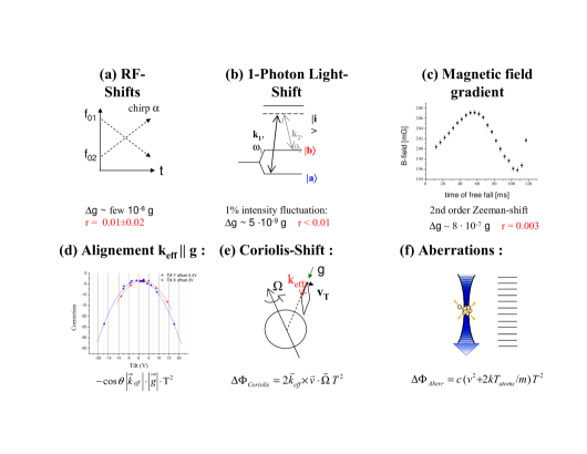
Figure 3: Some major contributions to systematic phase shifts in our cold atom gravimeter. (a)-(c) depend on the direction of $k_{eff}$ and can be rejected to a residual $r$, (d)-(e) are indistinguishable from the acceleration signal and need to be controlled within a high precision.

5.2 k-dependent Phase Shifts

As shown above, large systematic error contributions can be removed from the atomic signal by systematic $k_{\uparrow}$-$k_{\downarrow}$ measurements. The remaining phase shifts in equation (13) are due to effects that are inherently sensitive to the direction of $k$.

The first term in equ. (13) represents the actual atomic signal due to the acceleration of the atoms. The atomic transition wavelength, which is determining $k_{eff}$, is known to better than 1 kHz [40].

Three major sources of phase errors add onto this acceleration induced phase shift. Similar to the 1-photon light shift, the Eigen-energies of the atomic states are modified in higher order terms by 2-photon transitions of the Raman beams themselves (LS2). This 2-photon light shift introduces a phase shift similar to this of the usual 1-photon light shift, but where the shift of the resonance transition is ${\delta\nu_{AC}}^{(LS2)}={\Omega_{eff}}^{2}/\delta_{Doppler}$, and $\delta_{Doppler}=k_{eff}\cdot v$ is the Doppler-detuning of the stimulated Raman transition from resonance.

Term 3 and 4 in equ.(13) are phase terms that both depend on the transverse velocities of the atoms and are difficult to clearly distinguish. Any residual offset velocity $v_{T}$ perpendicular to $\overrightarrow{k_{eff}}$ will lead to phase errors due to Coriolis forces and imperfect plane wave fronts of the Raman beams (aberrations) [41]. As indicated in figure 3(e), a finite $v_{T}$ will lead to a finite area spanned by the interferometer and thus will make it sensitive to rotations.

Contrary to that, phase shifts due to aberrations in the phase fronts of the Raman beams scale with the temperature $T_{atoms}$ of the atomic ensemble, depending on the shape of distortion in the wave fronts. For a in first order parabolic curvature of the wave front $\Delta\Phi=c\cdot r^{2}$, we obtain $\Delta\Phi_{Aberr}=c\,(v_{T}^{2}+2\,k_{B}\,T_{atoms}/m)T^{2}$. Here, the interferometer is only sensitive to perturbations introduced in the retro-reflected beam path, which is non-common to both Raman laser beams. In case of a pure curvature of the retro-reflected phase fronts, $\Delta a=10^{-10}$ m/s² would require $c=17$ rad/m², which corresponds to a phase front radius of $R=240$ km, or a flatness of $\approx\lambda/1500$ over a beam diameter of 10 mm. This flatness is difficult to reach, especially with retardation plates.

Irregularly shaped phase distortions, as introduced by mirror and $\lambda/4$ plate, can average out and the requirement for the surface flatness is less stringent. To deduce the effect on the atomic signal, the wave front distortion introduced by the individual optical elements have to be measured with a Shack-Hartmann sensor or ZYGO interferometer, at the level of $\approx\lambda/1000$ or better. The collected phase shifts along the classical trajectories of the atoms can then be calculated. Measurements of the phase shift of the interferometer versus initial position and velocity, and versus temperatures can be useful to study this systematic effect, and correct for it.

In space, Coriolis acceleration could also be an issue, depending on the details of the mission. One should though keep in mind that this bias is not intrinsic to the device, but is a part of the signal and is related to the actual trajectory of the satellite. Wavefront aberrations appear as a very important systematic effect, which depends on a non trivial way with the experimental parameters (size and temperature of the atomic cloud and interaction time). To overcome this problem, extremely high flatness optics are required.

6 Conclusion

Thanks to a careful study and optimization of all sources of noise and systematics on our gravimeter, we can evaluate the sensitivity and the accuracy for a space accelerometer based on classical cold atom sources and stimulated Raman transition to manipulate the atomic wavepackets. As proposed in [30], such a accelerometer might be developed easily taking advantage of the similarities with the atomic clock prototype PHARAO for which key components have already been realized and tested on ground for the Engineer Model [35]. Short term sensitivity should not be better than state of the art classic proof mass accelerometers [44], but an atom interferometer should reach a much better long term stability and accuracy, without the need of spinning the satellite. Moreover, the main sources of noise and systematics cancel in a differential measurement, as in the cases of gradiometers [45] or gyroscopes.

Finally, the use of ultra-cold atoms (like BEC) will take full advantage of the space environment, by allowing to increase the measurement time and reducing the systematics (the effect of wavefront distortion for example) [29]. Such experiments are more complicated and still need to demonstrate their possibilities on ground. This is why several projects are currently developed to improve the knowledge and technology for zero-g environment: the QUANTUS project [46] carry on in Germany, which study the realization of BEC in the free falling Bremen tower, the Frech project ICE [38], which tests the realization of an atom interferometer in the zero-g airplane of CNES, or the ESA project ”Atom Interferometry Sensors for Space Applications”. All these developments will soon give the possibilitiy of using such a device in fundamental physics experiments or in other applications in the field of Earth observation, navigation or exploration of the solar system.

- [1] \BYChow W.W. , Gea–Banacloche J., Pedrotti L.M.,Sanders V.E., Schleich W. \atqueScully M.O. \INRev. Mod. Phys.72198561.
- [2] \BYClauser J.F. Physica B, 151, 262 (1988).
- [3] \BYRiehle F., Kisters Th., Witte A., Helmcke J. \atqueBordé Ch.J. \IN Phys. Rev. Lett. 671991177.
- [4] \BYKasevich M. \atqueChu S. \INAppl. Phys. B541992321.
- [5] \BYBerman P.R. \TITLEAtom Interferometry, (Academic Press, 1997).
- [6] \BY Gustavson T.L., Landragin A. \atqueKasevich M.A. \INClass. Quantum Grav.1720001;
- [7] \BYPeters A., Chung K. Y. \atqueChu S. \INMetrologia38200125;
- [8] \BYCanuel B., Leduc F.,Holleville D.,Gauguet A.,Fils J.,Virdis A.,Clairon A.,Dimarcq N., Bordé Ch. J.,Landragin A. \atqueBouyer P. \INPhys. Rev. Lett.972006010402.
- [9] \BYBordé Ch.J. \INPhys. Lett. A1401989140.
- [10] \BYKasevich M., Weiss D.S., Riis E., Moler K., Kasapi S. \atqueChu S. \INPhys. Rev. Lett.6619912297.
- [11] \BYMoler K., Weiss D.S., Kasevich M. \atqueChu S. \INPhys. Rev. A451992342.
- [12] Special Issue: \TITLEQuantum Mechanics for Space Application: From Quantum Optics to Atom Optics and General Relativity, \INAppl. Phys. B842006; \BYTino G. M. et al \INNucl. Phys. B1662007159.
- [13] \TITLEHyper-Precision Cold Atom Interferometry in Space (HYPER), in \TITLEAssessment Study Report ESA-SCI(2000)10, European Space Agency.
- [14] Private communications Kasevich M.A., Stanford University and Bresson A., ONERA.
- [15] \BYBertoldi A., Lamporesi G., Cacciapuoti L., de Angelis M., Fattori M., Petelski T., Peters A., Prevedelli M. \atqueTino G. \INEuro. Phys. J. D402006271; \BYFixler J. B., Foster, G. T., McGuirk J. M. \atqueKasevich M.A. \INScience315200774.
- [16] \BYGeneves G. et al \INIEEE Trans. Instrum. Meas.542005850.
- [17] \BYWicht A., Hensley J.M., Sarajlic E. \atqueChu S. \INPhysica ScriptaT102200282; \BYCladé P., de Mirandes E., Cadoret M., Guellati-Khelifa S., Schwob C., Nez F., Julien L. \atqueBiraben F. \INPhys. Rev. A742006052109.
- [18] \BYAnderson M.H. et al. \INScience2691995198.
- [19] \BYDavis K.B. et al. \INPhys. Rev. Lett.7519953969.
- [20] \BYBradley C.C., Sackett C.A. \atqueHulet R.G. \INPhys. Rev. Lett.7519951687.
- [21] \BYMewes M.-O. et al. \INPhys. Rev. Lett.781997582.
- [22] \BYAnderson B.P. \atqueKasevich M.A. \INScience28219981686.
- [23] \BYHagley E.W. et al. \INScience28319991706.
- [24] \BYBloch I., Hänsch T.W. \atqueEsslinger T. \INPhys. Rev. Lett.8219993008.
- [25] \BY G. E. Stedman et al. \INPhys. Rev. A.5119954944.
- [26] \BY G.E. Stedman. \INRep. Prog. Phys.601997615.
- [27] \BYBouyer P. \atqueKasevich M.A. \INPhys. Lett. A561997R1083.
- [28] \BYGupta S., Dieckmann K., Hadzibabic Z. \atquePritchard D.E. \INPhys. Rev. Lett.892002140401.
- [29] Proposal to Cosmic vision 2007: \TITLEMatter Wave eXplorer of Gravity.
- [30] \BYP. Wolf et al. Submitted to publication to Experimental Astronomy, arXiv: 0711.0304.
- [31] \BYKasevich M. \atqueChu S. \INPhys. Rev. Lett.671991181.
- [32] \BYCheinet P., Pereira Dos Santos F., Petelski T., Le Gouët J., Kim J., Therkildsen K.T., Clairon A. \atqueLandragin A. \INAppl. Phys. B842006643.
- [33] \BYAntoine Ch. \atqueBordé Ch.J. \INPhys. Lett. A3062003277.
- [34] \BYBaillard X., Gauguet A., Bize S., Lemonde P., Laurent Ph., Clairon A. \atqueRosenbusch P. \INOptics Communications2662006609.
- [35] \BY Laurent Ph. et al. \INAppl. Phys. B842006683.
- [36] \BY Dick G.J. Proc. Nineteenth Annual Precise Time and Time Interval, (1987) 133.
- [37] \BYCheinet P., Canuel B., Pereira Dos Santos F., Gauguet A., Leduc F.\atqueLandragin A. accepted for publication to IEEE Trans. on Instrum. Meas, e-print, arxiv/physics/0510197.
- [38] \BYNyman R.A., Varoquaux G., Lienhart F., Chambon D., Boussen S., Clément J.-F., Müller T., Santarelli G., Pereira Dos Santos F., Clairon A., BressonA., Landragin A. \atqueBouyer P. \INAppl. Phys.842006673.
- [39] \BYWeiss D.S., Young B.C. \atqueChu S. \INAppl. Phys. B591994217.
- [40] \BYYe J. et al \INOpt. Lett.2119961280.
- [41] \BYFils J. , Leduc F., Bouyer P., Holleville D., Dimarcq N., Clairon A. \atqueLandragin A. \INEur. Phys. J. D362005257.
- [42] http://www.oscilloquartz.com/
- [43] http://www.wenzel.com/
- [44] \BYD. Hudson D., Chhun R. \atqueTouboul P. \INAdvances in Space Research392007307.
- [45] \BYYu N, Kohel J.M., Kellogg J.R. \atqueMaleki L. \INAppl. Phys.842006647.
- [46] \BYVogel A. et al. \INAppl. Phys.842006663.