Time Delay in Robertson-McVittie Spacetime and its Application to Increase of Astronomical Unit

Abstract

We investigated the light propagation by means of the Robertson-McVittie solution which is considered to be the spacetime around the gravitating body embedded in the FLRW (Friedmann-Lemaître-Robertson-Walker) background metric. We concentrated on the time delay and derived the correction terms with respect to the Shapiro’s formula. To relate with the actual observation and its reduction process, we also took account of the time transformations; coordinate time to proper one, and conversely, proper time to coordinate one. We applied these results to the problem of increase of astronomical unit reported by Krasinsky and Brumberg (2004). However, we found the influence of the cosmological expansion on the light propagation does not give an explanation of observed value, $d{\rm AU}/dt=15\pm 4$ [m/century] in the framework of Robertson-McVittie metric.

1 Introduction

The appearance of radar/laser gauging techniques and spacecraft ranging has enabled us to measure the distance from the Earth to other inner planets and the moon directly and precisely. Recent years, these techniques have been drastically improved, for instance, the planetary radar measurement achieves the observational accuracy of the interplanetary distance within a few 100 [m], the spacecraft ranging a few [m] and the lunar laser ranging a few [cm]. In these observations, the round-trip time of light/signal is measured by the atomic clocks on the Earth. Nowadays, the advent of laser cooled atomic clocks has led to the improvement of realization of SI second and it is expected that this advance will go on. Therefore the arrival time measurement is the most accurate observation among the all kinds of astronomical and astrophysical ones.

Due to the improvement of these techniques, it is important to develop the rigorous light propagation model which contains the various general relativistic and relating effects, and this subject is actively investigated by many authors, e.g. [39, 34, 13, 20, 22, 23, 17, 18, 7, 8, 1] and references therein. These theoretical developments also play a crucial role in testing the gravitational theories [43, 44].

On the other hand, an arrival time measurements have also devoted to the improvement of lunar and planetary ephemerides, such as DE [41], EPM [33], VSOP [2], and INPOP [11], and the determination of astronomical constants. Especially among these constants, the astronomical unit (of length) AU is one of the fundamental and important one which gives the relation of length units; [AU] of astronomical system of units and [m] of SI ones. AU is currently determined from the arrival time measurement data of planetary radar and spacecraft ranging within the accuracy of 0.1 [m] or 12 digits level as $1~{}[{\rm AU}]=1.495978706960\times 10^{11}\pm 0.1~{}[{\rm m}]$ [33]. Therefore from the point of view of the fundamental astronomy, the development of a accurate light propagation model is of great importance.

Until now, the light propagation formulae have been derived in terms of the post-Newtonian approximation, $g_{\mu\nu}=\eta_{\mu\nu}+h_{\mu\nu},~{}|h_{\mu\nu}|\ll 1$ in which the background metric $\eta_{\mu\nu}$ is the static Minkowski one. However, it is interesting to examine the influence of cosmological expansion on the light/signal propagation since the accuracy of astronomical observation is rapidly growing. Of course, it is presently hard to observe such a influence in the solar system experiments. Nevertheless, the progress of these or relating measurement techniques may enable to detect its trace in the future date.

In this paper, we will study the light propagation passing near the massive star as the Sun which is embedded in the cosmological expanding background. We will adopt the Robertson-McVittie spacetime introduced in section 2, and concentrate on the gravitational time delay and derive the extra delay due to the effect of cosmological expansion with respect to the standard formula by Shapiro in section 3. Further in order to relate with the actual observation and its reduction process, we will take account of the time transformations in section 4; from coordinate time to proper one in subsection 4.1, and conversely, from proper time to coordinate one in subsection 4.2. As the application of results, we will consider the problem of increase of astronomical unit recently reported by [25] in section 5.

2 Robertson-McVittie Spacetime

The standard form of Robertson-McVittie metric is given by [35, 27, 14, 15, 16, 3, 31, 32],

$$ds^{2} = -\left(\frac{1-\frac{GM}{2c^{2}ra(t)}}{1+\frac{GM}{2c^{2}ra(t)}}\right)^{2}c^{2}dt^{2}$$ (1)

$$+\left(1+\frac{GM}{2c^{2}ra(t)}\right)^{4}a^{2}(t)(dr^{2}+r^{2}d\theta^{2}+r^{2}\sin^{2}\theta d\phi^{2}),$$

where $G$ is the gravitational constant, $M$ is the mass of central body, $c$ is the speed of light in vacuum, and $a(t)$ is a scale factor. (1) is regarded as the spacetime around the point mass singularity embedded in the FLRW background metric, and coincides thoroughly with the Schwarzschild solution in the isotropic coordinate when $a(t)=1$, and the FLRW model for curvature parameter $k=0$ when $M=0$.

However, recent dynamical model of planetary motion (EIH equation of motion), the various light propagation models cited in the previous section and other observational models in the solar system are formulated not in the comoving coordinate system as (1) but in the barycentric celestial reference system (BCRS) or corresponding to BCRS based on the post-Newtonian framework [40]. And the various astronomical constants are also derived in BCRS or corresponding to BCRS; for example the secular increase of AU, $d{\rm AU}/dt$ that we discuss in section 5 is evaluated based on barycentric dynamical time (TDB) [24]. Therefore in order to discuss these effects and cosmological one in the same framework as far as possible, it seems to be more adequate to take the reference system as close as possible to BCRS. Hence we adopt the following radial transformation and convert (1) into the nearly proper coordinate system [35, 14, 15, 16, 3, 31, 32],

$$R=a(t)r\left(1+\frac{GM}{2c^{2}ra(t)}\right)^{2}.$$ (2)

We notice that the matching of BCRS and cosmological reference system is important problem in the fundamental astronomy and this issue is discussed by [19, 21]. Using (2), (1) is rewritten as,

$$ds^{2} = -\left(1-\frac{2GM}{c^{2}R}\right)c^{2}dt^{2}$$ (3)

$$+\left(\frac{dR}{\sqrt{1-\frac{2GM}{c^{2}R}}}-\frac{H(t)}{c}Rcdt\right)^{2}+R^{2}(d\theta^{2}+\sin^{2}\theta d\phi^{2}),$$

here $H(t)=\dot{a}(t)/a(t)$ is a Hubble parameter and the overdot denotes the time derivative. If $H(t)$ does not change, namely, the Hubble constant at present, $H(t)\rightarrow H_{0}=(h_{0}/3.08)\times 10^{-17}$ [1/s], $h_{0}=0.7$, then we can introduce the time transformation to remove $dtdR$ term in (3) [35, 14],

$$cT=ct+\frac{H_{0}}{c}\int\frac{RdR}{\left(1-\frac{2GM}{c^{2}R}-\frac{H_{0}^{2}}{c^{2}}R^{2}\right)\sqrt{1-\frac{2GM}{c^{2}R}}}.$$ (4)

In a practical sense, the Hubble parameter $H(t)$ varies with time. Nonetheless, when focusing on the solar system experiments, the actual round-trip time of light/signal and the time interval in which the observational data is stored are much shorter, at most $t\sim 100$ [yr], than the age of Universe, $T_{\rm U}\sim 10^{7}$ [yr]. Thus, let us assume $H(t)$ changes adiabatically as,

$$H(t)\simeq H_{0}+\left.\frac{dH}{dt}\right|_{0}(t-t_{0}).$$ (5)

It is suited to put, $\left.dH/dt\right|_{0}\sim H_{0}/T_{\rm U}\sim 10^{-24}$  [1/(s $\cdot$ yr)], hence, it follows,

$$H_{0}\sim 10^{-17}>\left.\frac{dH}{dt}\right|_{0}\times 100~{}{\rm[yr]}\sim 10^{-22}~{}~{}[1/{\rm s}].$$ (6)

From (6), $H_{0}$ produces the dominant effect of cosmological expansion. Substituting (4) into (3) and limiting the equatorial motion $\theta=\pi/2$, we obtain,

$$ds^{2}=-\left(1-\frac{2GM}{c^{2}r}-\frac{H_{0}^{2}}{c^{2}}r^{2}\right)c^{2}dt^{2}+\left(1+\frac{2GM}{c^{2}r}+\frac{H_{0}^{2}}{c^{2}}r^{2}\right)dr^{2}+r^{2}d\phi^{2},$$ (7)

where we expanded the coefficient of $dr^{2}$ and replaced $T\rightarrow t$ and $R\rightarrow r$, respectively.

Here we note that the assumption $H(t)=\mbox{const.}$ leads Robertson-McVittie solution to Schwarzschild-de Sitter model, see e.g. [19, 35]. Friedmann equation is,

$$\left(\frac{\dot{a}}{a}\right)^{2}+\frac{kc^{2}}{a^{2}}=\frac{8\pi G}{3}\rho+\frac{\Lambda}{3}c^{2}$$ (8)

where $k$ is the curvature parameter, $\rho$ is the density of universe, and $\Lambda$ is the cosmological constant. When the cosmological background is the de-Sitter universe, $\rho=0$ and $k=0$, we have,

$$H(t)=\frac{\dot{a}}{a}=c\sqrt{\frac{\Lambda}{3}}=\mbox{constant},$$ (9)

in this case $a(t)=\exp(c\sqrt{\Lambda/3}t)$. Replacing $H_{0}$ by (9) and inserting (2) and (4), into (1), we can recover the Schwarzschild-de Sitter solution.

As a consequence, although our metric (7) is equivalent to Schwarzschild-de Sitter model, we will begin with this metric as the first attempt of our investigation.

3 Time Delay in Robertson-McVittie Spacetime

The world line of light/signal is the null geodesic, $ds^{2}=0$, then from (7) it results,

$$ct(r,r_{0}) = \int_{r_{0}}^{r}dr^{\prime}\sqrt{\frac{1+\frac{2GM}{c^{2}r^{\prime}}+\frac{H_{0}^{2}}{c^{2}}r^{\prime 2}}{1-\frac{2GM}{c^{2}r^{\prime}}-\frac{H_{0}^{2}}{c^{2}}r^{\prime 2}}}$$ (10)

$$\quad\times\left[1-\frac{1-\frac{2GM}{c^{2}r^{\prime}}-\frac{H_{0}^{2}}{c^{2}}r^{\prime 2}}{1-\frac{2GM}{c^{2}r_{0}}-\frac{H_{0}^{2}}{c^{2}}r_{0}^{2}}\left(\frac{r_{0}}{r^{\prime}}\right)^{2}\right]^{-1/2},$$

in which $r_{0}$ is the closest point (impact parameter) between the light/signal and the central body. Remaining ${\cal O}(GM/c^{2},H^{2}_{0}/c^{2})$ terms in the integrand, we obtain,

$$t(r,r_{0}) = t_{\rm 1PN}(r,r_{0})+t_{\rm Cosmo}(r,r_{0}),$$ (11)

$$t_{\rm 1PN}(r,r_{0}) = \frac{1}{c}\sqrt{r^{2}-r^{2}_{0}}$$ (12)

$$+\frac{GM}{c^{3}}\left[2\ln\left(\frac{r+\sqrt{r^{2}-r^{2}_{0}}}{r_{0}}\right)+\sqrt{\frac{r-r_{0}}{r+r_{0}}}\right],$$

$$t_{\rm Cosmo}(r,r_{0}) = \frac{H_{0}^{2}}{6c^{3}}\sqrt{r^{2}-r_{0}^{2}}\left(2r^{2}-r_{0}^{2}\right),$$ (13)

here $t_{\rm 1PN}$ is the Shapiro time delay in the 1st post-Newtonian approximation, and $t_{\rm Cosmo}$ is the extra one caused by the cosmological expansion. If we assume the Earth $(E)$ and the objective planet/spacecraft $(R)$ are almost at rest during the round-trip of light/signal, then the net of round-trip time ${\cal T}$ becomes,

$${\cal T}={\cal T}_{\rm 1PN}+{\cal T}_{\rm Cosmo}=2[t(r_{E},r_{0})+t(r_{R},r_{0})].$$ (14)

The time delay produced by the cosmological expansion is,

$${\cal T}_{\rm Cosmo}=\frac{H_{0}^{2}}{3c^{3}}\left[\sqrt{r_{E}^{2}-r^{2}_{0}}\left(2r_{E}^{2}-r_{0}^{2}\right)+\sqrt{r_{R}^{2}-r^{2}_{0}}\left(2r_{R}^{2}-r_{0}^{2}\right)\right].$$ (15)

4 Time Transformations

4.1 Transformation from Coordinate Time to Proper Time

(14) and (15) give the time delay in the coordinate time. However, the measurement of round-trip time is actually carried out by the atomic clocks on the Earth which ticks the proper time $\tau$. Therefore, we must convert (14) and (15) into the observer frame.

To this end, it is sufficient to consider the equation of proper time in the quasi-Newtonian approximation,

$$\frac{d\tau}{dt}=1-\frac{v^{2}}{2c^{2}}-\frac{GM}{c^{2}r}-\frac{H_{0}^{2}}{2c^{2}}r^{2}.$$ (16)

Taking the orbital radius and the velocity of the Earth, $r_{E}$ and $v_{E}$, respectively, the measured round-trip time $\bar{\cal T}$ becomes,

$$\bar{\cal T}=\left.\frac{d\tau}{dt}\right|_{E}{\cal T}=\bar{\cal T}_{\rm 1PN}+\bar{\cal T}_{\rm Cosmo}.$$ (17)

Making use of (14), the part due to the cosmological expansion relating with $H_{0}$ is,

$$\bar{\cal T}_{\rm Cosmo} = \frac{H_{0}^{2}}{c^{3}}\left\{\frac{1}{3}\left[\sqrt{r_{E}^{2}-r_{0}^{2}}\left(2r_{E}^{2}-r_{0}^{2}\right)+\sqrt{r_{R}^{2}-r_{0}^{2}}\left(2r_{R}^{2}-r_{0}^{2}\right)\right]\right.$$ (18)

$$\qquad-\left.r^{2}_{E}\left(\sqrt{r_{E}^{2}-r_{0}^{2}}+\sqrt{r_{R}^{2}-r_{0}^{2}}\right)\right\}$$

$$-\frac{GMH_{0}^{2}}{c^{5}}r^{2}_{E}\left(2\ln\frac{r_{E}+\sqrt{r^{2}_{E}-r^{2}_{0}}}{r_{0}}+2\ln\frac{r_{R}+\sqrt{r^{2}_{R}-r^{2}_{0}}}{r_{0}}\right.$$

$$\qquad+\left.\sqrt{\frac{r_{E}-r_{0}}{r_{E}+r_{0}}}+\sqrt{\frac{r_{R}-r_{0}}{r_{R}+r_{0}}}\right)$$

$$-\frac{1}{3c^{5}}\left(\frac{v^{2}_{E}}{2}+\frac{GM}{r_{E}}+\frac{H^{2}_{0}}{2}r^{2}_{E}\right)H^{2}_{0}$$

$$\qquad\times\left[\sqrt{r_{E}^{2}-r_{0}^{2}}\left(2r_{E}^{2}-r_{0}^{2}\right)+\sqrt{r_{R}^{2}-r_{0}^{2}}\left(2r_{R}^{2}-r_{0}^{2}\right)\right].$$

This is the extra time delay observed by the atomic clocks on the Earth. ${\cal O}(c^{-3})$ terms in first and second line are the leading ones due to the cosmological expansion and ${\cal O}(c^{-5})$ ones from third to sixth line are the coupling terms i.e. cosmological expansion and Shapiro delay, and so on. Hence the coupling terms are considered to be next order of dominant terms in terms of post-Newtonian approximation.

4.2 Transformation from Proper Time to Coordinate Time

Next, we consider the transformation from proper time to coordinate time. This transformation is also of importance when obtaining the position and velocity of planet/spacecraft (they are the reflectors of light/signal) referring the proper time $\tau$ of observer on the Earth (practically, coordinated universal time, UTC or international atomic time, TAI). This is due to the fact in the ephemeris the position and velocity of celestial body is calculated as the function of the coordinate time $t$ which is the independent variable of the equation of motion.

Applying the Keplerian energy integral,

$$\frac{1}{2}v^{2}-\frac{GM}{r}=-\frac{GM}{2a_{0}},$$ (19)

where $a_{0}$ is the semi-major axis of planetary orbit, and (16) is rewritten as, assuming the Earth (observer) moves along the circular orbit, $r=r_{E}=a_{0}$,

$$\frac{d\tau}{dt}=1-\frac{3GM}{2c^{2}r_{E}}-\frac{H_{0}^{2}}{2c^{2}}r_{E}^{2}.$$ (20)

By integrating (20) we have,

$$\tau = \tau_{\rm 1PN}+\tau_{\rm Cosmo},$$ (21)

$$\tau_{\rm 1PN} = \left(1-\frac{3GM}{2c^{2}r_{E}}\right)(t-t_{0}),$$ (22)

$$\tau_{\rm Cosmo} = -\frac{H_{0}^{2}r_{E}^{2}}{2c^{2}}(t-t_{0}),$$ (23)

here $\tau_{\rm 1PN}$ represents the relation between the coordinate time $t$ and the proper time $\tau$, sometimes called the time ephemeris (the accurate analytical treatment of $\tau_{\rm 1PN}$ is given by, e.g. [28, 29, 9]). $\tau_{\rm Cosmo}$ is caused due to the cosmological expansion.

5 Application to Increase of Astronomical Unit

In this section, let us apply above results to the increase of astronomical unit recently reported by Krasinsky and Brumberg (2004) [25]. They found that from the analysis of high precision planetary radar and martian spacecraft ranging data (the arrival time measurement), the astronomical unit of length AU increases with respect to meters as $d{\rm AU}/dt=15\pm 4$ [m/century]. This reported values is about 100 times larger than the present determination error of AU, see [33] and section 1 in this paper. The similar variation of AU is also corroborated by [42].

Before entering the AU issue, we briefly summarize how the AU is derived from the analysis of observational data. These days, the AU is determined based mainly on the planetary radar and the spacecraft ranging data since these data give the interplanetary distance $\ell_{\rm obs}$ directly and precisely as, $\ell_{\rm obs}=ct_{\rm obs}~{}[{\rm m}]$ where $t_{\rm obs}~{}[{\rm s}]$ is the observed round-trip time of light/signal. While, the planetary ephemerides provide the interplanetary distance $r_{\rm theo}$ in the unit of [AU] as the theoretical value. Then to compare $r_{\rm theo}$ in [AU] with observed $t_{\rm obs}$ in [s], $r_{\rm theo}$ is converted into $t_{\rm theo}$ in [s] as,

$$t_{\rm theo}\equiv r_{\rm theo}\frac{\rm AU}{c}=r_{\rm theo}\tau_{A}~{}[{\rm s}]$$ (24)

in which $\tau_{A}\equiv{\rm AU}/c$ is called the light time. Practically this step looks around the various effects, e.g. the relativity, the solar corona, and the troposphere, see 5.32 of [37]. Therefore the light propagation model plays a key role in deriving the AU. We also note that $r_{\rm theo}$ depends on a constellation of astronomical constants and parameters via the equation of motion and some other relations. Then AU is optimized and derived with other parameters simultaneously by the least square method, as satisfying $t_{\rm obs}=t_{\rm theo}$.

However, when Krasinsky and Brumberg rewrote $t_{\rm theo}$ as,

$$t_{\rm theo}=\frac{r_{\rm theo}}{c}\left({\rm AU}+\frac{d{\rm AU}}{dt}T\right),$$ (25)

and fit to observational data, they discovered $d{\rm AU}/dt$ is non-zero and positive value $d{\rm AU}/dt=15$ [m/century], where $T$ is the time interval counted off from some initial epoch. Notice that estimated $d{\rm AU}/dt$ does not mean the expansion of planetary orbit and/or the increasing of orbital period of planet. According to Krasinsky [24], the observations do not show any traces of such kinds. Further the determination error of inner planetary orbits in the latest planetary ephemerides is also smaller than the observed $d{\rm AU}/dt=15$ [m/century], see e.g. Table 4 of [33]. Therefore the observed $d{\rm AU}/dt$ may relate with not the dynamical aspect of planetary motion but the light/signal propagation.

Therefore, let us examine if the extra time delay derived in previous sections can explain the observed $d{\rm AU}/dt$. We first apply (18) and evaluate the Earth-Mars ranging concretely. We suppose the Earth ($E$) and the Mars ($R$) move along the circular orbit of radius, $r_{E}\sim 1.5\times 10^{11}$ [m] (1 [AU]) and $r_{R}\sim 2.28\times 10^{11}$ [m] (1.52 [AU]), respectively.

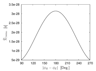
Figure 1: Extra time delay $\bar{\cal T}_{\rm Cosmo}$ measured in the proper time of observer on the Earth.

Figure 1 shows the estimated extra time delay $\bar{\cal T}_{\rm Cosmo}$ in the proper time of observer. The figure is plotted as the function of relative angle between the Mars $\phi_{R}$ and the Earth $\phi_{E}$, $|\phi_{R}-\phi_{E}|$ for $|\phi_{R}-\phi_{E}|>\pi/2$. The order of $\bar{\cal T}_{\rm Cosmo}$ is at most about $3.2\times 10^{-28}$ [s] which is considered as the typical magnitude of $\bar{\cal T}_{\rm Cosmo}$ for the planetary radar and the spacecraft ranging. Here let us evaluated the order of magnitude of each part in (18); the leading terms $H^{2}_{0}r^{3}/c^{3}\sim 10^{-28}$, the coupling terms $GMH^{2}_{0}r^{2}/c^{5}\sim v^{2}H^{2}_{0}r^{3}/c^{5}\sim 10^{-36}$, and $H^{4}_{0}r^{5}/c^{5}\sim 10^{-57}$ where we took $r_{E},v_{E}$ of Earth as $r,v$. However, it is much smaller than the current measurement limit, that is, the internal error of atomic clocks, $10^{-9}$ [s].

Next, we calculate (23) presuming again the Earth moving along the circular orbit, $r_{E}=1.5\times 10^{11}~{}[{\rm m}]$. The difference between the coordinate time and the proper one caused by the cosmological expansion is, in the interval of 100 [yr],

$$\tau_{\rm Cosmo}=-\frac{H_{0}^{2}r_{E}^{2}}{2c^{2}}(t-t_{0})\sim-4.1\times 10^{-20}~{}~{}{\rm[s]}.$$ (26)

This is also much smaller than the relative error of atomic clocks, $10^{-9}$ [s]. $\tau_{\rm Cosmo}$ causes the apparent orbital variations of longitude $\phi$ of planet, but it is $\delta\phi=n_{0}\tau_{\rm Cosmo}\sim-8.2\times 10^{-27}$ [rad] where $n_{0}=\sqrt{GM/r_{E}^{3}}\sim 2.0\times 10^{-7}$ [rad/s] is the mean motion of Earth. Then $\tau_{\rm Cosmo}$ does not has much effect on the observed $d{\rm AU}/dt$. Rounding up the results, the effect of cosmological expansion on the light propagation dose not give the explanation of observed increase of AU in the current solar system experiments.

Here we mention the attempts of Krasinsky and Brumberg (2004). They also investigated the secular increase of AU in terms of cosmological expansion deriving the approximate metric of Einstein equation, (5) of [25] which is the modified version of the standard form of Robertson-McVittie metric (1). In such a comoving form, they examined both the planetary motion and light propagation, then found there exist the large orbital variations in the radial and longitudinal directions due to the cosmological expansion ((19) and (20) of [25], respectively). However, these dynamical perturbations are completely canceled out by the time transformation between the coordinate time and proper one relating with light/signal propagation ((22) and (23) of [25], respectively). Hence they concluded that the cosmological effect cannot account for the observed $d{\rm AU}/dt$.

Before closing this section, we shortly note the dynamical effect due to the cosmological terms in the planetary motion. This problem has been studied by many authors [27, 14, 15, 16, 5, 6, 36, 30, 12, 4, 3, 19, 38, 10, 26]. And they showed that the cosmological influence on the planetary dynamics, e.g. the additional perihelion advance, is negligible small. We also confirmed that the cosmological terms are too small to give an account of the increasing of AU. In appendix A, we briefly summarize the results of the cosmological effect on the planetary motion based on (7).

6 Summary

In this paper, we investigated the light propagation passing near the gravitating body as the Sun embedded in the cosmological spacetime by means of the Robertson-McVittie solution. We concentrated on the time delay and derived the correction terms with respect to the Shapiro’s formula. We also took account of the time transformations; coordinate time to proper one, and conversely, proper time to coordinate one. These treatments are of importance when dealing with the observed round-trip time and its reduction process.

As the application of results, we considered the problem of increase of astronomical unit reported by Krasinsky and Brumberg (2004), since the AU is currently derived from the analysis of the round-trip time of light/signal. However, the effect of the cosmological expansion is too small to produce the observed $d{\rm AU}/dt=15$ [m/century] and then it dose not give the explanation of increase of AU.

Here it is worth to mention the interpretation of $d{\rm AU}/dt$. Although we and Krasinsky and Brumberg (2004) investigated the secular increasing of astronomical unit in terms of the cosmological effect, another possibility is suggested, that is, increasing of AU is arisen due to the lack of the calibrations of internal delays of the radio signals within the spacecrafts and this may be the most plausible reason of observed $d{\rm AU}/dt$. Nonetheless, till now, the origin of $d{\rm AU}/dt$ is far from clear therefore this issue should be explored by means of the every possibility we can imagine. And the re-analysis of $d{\rm AU}/dt$ using new data sets is also expected.

As we mentioned in the end of section 5, so far, the dynamical terms due to cosmological expansion in the planetary dynamics has been studied actively, while the influence on light/signal propagation has hardly been examined. However, the accuracy of astronomical/astrophysical observations, especially the optical, radio and arrival time ones, rapidly increases in the solar system and they may make it necessary to incorporate the cosmological effect in the future date. For this purpose, our investigation in present paper is the first attempt to this direction. To consider this problem, the matching of BCRS and cosmological reference system discussed by [19, 21] is also important issue to be investigated.

(7) expresses the completely static gravitational field, and is equivalent to Schwarzschild-de Sitter model. Nevertheless, as long as we focus on the solar system experiments, our results may be regarded as the dominant effects due to the cosmological expansion, see in (6). However in order to study the cosmological influence on the light/signal propagation in more detail and general cases, we must treat $H(t)$ and/or $a(t)$ as a function of time and adopt the time dependent spacetime model. This subject will be investigated at some future time.

We would like to express our gratitude to the referee for fruitful comments and suggestions. We acknowledge to G. A. Krasinsky for providing the information and comments about the AU issue. We also appreciate T. Fukushima, M. Kasai, H. Asada, Y. Itoh and M. Takada for fruitful discussions and comments. This work was partially supported by the Ministry of Education, Science, Sports and Culture, Grant-in-Aid, 18740165.

Appendix A Planetary Motion Based on Metric (7)

Cosmological influence on the planetary motion has studied by many authors as we mentioned in section 5. Then, in this appendix we limit to summarize our results based on (7) briefly.

The equation of motion in the quasi-Newtonian form becomes,

$$\frac{d^{2}r}{dt^{2}}-r\left(\frac{d\phi}{dt}\right)^{2}+\frac{GM}{r^{2}}=H_{0}^{2}r,\quad\frac{d}{dt}\left(r^{2}\frac{d\phi}{dt}\right)=0.$$ (27)

Supposing initially circular orbit $r=r_{0}=\mbox{const.}$, the mean motion is expressed as,

$$n=\frac{d\phi}{dt}\simeq n_{0}+\delta n,\quad\delta n=-n_{0}\frac{r_{0}^{3}H_{0}^{2}}{2GM}\sim 1.0\times 10^{-28}~{}~{}{\rm[rad/s]},$$ (28)

where $n_{0}=\sqrt{GM/r_{0}^{3}}\sim 2.0\times 10^{-7}$ [rad/s] and we took the orbital radius of Earth $r_{E}$ as $r_{0}$. From (28) the variation of longitude $\phi$ is evaluated in 100 [yr] as,

$$\delta\phi=\delta n(t-t_{0})\sim-3.5\times 10^{-18}~{}~{}{\rm[rad]}.$$ (29)

Also using (28), the orbital period of planet (in this case that of Earth) is written as,

$$T=\frac{2\pi}{n}\simeq T_{0}+\delta T,\quad\delta T=T_{0}\frac{r_{0}^{3}H_{0}^{2}}{2GM}\sim 7\times 10^{-26}~{}~{}{\rm[s]},$$ (30)

here $T_{0}=2\pi/n_{0}$. Finally putting $r=r_{0}+\delta r$ and inserting into (27), it yields,

$$\delta r=\frac{r_{0}^{4}H_{0}^{2}}{GM}\left(1+\frac{r_{0}^{3}H_{0}^{2}}{GM}\right)\sim 2.0\times 10^{-11}~{}~{}[{\rm m}].$$ (31)

Therefore we find that the estimated orbital variations $\delta r,\delta\phi$ and change of orbital period $\delta T$ are much smaller than the observed $d{\rm AU}/dt=15$ [m/century].

References

- Asada [2008] Asada, H., Phys. Lett. B, 661, 78 (2008).
- Bretagnon and Francou [1988] Bretagnon, P. and Francou, G., A&A, 202, 309 (1988).
- Carrera and Giulini [2005] Carrera, M. and Giulini, D., arXiv:gr-qc/0602098, (2005).
- Cooperstock et al. [1998] Cooperstock, F. I., Faraoni, V., and Vollick, D. N., ApJ, 503, 61 (1998).
- Einstein and Straus [1945] Einstein, A., and Straus, E. G. Rev. Mod. Phys., 17, 120 (1945).
- Einstein and Straus [1946] Einstein, A., and Straus, E. G., Rev. Mod. Phys., 18, 148 (1945).
- de Felice et al. [2004] de Felice, F., Crosta, M. T., Vecchiato, A., Lattanzi, M. G. and Bucciarelli, B., ApJ, 607, 580 (2004).
- de Felice et al. [2006] de Felice, F., Vecchiato, A., Crosta, M. T., Bucciarelli, B. and Lattanzi, M. G., ApJ, 653, 1552 (2006).
- Fairhead and Bretagnon [1990] Fairhead, L. and Bretagnon, P., A&A, 229, 240 (1990).
- Faraoni and Jacques [2007] Faraoni, V., and Jacques, A., Phys. Rev. D, 76, 3510 (2007).
- Fienga et al. [2008] Fienga, A., Manche, M., Laskar, J. and Gastineau, M., A&A, 477, 315 (2008).
- Gautreau [1984] Gautreau, R., Phys. Rev. D, 29, 198 (1984).
- Hellings [1986] Hellings, R. W., AJ, 91, 650 (1986).
- Järnefelt [1940a] Järnefelt, G., Ann. Acad. Soc. Sci. Fennicae, A45, 3 (1940).
- Järnefelt [1940b] Järnefelt, G., Arkiv Matem. Astron. Fys,, 27, 1 (1940).
- Järnefelt [1942] Järnefelt, G., Ann. Acad. Soc. Sci. Fennicae, A45, 12 (1942).
- Klioner [2003] Klioner, S. A., A&A, 404, 783 (2003).
- Klioner and Peip [2003] Klioner, S. A. and Peip, M., A&A, 410, 1063 (2003).
- Klioner and Soffel [2004] Klioner, S. A. and Soffel, M. H., Proc. of the Symposium ”The Three-Dimensional Universe with Gaia”, 305 (2004).
- Kopeikin [1997] Kopeikin, S. M., J. Math. Phys., 38, 2587 (1997).
- Kopeikin [2007] Kopeikin, S. M., AIP Conference Proc. “NEW TRENDS IN ASTRODYNAMICS AND APPLICATIONS III”, 886, 268 (2007).
- Kopeikin and Schäfer [1999] Kopeikin, S. M. and Schäfer, G., Phys. Rev. D, 60, 124002 (1999).
- Kopeikin and Mashhoon [2002] Kopeikin, S. M. and Mashhoon, B., Phys. Rev. D, 65, 64025 (2002).
- Krasinsky [2007] Krasinsky, G. A., Private Communications, (2007).
- Krasinsky and Brumberg [2004] Krasinsky, G. A. and Brumberg, V. A., Celest. Mech. Dyn. Astrn., 90, 267 (2004).
- Mashhoon et al. [2007] Mashhoon, B., Mobed, N., and Singh, D., Class. Quant. Grav., 24, 5031 (2007).
- McVittie [1933] McVittie, G. C., MNRAS, 93, 325 (1933).
- Moyer [1981a] Moyer, T. D., Celest. Mech., 23, 33 (1981).
- Moyer [1981b] Moyer, T. D., Celest. Mech., 23, 57 (1981).
- Noerdlinger and Petrosian [1971] Noerdlinger, P. D., and Petrosian, V., ApJ, 168, 1 (1971).
- Nolan [1999a] Nolan, B. C., Class. Quant. Grav., 16, 1227 (1999).
- Nolan [1999b] Nolan, B. C., Class. Quant. Grav., 16, 3183 (1999).
- Pijteva [2005] Pitjeva, E. V., Solar System Research, 39, 176 (2005).
- Richter and Matzner [1983] Richter, G.W. and Matzner, R. A., Phys. Rev. D, 28, 3007 (1983).
- Robertson [1928] Robertson, H. P., Phil. Mag., 7, 845 (1928).
- Schücking [1954] Schücking, E., Zeitschrift für Physik, 137, 595 (1954).
- Seidelmannn [2005] Seidelmann, P. K. (EDT), Explanatory Supplement to the Astronomical Almanac (Univ. Science Book, Sausalito, 2005).
- Sereno and Jetzer [2007] Sereno, M., and Jetzer, P., Phys. Rev. D, 75, 4031 (2007).
- Shapiro [1964] Shapiro, I. I., Phys. Rev. lett., 13, 789 (1964).
- Soffel et al. [2003] Soffel, M. H., Klioner, S. A., Petit, G., Wolf, P., Kopeikin, S. M., Bretagnon, P., Brumberg, V. A., Capitaine, N., Damour, T., Fukushima, T., Guinot, B., Huang, T.-Y., Lindegren, L., Ma, C., Nordtvedt, K., Ries, J. C., Seidelmann, P. K., Vokrouhlický, D., Will, C. M. and Xu, C., AJ, 126, 2687 (2003).
- Standish [2003] Standish, E. M., JPL Interoffice Memorandum, 312N, 03 (2003).
- Standish [2005] Standish, E. M., Proc. IAU Colloq., 196, 163 (2005).
- Will [1993] Will, C. M., Theory and experiment in gravitational physics (Cambridge Univ. Press, Cambridge, 1993).
- Will [2006] Will, C. M., Living Reviews in Relativity, http://relativity.livingreviews.org/Articles/lrr-2006-3/, (2006).