Formation and Transformation of Vector-Solitons in Two-Species Bose-Einstein Condensates with Tunable Interaction

Abstract

Under a unified theory we investigate the formation of various types of vector-solitons in two-species Bose-Einstein condensates with arbitrary scattering lengths. We then show that by tuning the interaction parameter via Feshbach resonance, transformation between different types of vector solitons is possible. Our results open up new ways in the quantum control of multi-species Bose-Einstein condensates.

Since the first realization of Bose-Einstein condensate (BEC), a tremendous amount of research has taken place in this interdisciplinary field first_experiment1 ; book . One specific topic of wide interest is multi-component BECs, which possess complicated quantum phases AlonPRL and properties not seen in individual components. Theoretical hoshenoy ; esry ; PuHPRL881130 and experimental cornell ; ModugnoScience294 ; hall studies have shown that inter-species interaction plays crucial roles in these systems. Recently, two-species BECs with tunable interaction Italy_twospecies ; Italy_twospecies1 were successfully produced . This important progress motivates further explorations of two-species BECs.

Solitons represent a highly nonlinear wave phenomenon with unique propagation features and have attracted great interests from many different fields, e.g., nonlinear optics opt . Because the nonlinear Schrödinger equation governing matter-wave solitons book ; darkexp ; Science2961290 ; nature is similar to those for solitons in other contexts, well-established understandings of solitons can be applied to atomic BECs to achieve better control of matter waves. However, BEC systems possess many unique features of their own and make it possible to study soliton phenomena under circumstances that cannot be easily realized in other fields.

In this paper, we provide a unified theory to investigate various types of vector solitons in two-species condensates with arbitrary scattering lengths. Remarkably, we find that by tuning the inter-species interaction via the well-established Feshbach resonance technique Italy_twospecies , different types of vector-solitons can be realized and even transformed to each other. In addition, these vector solitons can be dynamically stable in the presence of soft trapping potentials. Our theoretical work opens up new possibilities in the quantum control of multi-species BECs and other related complex systems.

The mean-field dynamics of a two-species BEC is governed by the following equations hoshenoy ; esry ; PuHPRL881130 ; book :

$$i\hbar\frac{\partial\psi_{1}}{\partial t}=[-\frac{\hbar^{2}\nabla^{2}}{2m_{1}}+V_{1}+U_{11}|\psi_{1}|^{2}+U_{12}|\psi_{2}|^{2}]\psi_{1},$$

$$i\hbar\frac{\partial\psi_{2}}{\partial t}=[-\frac{\hbar^{2}\nabla^{2}}{2m_{2}}+V_{2}+U_{21}|\psi_{1}|^{2}+U_{22}|\psi_{2}|^{2}]\psi_{2},$$

where the condensate wave functions are normalized by particle numbers $N_{i}\equiv\int|\psi_{i}|^{2}d^{3}{\bf r}$, $U_{ii}=4\pi\hbar^{2}a_{ii}/m_{i}$ and $U_{12}=U_{21}=2\pi\hbar^{2}a_{12}/m$ represent intra- and inter-species interaction strengths respectively, with $a_{ij}$ being the corresponding scattering lengths and $m$ the reduced mass. The trapping potentials are assumed to be $V_{i}=m_{i}[\omega_{ix}^{2}x^{2}+\omega_{i\perp}^{2}(y^{2}+z^{2})]/2$. Further assuming $\omega_{i\perp}\gg\omega_{ix}$ such that the transverse motion of the condensates are frozen to the ground state of the transverse harmonic trapping potential, the system becomes quasi-one-dimensional. Integrating out the transverse coordinates, the resulting equations for the axial wave functions $\tilde{\psi}_{1,2}(x)$ in dimensionless form can be written as

$$i\frac{\partial\tilde{\psi}_{1}}{\partial t}\!\! = \!\![-\frac{1}{2}\frac{\partial^{2}}{\partial x^{2}}+\frac{\lambda_{1}^{2}}{2}x^{2}+b_{11}|\tilde{\psi}_{1}|^{2}+b_{12}|\tilde{\psi}_{2}|^{2}]\tilde{\psi}_{1},$$ (1)

$$i\frac{\partial\tilde{\psi}_{2}}{\partial t}\!\! = \!\![-\frac{\kappa}{2}\frac{\partial^{2}}{\partial x^{2}}+\frac{\lambda_{2}^{2}}{2\kappa}x^{2}+b_{21}|\tilde{\psi}_{1}|^{2}+b_{22}|\tilde{\psi}_{2}|^{2}]\tilde{\psi}_{2},$$ (2)

where we have chosen $\sqrt{\hbar/(m_{1}\omega_{1\perp})}$ and $2\pi/\omega_{1\perp}$ to be the units for length and time, respectively; and $\tilde{\psi}_{1,2}$ is normalized such that $\int|\tilde{\psi}_{1}|^{2}dx=1$ and $\int|\tilde{\psi}_{2}|^{2}dx=N_{2}/N_{1}$. Other parameters in Eqs.  (1) and (2) are defined as: $b_{11}=2a_{11}N_{1}$, $b_{12}=b_{21}=2m_{1}a_{12}N_{1}/[(1+\gamma)m]$, $b_{22}=2a_{22}m_{1}N_{1}\gamma/m_{2}$, $\gamma=\omega_{2\perp}/\omega_{1\perp}$, $\lambda_{1}=\omega_{1x}/\omega_{1\perp}$, $\lambda_{2}=\omega_{2x}/\omega_{1\perp}$, and $\kappa=m_{1}/m_{2}$.

A unified treatment of different vector-soliton solutions – When the longitudinal trapping potential is neglected ($\lambda_{i}=0$), Eqs. (1) and (2) are perfectly integrable under the condition $\kappa=1$ (i.e., $m_{1}=m_{2}$) and $b_{11}=b_{12}=b_{21}=b_{22}$ int , allowing for a general procedure to construct two-component vector-soliton solutions in the form of “dark-dark” PRE554773 , “bright-dark” PRL87010401 and “bright-bright” solitons PRA48599 . When integrability is destroyed, previous studies show that distorted versions of soliton solutions exist, but closed form can only be given for special cases and often for one particular type of vector soliton special . Here we show that, even when the above-mentioned integrability condition is violated (e.g., for arbitrary interaction strengths $b_{ij}$ and mass ratio $\kappa$), there still exists in general a specific class of exact solutions that include all types of vector solitons, so long as $b_{12}^{2}\neq b_{11}b_{22}$. The type of vector soliton is determined by the values of $b_{ij}$ and $\kappa$.

The vector-soliton solution can be found by inserting an appropriate ansatz (see below) into Eqs.  (1) and (2). Defining the following two quantities:

$$C_{1} \equiv (b_{22}-\kappa b_{12})/(b^{2}_{12}-b_{11}b_{22})\,,$$

$$C_{2} \equiv (b_{12}-\kappa b_{11})/(b^{2}_{12}-b_{11}b_{22})\,,$$

the conditions under which various vector-soliton solutions exist are found to be:

$$C_{1}>0,\,C_{2}<0:\;\;{\rm bright-bright}\;({\rm BB}),$$

$$C_{1}>0,\,C_{2}>0:\;\;{\rm bright-dark}\;({\rm BD}),$$

$$C_{1}<0,\,C_{2}>0:\;\;{\rm dark-dark}\;({\rm DD}),$$

$$C_{1}<0,\,C_{2}<0:\;\;{\rm dark-bright}\;({\rm DB}).$$

Explicit expressions for these vector-solitons are then found from the ansatz we use. In particular, the BB solution (i.e., bright soliton for species 1 and bright soliton for species 2; analogous convention applies to all other solutions) is given by

$$\tilde{\psi}_{1B}\!\! =\!\! \eta\sqrt{C_{1}}\,{\rm sech}(\eta x-\eta vt)\,e^{i\left[vx+\left({\eta^{2}}-{v^{2}}\right)t/2\right]}\,,$$

$$\tilde{\psi}_{2B}\!\! =\!\! \eta\sqrt{-C_{2}}\,{\rm sech}(\eta x-\eta vt)\,e^{i\left[{v}x/{\kappa}+\left({\kappa}\eta^{2}-v^{2}/\kappa\right)t/2\right]}.$$

The BD solution is given by

$$\tilde{\psi}_{1B}\!\! =\!\! \eta\sqrt{C_{1}}\,{\rm sech}(\eta x-\eta vt)\,e^{i\left[vx+f_{1}t\right]}\,,$$ (3a)

$$\tilde{\psi}_{2D}\!\! = \!\![iv\sqrt{C_{2}}/\kappa+\eta\sqrt{C_{2}}\,\tanh(\eta x\!\!-\!\!\eta vt)]e^{if_{2}t},$$ (3b)

with $f_{1}=\left({\eta^{2}}-{v^{2}}\right)/2-b_{12}C_{2}(\eta^{2}+v^{2}/\kappa^{2})$ and $f_{2}=-b_{22}C_{2}(\eta^{2}+v^{2}/\kappa^{2})$. The DD solution is found to be

$$\tilde{\psi}_{1D}\!\! = \!\![iv\sqrt{-C_{1}}+\eta\sqrt{-C_{1}}\,\tanh(\eta x-\eta vt)]\,e^{if_{1}t}\,,$$

$$\tilde{\psi}_{2D}\!\! = \!\![iv\sqrt{C_{2}}/\kappa+\eta\sqrt{C_{2}}\,\tanh(\eta x-\eta vt)]\,e^{if_{2}t}\,,$$

with $f_{1}=-\eta^{2}-v^{2}(-b_{11}C_{1}+b_{12}C_{2}/\mu^{2})$ and $f_{2}=-\mu\eta^{2}-v^{2}(-b_{21}C_{1}+b_{22}C_{2}/\mu^{2})$. Finally, the DB solution can be obtained from the BD solution (3) by exchanging indices 1 and 2, and let $C_{1,2}\rightarrow-C_{1,2}$. In all these cases, the parameter $\eta$ determines the width of the soliton and can be found by the normalization condition for $\tilde{\psi}_{1,2}$. The parameter $v$ gives the velocity of the soliton. We note that the BB solution under the condition $b_{11},b_{22}>0$ and $b_{12}<0$, but not the other cases, has been studied by Pérez-García and Beitia pra . The exact expressions for vector solitons found here bear an apparent resemblance to those for integrable systems int .

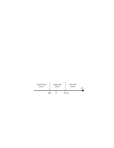
Figure 1: Phase diagram of vector solitons vs. inter-species interaction $b_{12}$ for the system with $b_{11}<0$ and $b_{22}>0$. As described in the text, the unit of $b_{ij}$ is $\sqrt{\hbar/(m_{1}\omega_{1\perp})}$. In the examples shown later in the paper, the two species experience the same trapping frequency: $\omega_{1\perp}=\omega_{2\perp}=2\pi\times 710$Hz. The number of atoms in the first species (⁷Li) is assumed to be 5000, which results in the dimensionless intra-species interaction strength $b_{11}=-1.47$ and $b_{22}=5.89$. The two critical values of the inter-species interaction strength are therefore $\kappa b_{11}=-0.45$ and $b_{22}/\kappa=19.35$.

Dynamics and dynamical stability – To be specific, we take ⁷Li as species 1 and ²³Na as species 2, with fixed and realistic intra-species interaction strength $b_{11}<0$, $b_{22}>0$ and variable inter-species interaction strength $b_{12}$. Figure  1 depicts the “phase diagram” for different regimes of vector solitons as $b_{12}$ is varied. As is indicated in Fig.  1, the system supports BB ($b_{12}<\kappa b_{11}$), BD ($\kappa b_{11}<b_{12}<b_{22}/\kappa$) and DD ($b_{12}>b_{22}/\kappa$) vector soliton, while the condition for DB soliton can never be satisfied for this particular ⁷Li–²³Na system.

To study the dynamical stability of the vector-soliton solutions given above, we first calculate the collective excitation frequencies by solving the corresponding Bogoliubov-de Gennes equation PuHPRL881130 . Our calculations show that, the excitation frequencies of the BB and BD vector-solitons are all real, while those of the DD vector-soliton contain complex values. We hence conclude that, for the ⁷Li-²³Na system, the BB and BD vector-solitons are dynamically stable, while the DD vector-soliton is dynamically unstable.

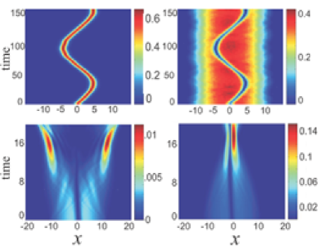
Figure 2: (Color online) Dynamics of vector solitons inside a weak longitudinal trap with $\lambda_{1}=\lambda_{2}=0.1$. Other parameters are specified in Fig. 1. Units for $x$ and time are $\sqrt{\hbar/(m_{1}\omega_{1\perp})}$ and $2\pi/\omega_{1\perp}$. The left and right plots represent the longitudinal density profiles of the first and second species, respectively. Upper panel: evolution of a BD vector soliton with $b_{12}=2$ initially located at $x=0$ and velocity $v=0.1$. Lower panel: evolution of a DD vector soliton with $b_{12}=30$. For the system under study, the BD (DD) vector soliton is dynamically stable (unstable).

This stability analysis is confirmed by direct numerical simulations of Eqs. (1) and (2). Computational examples are shown in Fig. 2. In our simulation, a harmonic trapping potential is added along the longitudinal direction to represent a more realistic situation. The trapping potential is weak such that its variation across the soliton scale is negligible. Such a soft trapping potential spatially confines the solitons without affecting their essential properties. The upper panel of Fig. 2 shows the evolution of a BD vector soliton. For the initial condition, we use the exact solution of Eq. (3a) for the bright component, while in order to confine the dark soliton inside the trap, we multiply Eq. (3b) by a Thomas-Fermi profile with an inverted parabolic shape to simulate the dark component which is a quite standard practice PRL87010401 . The presence of the weak longitudinal trap causes the vector soliton to oscillate while maintaining the overall shape as shown in the upper panel of Fig. 2. By contrast, the lower panel of Fig. 2 shows that the DD soliton is dynamically unstable — an initial DD vector-soliton is quickly destroyed and the two species tend to phase separate into different spatial regions due to the large inter-species repulsion. We remark that there exist alternative ways to study the soliton dynamics, for example, the variational approach used in Ref. LiH .

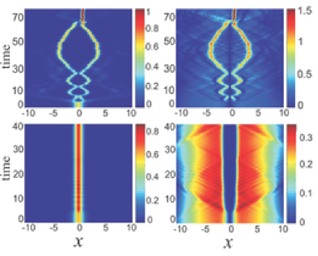
Figure 3: (Color online) Conversion between different types of vector solitons via Feshbach resonance. The left and right plots represent the longitudinal density profiles of the first and second species, respectively. Units for $x$ and time are $\sqrt{\hbar/(m_{1}\omega_{1\perp})}$ and $2\pi/\omega_{1\perp}$. Initially, a BD vector soliton is prepared with $b_{12}=2$. Other parameters are the same as in Fig. 2. Upper panel: From $t=3$ to 4, $b_{12}$ is linearly varied to a final value of $-10$ and stays at that value afterwards. Lower panel: From $t=3$ to 23, $b_{12}$ is linearly varied to a final value of 30 and stays at that value afterwards.

Soliton transformation via Feshbach resonance – Controlling the interaction strength via Feshbach resonace is a unique possibility afforded by atomic systems. Fig. 3 shows an example of dynamical conversion between different types of vector solitons via an inter-species Feshbach resonance. Initially, we prepare a zero-velocity BD vector soliton by choosing a proper $b_{12}$ whose value is tuned in later time. In the upper panel of Fig. 3, $b_{12}$ is changed to a value less than $\kappa b_{11}$. For this new value of $b_{12}$, the system supports BB, but not BD, vector solitons (see Fig. 1). The upper panel of Fig. 3 shows that the initial BD vector soliton is indeed destroyed after $b_{12}$ is changed to the new value. The system first evolves into two pairs of BB vector-solitons with finite relative velocity. These two pairs go through several collisions and eventually merge into one single pair. During the evolution, significant radiation from the second species is observed. According to the exact BB solution given above, the number of atoms in each species satisfy

$$\frac{N_{1}}{N_{2}}=\frac{C_{1}}{-C_{2}}=\frac{b_{22}-\kappa b_{12}}{\kappa b_{11}-b_{12}}\,.$$

Using realistic values of $b_{11}$ and $b_{22}$ (as detailed in the caption of Fig. 1), we have $N_{1}/N_{2}=0.935$. Numerically, we found this ratio to be $0.92\sim 0.95$ which is in good agreement with the theoretical value. It is simple to check and intuitive to understand that when the initial BD vector-soliton breaks into two pairs of BB solitons, the relative phase of the two bright solitons of the first species is zero, while that of the second species is $\pi$. Just like in the scalar condensate case, this leads to attractive (repulsive) soliton-soliton interaction within the first (second) species. We also remark that the relative velocity of the BB vector-soliton pairs thus generated is sensitive to how fast $b_{12}$ is varied. In general, the faster $b_{12}$ is varied, the larger the relative velocity. If we vary $b_{12}$ much slower, the pairs (with smaller relative velocity) will merge together later and experience more collisions. This observation suggests that varying the sweeping rate of $b_{12}$ should help understand more about the collision dynamics of multiple BB vector-soliton pairs  pra ; last .

In the example shown in the lower panel of Fig. 3, $b_{12}$ is changed to a value larger than $b_{22}/\kappa$, i.e., into the DD vector-soliton regime. Here the BD vector soliton does not evolve into a DD vector soliton, which is consistent with the fact that the DD solution is unstable. Instead, due to the strong inter-species repulsion, the core region of the initial dark soliton of species 2 is widened, and is no longer accurately described by a tanh function. In the mean time, the bright soliton of species 1 is narrowed and remain captivated inside the core of the dark component. This property may help to produce and stabilize bright solitons. During the evolution, we can also see that additional dark solitons can be generated from the core region of species 2 (see the lower right figure in Fig. 3). Of particular interest are those new dark solitons generated at early times: They move away from the core, then get bounced back by the trapping potential, and finally get reflected by the central BD vector soliton. Recently similar behavior — the reflection of dark soliton by a BD vector soliton — was observed experimentally nature .

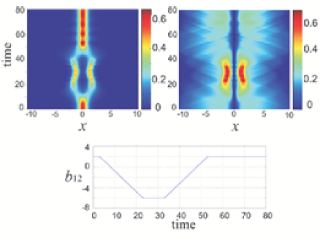
Figure 4: (Color online) Conversion between BB and BD vector solitons. The left and right plots of the upper panel represent the longitudinal density profiles of the first and second species, respectively. The lower panel shows the variation of $b_{12}$. Unit for $x$ and $b_{12}$ is $\sqrt{\hbar/(m_{1}\omega_{1\perp})}$, and unit for time is $2\pi/\omega_{1\perp}$. Initially, a BD vector soliton is prepared with $b_{12}=2$. Other parameters are the same as in Fig. 2.

Figure  4 illustrates another example of the conversion between different types of vector-solitons via inter-species Feshbach resonance. The initial condition is the same as in Fig. 3 where a zero-velocity BD vector-soliton is prepared. The value of $b_{12}$ is then decreased and the system evolves to two BB vector-soliton pairs as in Fig. 3. Then, we restore the initial value of $b_{12}$ before the two BB vector-solitons merge into one. As seen in Fig. 4, such a controlled tuning of $b_{12}$ can also recover the initial BD vector-soliton. This represents a remarkable example of the coherent control over the BEC dynamics, afforded by the tunability of interaction strength.

In conclusion, we put forward a unified theory to treat all types of vector solitons on equal footing in two-species BECs with arbitrary scattering length. More importantly, we show that different types of vector solitons can be transformed to each other by varying the interaction strength. Besides its fundamental interest in quantum dynamics, our study may also find applications in the quantum control of multi-species BECs. For example, treating one atomic species as the target, its soliton properties can be controlled by the presence of a second species via the tuning of the interaction strength between them. We hope that these results can stimulate investigation of novel phenomena in nonlinear complex systems in general and further studies of BEC solitons in particular.

XXL was partially supported by the International Collaboration Fund, National Univ. of Singapore. JG is supported by the start-up fund (WBS grant No. R-144-050-193-101/133) and the “YIA” fund (WBS grant No. R-144-000-195-123) from the National Univ. of Singapore. HP acknowledges support from the NSF of US and the Welch Foundation (Grant No. C-1669). WML is supported by the NSF of China under Grant Nos. 10874235, 60525417, 10740420252, the NKBRSF of China under Grant 2005CB724508, 2006CB921400.

References

- (1) M. H. Anderson et al., Science 269, 198 (1995); K. B. Davis et al., Phys. Rev. Lett. 75, 3969 (1995); C. C. Bradley, et al., Phys. Rev. Lett. 75, 1687 (1995).
- (2) P. G. Kevrekidis, D. J. Frantzeskakis and R. Carretero-González, ed. Emergent Nonlinear Phenomena in Bose-Einstein Condensates (Springer-Verlag, Berlin, 2008).
- (3) O. E. Alon et al., Phys. Rev. Lett. 95, 030405 (2005).
- (4) T. L. Ho et al., Phys. Rev. Lett. 77, 3276 (1996).
- (5) B. D. Esry et al., Phys. Rev. Lett. 78, 3594 (1997).
- (6) H. Pu and N. P. Bigelow, Phys. Rev. Lett. 80, 1130 (1998); ibid 80, 1134 (1998).
- (7) C. J. Myatt et al., Phys. Rev. Lett. 78, 586 (1997).
- (8) G. Modugno et al., Science 294, 1320 (2001).
- (9) D. S. Hall, in Ref. book .
- (10) G. Thalhammer et al., Phys. Rev. Lett. 100, 210402 (2008).
- (11) S. B. Papp et al., Phys. Rev. Lett. 101, 040402 (2008).
- (12) Yu. S. Kivshar and G. P. Agrawal, Optical Solitons: From Fibers to Photonic Crystals (Academic Press, San Diego, 2003).
- (13) S. Burger et al., Phys. Rev. Lett. 83, 5198 (1999); J. Denschlag et al., Science 287, 97 (2000).
- (14) K. E. Strecker et al., Nature 417, 150 (2002); L. Khaykovich et al., Science 296, 1290 (2002).
- (15) C. Becker et al., Nature Phys. 4, 496 (2008).
- (16) S. V. Manakov, Sov. Phys. JETP 38, 248 (1974); V. G. Makhankov et al., Phys. Lett. A 81, 161 (1981); T. Kanna et al., Phys. Lett. A 330, 224 (2004).
- (17) A. P. Sheppard and Y. S. Kivshar. Phys. Rev. E 55, 4773 (1997); V. A. Brazhnyi and V. V. Konotop. Phys. Rev. E 72, 026616 (2005).
- (18) Th. Busch and J. R. Anglin, Phys. Rev. Lett. 87, 010401 (2001).
- (19) D. J. Kaup and B. A. Malomed, Phys. Rev. A 48, 599 (1993); B. A. Malomed et al., Phys. Rev. E 58, 2564 (1998) .
- (20) P. G. Kevrekidis et al., Eur. Phys. J. D 28, 181 (2004); A. V. Buryak, Y. S. Kivshar, and D.F. Parker, Phys. Lett. A 215, 57 (1996).
- (21) V. M. Pérez-García and J. B. Beitia, Phys. Rev. A 72, 033620 (2005).
- (22) H. Li et al., Chaos, Solitons and Fractals, in press doi:10.1016/j.chaos.2007.06.063.
- (23) J. Babarro et al., Phys. Rev. A 71, 043608 (2005).