High-frequency corrections to the detector response and their effect on searches for gravitational waves

Abstract

Searches for gravitational waves with km-scale laser interferometers often involve the long-wavelength approximation to describe the detector response. The prevailing assumption is that the corrections to the detector response due to its finite size are small and the errors due to the long-wavelength approximation are negligible. Recently, however, Baskaran and Grishchuk (2004 Class. Quantum Grav. 21 4041) found that in a simple Michelson interferometer such errors can be as large as 10 percent. For more accurate analysis, these authors proposed to use a linear-frequency correction to the long-wavelength approximation. In this paper we revisit these calculations. We show that the linear-frequency correction is inadequate for certain locations in the sky and therefore accurate analysis requires taking into account the exact formula, commonly derived from the photon round-trip propagation time. Also, we extend the calculations to include the effect of Fabry-Perot resonators in the interferometer arms. Here we show that a simple approximation which combines the long-wavelength Michelson response with the single-pole approximation to the Fabry-Perot transfer function produces rather accurate results. In particular, the difference between the exact and the approximate formulae is at most 2-3 percent for those locations in the sky where the detector response is greater than half of its maximum value. We analyse the impact of such errors on detection sensitivity and parameter estimation in searches for periodic gravitational waves emitted by a known pulsar, and in searches for an isotropic stochastic gravitational-wave background. At frequencies up to 1 kHz, the effect of such errors is at most 1-2 percent. For higher frequencies, or if more accuracy is required, one should use the exact formula for the detector response.

, ,

1 Introduction

Searches for gravitational waves are currently conducted with km-scale laser interferometers such as LIGO [1] and VIRGO [2]. These detectors utilize a Michelson configuration which is further enhanced by the addition of Fabry-Perot cavities in the interferometer arms. Development of efficient data analysis algorithms requires accurate knowledge of the response of these detectors to gravitational waves. There are two somewhat different points of view on how to calculate the detector response. In one approach, it is assumed that the size of the detector is much less than the wavelength of the incoming gravitational wave, and therefore can be neglected in the calculations. This approach is often called the long-wavelength approximation [3, 4]. The advantage of this approximation is that it allows one to interpret the effect of gravitational waves entirely in terms of the motion of test masses, which is appealing to our physical intuition. In another approach, one takes into account the finite size of the detector by considering variations in the gravitational wave within the duration of one photon round trip between the test masses [5]-[10]. The detector response obtained in this way is more accurate but no longer allows the simple interpretation in terms of test mass motion [11]. Such calculations are commonly used to derive the response of space-borne gravitational-wave antennae [12]-[16]. For ground-based detectors, one usually adopts the long-wavelength approximation, assuming that it is sufficiently accurate.

It was pointed out by Baskaran and Grishchuk [17] that even for ground-based detectors, the long-wavelength approximation can lead to noticeable errors in the estimation of parameters of a gravitational wave. In particular, they found that the error in searches for periodic gravitational waves can be as large as 10%, thus raising a concern about the validity of the long-wavelength approximation in recent searches for gravitational waves. Some key points of their analysis however required clarification. The authors assumed that for ground-based detectors it suffices to use the first-order correction to the long-wavelength approximation and thus introduced a linear-frequency detector response, whereas the exact, non-linear formula was readily available. Also, the calculations did not take into account the presence of Fabry-Perot cavities in the interferometer arms, which play a crucial role in the formation of the signal. It is therefore worthwhile to reconsider this analysis.

In this paper we re-evaluate the errors due to the long-wavelength approximation and assess their impact on current searches for gravitational waves with km-scale laser interferometers. We show that the linear-frequency approximation is inadequate for some locations in the sky, and therefore one must use the exact formula for the detector response to estimate systematic errors from the long-wavelength approximation. To make the analysis applicable for LIGO and VIRGO detectors, we include the transfer function of Fabry-Perot cavities in the interferometer arms. Using the exact expression for the detector response, we estimate the errors resulting from the long-wavelength approximation in searches for periodic gravitational waves and in searches for an isotropic stochastic gravitational-wave background.

2 Michelson interferometer response (long-wavelength approximation)

In the transverse-traceless gauge [3], a plane gravitational wave coming from direction $\hat{n}$ on the sky is given by

$$h_{ij}(t,\vec{x})=h_{+}(t,\vec{x})\,e_{ij}^{+}(\hat{n})+h_{\times}(t,\vec{x})\,e_{ij}^{\times}(\hat{n})\,,$$ (1)

where $h_{+,\times}(t,\vec{x})=h_{+,\times}(t+\vec{x}\cdot\hat{n}/c)$, and the polarisation tensors are

$${e}^{+}_{ij}(\hat{n})={\ell}_{i}{\ell}_{j}-{m}_{i}{m}_{j},$$ (2)

$${e}^{\times}_{ij}(\hat{n})={\ell}_{i}{m}_{j}+{\ell}_{j}{m}_{i}\,.$$ (3)

The unit vectors $\hat{\ell}$ and $\hat{m}$ are chosen so that $\hat{\ell},\hat{m},\hat{n}$ form a right-handed orthonormal basis. The rotational degree of freedom associated with the choice of $\hat{\ell}$ and $\hat{m}$ in the plane perpendicular to $\hat{n}$ is often called the polarisation angle $\beta$. In what follows, we will suppress $\beta$-dependence for simplicity.

Consider a Michelson interferometer with arms aligned along the unit vectors $\hat{a}$ and $\hat{b}$. In the long-wavelength approximation, a signal produced by a gravitational wave in the detector [4, 18] is given by

$$V(t)=\frac{1}{2}(a^{i}a^{j}-b^{i}b^{j})h_{ij}(t,\vec{0})\,,$$ (4)

where we assumed that the detector is located at $\vec{x}=\vec{0}$ and its size is negligible. Equivalently, the signal can be written as

$$V(t)=F_{+}(\hat{n})h_{+}(t)+F_{\times}(\hat{n})h_{\times}(t)\,,$$ (5)

where

$$F_{A}(\hat{n})=\frac{1}{2}\,(a_{i}a_{j}-b_{i}b_{j}){e}_{A}^{ij}(\hat{n})$$ (6)

are the interferometer responses to the two independent polarisations $(A=+,\times)$ of the gravitational wave. In the frequency domain, (5) becomes

$$\tilde{V}(f)=F_{+}(\hat{n})\tilde{h}_{+}(f)+F_{\times}(\hat{n})\tilde{h}_{\times}(f)\,.$$ (7)

In what follows, tilde always denotes Fourier transform with respect to $t$.

Three-dimensional representations of the absolute value of $F_{A}$ as a function of $\hat{n}$ are often called antenna patterns. Antenna patterns have traditionally been shown for a particular choice of polarisation basis: $\hat{\ell}=\hat{\theta}$ and $\hat{m}=\hat{\phi}$, where $\hat{\theta}$ and $\hat{\phi}$ are the unit vectors corresponding to the spherical coordinates $\phi\in[0,360^{\circ}]$ and $\theta\in[0,180^{\circ}]$. Figure 1 shows the antenna patterns in the coordinate system with the $x$ and $y$ axes aligned with the interferometer arms. In these coordinates, $\hat{n}=(\sin\theta\cos\phi,\sin\theta\sin\phi,\cos\theta)$.

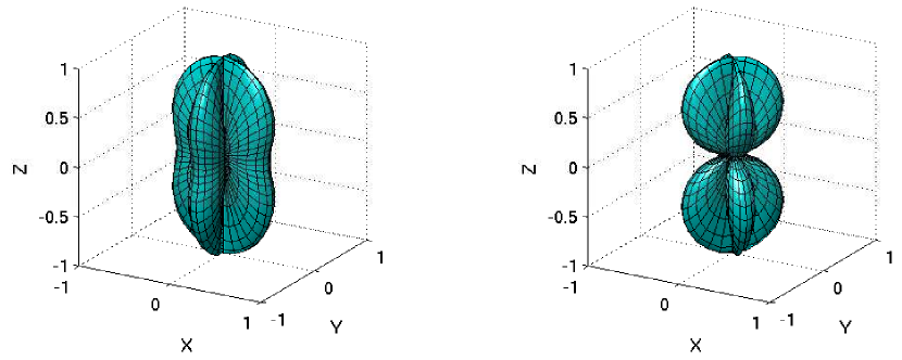
Figure 1: Antenna patterns in the long-wavelength approximation: $|F_{+}(\hat{n})|$ (left) and $|F_{\times}(\hat{n})|$ (right). They can also be obtained as the limiting case ($f=0$) of the exact response functions, described in section 3.2.

3 Michelson interferometer response (exact formula)

The detector response which takes into account the finite size of the interferometer will be called here exact in contrast to the approximate response (6). Here we give a brief derivation of the exact detector response following recent calculations in [19, 20].

3.1 Photon propagation time

The interval for photons propagating in spacetime with a gravitational wave (1) is

$$\rmd s^{2}=-c^{2}\rmd t^{2}+\left[\delta_{ij}+h_{ij}(t,\vec{x})\right]\rmd x^{i}\rmd x^{j}=0\,.$$ (8)

Consider a photon launched in the direction $\hat{a}$ to be bounced back by a mirror some distance $L$ away. On the way forward, the unperturbed photon trajectory is $x^{i}=a^{i}\xi$, where $\xi\in[0,L]$. Substituting this trajectory in (8) and solving for $t$, we obtain

$$c(t-t_{0})=\int_{0}^{\xi}\left(1+h_{ij}\,a^{i}a^{j}\right)^{1/2}\rmd\xi^{\prime}.$$ (9)

Let $T$ be the nominal (unperturbed) photon transit time: $T\equiv L/c$. In the presence of a gravitational wave, the transit time will slightly deviate from its nominal value giving rise to a small perturbation:

$$\delta T(t)=\frac{1}{2c}a^{i}a^{j}\int_{0}^{L}h_{ij}\left(t_{0}+\frac{\xi}{c}+\frac{\hat{n}\cdot\hat{a}}{c}\xi\right)\rmd\xi,$$ (10)

where $t_{0}$ is the starting time for the photon propagation which can be approximated by $t_{0}=t-T$. Similarly, on the way back,

$$\delta T^{\prime}(t)=\frac{1}{2c}a^{i}a^{j}\int_{0}^{L}h_{ij}\left(t_{0}+\frac{L-\xi}{c}+\frac{\hat{n}\cdot\hat{a}}{c}\xi\right)\rmd\xi,$$ (11)

where $t_{0}$ can also be approximated by $t_{0}=t-T$. Then the perturbation of the round-trip time is given by

$$\delta T_{\mathrm{r.t.}}(t)=\delta T(t-T)+\delta T^{\prime}(t).$$ (12)

In the Fourier domain, it can be written as

$$\frac{\delta\tilde{T}_{\mathrm{r.t.}}(f)}{T}=a_{i}a_{j}\,D(\hat{a},f)\,e^{ij}_{A}(\hat{n})\,\tilde{h}_{A}(f),$$ (13)

where we introduced the transfer function

$$D(\hat{a},f)=\frac{\rme^{-i2\pi fT}}{2}\,\left[\rme^{i\pi fT_{+}}{\mathrm{sinc}}\left(\pi fT_{-}\right)+\rme^{-i\pi fT_{-}}{\mathrm{sinc}}\left(\pi fT_{+}\right)\right],$$ (14)

with short-hand notation: $T_{\pm}\equiv T(1\pm\hat{a}\cdot\hat{n})$. Further calculations require switching from photons to continuous electro-magnetic waves.

3.2 Phase lag of a continuous electro-magnetic wave

Figure 2: Simple Michelson interferometer (left) and Michelson interferometer with Fabry-Perot arm cavities (right). Enlarged is a schematic picture of the photon trajectory in the $\hat{a}$ arm. (Forward and return paths are separated for clarity.) Here we neglected the recycling mirror which increases the power incident on the beam splitter but otherwise does not affect the detector response.

For an electro-magnetic wave propagating in the $\hat{a}$-direction, the electric field is given by $\mathcal{E}(t,\vec{x})=A\exp[i(\omega t-k\vec{x}\cdot\hat{a})]$, where $A$ is the amplitude, $\omega$ is the frequency, and $k$ is the wavenumber ($k=\omega/c$). It is convenient to suppress the fast-oscillating factor $\rme^{i\omega t}$ by introducing the slowly-varying amplitude [21]: $E=\mathcal{E}\rme^{-i\omega t}$. Consider a simple Michelson interferometer with equal arm lengths, $L$, as shown in figure 2 (left). The phase delay of the electro-magnetic field returning to the beam splitter after a round trip in the arm is $\omega(2T+\delta T_{\mathrm{r.t.}})=2kL+\psi$, where

$$\psi(t)=\omega\,\delta T_{\mathrm{r.t.}}(t)\,$$ (15)

is the phase delay due to the gravitational wave. Two such phases corresponding to arms $\hat{a}$ and $\hat{b}$ will be denoted here $\psi_{\hat{a}}$ and $\psi_{\hat{b}}$. Let the amplitude of the field immediately after the beam splitter be $A_{0}$. Then the amplitude of the field incident on the beam splitter from arm $\hat{a}$ is $E_{\hat{a}}=A_{0}\,\exp(-2ikL-i\psi_{\hat{a}})$, and similarly for $E_{\hat{b}}$. Assuming that the interferometer operates at the dark fringe (destructive interference), we find that the field at the output (signal) port is proportional to

$$E_{\hat{a}}(t)-E_{\hat{b}}(t)\approx-iA_{0}\,\rme^{-2ikL}[\psi_{\hat{a}}(t)-\psi_{\hat{b}}(t)]\,.$$ (16)

With appropriate normalization the signal is given by

$$V(t)=\frac{1}{2\omega T}[\psi_{\hat{a}}(t)-\psi_{\hat{b}}(t)]\,.$$ (17)

In the Fourier domain, it can be written as

$$\tilde{V}(f)=G_{+}(\hat{n},f)\tilde{h}_{+}(f)+G_{\times}(\hat{n},f)\tilde{h}_{\times}(f)\,,$$ (18)

where $G_{A}(\hat{n},f)$ are the exact detector responses to the two independent polarisations of the gravitational wave:

$$G_{A}(\hat{n},f)=\frac{1}{2}\left[a_{i}a_{j}\,D(\hat{a},f)-b_{i}b_{j}\,D(\hat{b},f)\right]e^{ij}_{A}(\hat{n})\,.$$ (19)

Note that the long-wavelength formula (6) is a special case of the exact response:

$$F_{A}(\hat{n})=G_{A}(\hat{n},0).$$ (20)

As the frequency of the gravitational wave increases, the difference between $F_{A}$ and $G_{A}$ becomes more and more pronounced [9, 22]. The most drastic change occurs at the inverse of the photon round-trip time: $f=1/(2T)$. In Fabry-Perot cavities this quantity is called the free spectral range or FSR (see section 4.1).

Figure 3 shows the magnitude of the detector response functions $G_{A}(\hat{n},f)$ at the free spectral range of the 4-km LIGO interferometers ($f=37.5$ kHz). Note the presence of additional lobes in the antenna patterns, and a factor of 5-8 reduction in magnitude compared to the response at $f=0$, shown in figure 1.

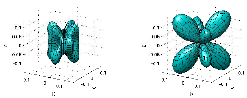
Figure 3: Antenna patterns at the FSR frequency (37.5 kHz): $|G_{+}(\hat{n},f)|$ (left) and $|G_{\times}(\hat{n},f)|$ (right).

3.3 Approximate formulae for the Michelson response

The long-wavelength approximation (6) is obtained by entirely neglecting the frequency dependence of the exact response

$$G_{A}(\hat{n},f)\approx F_{A}(\hat{n}).$$ (21)

A moderate frequency dependence is obtained by adding the first-order correction:

$$G_{A}(\hat{n},f)\approx F_{A}(\hat{n})+f\,\frac{\partial G_{A}}{\partial f}(\hat{n},0)\,.$$ (22)

This may not necessarily be a better approximation than (21) since the higher order terms neglected in (22) can be greater than the first-order term (proportional to first derivative). This happens because the first-order term vanishes at some locations in the sky whereas the sum of all higher order terms remains non-zero.

The most recent estimation of errors introduced by the long-wavelength approximation is due to Baskaran and Grishchuk [17]. These authors argued in favour of the linear approximation of the detector response (22), and estimated the corrections to the long-wavelength formula using the first-order ($f$-proportional) term. (In [17], the two terms in the right-hand side of (22) are called electric and magnetic components.) As we have shown, such a linear approximation is problematic. Fortunately, one need not be concerned with the accuracy of the linear approximation since the exact formula is readily available.

4 Transfer function of Fabry-Perot arm cavities

The response of LIGO and VIRGO detectors is enhanced by incorporation of optical resonators (Fabry-Perot cavities) in interferometer arms. Here we briefly derive the transfer function of a Fabry-Perot cavity and include it in the exact detector response.

4.1 Phase amplification due to multi-beam interference

Consider a Fabry-Perot cavity in one of the arms of the interferometer, as shown in figure 2 (right). Let the amplitude of the light incident on the cavity be $A_{0}$. Then the fields circulating in the cavity satisfy

$$E_{1}(t) = t_{1}A_{0}-r_{1}E_{2}(t),$$ (23)

$$E_{2}(t) = -r_{2}\,E_{1}(t-2T)\,\rme^{-2ikL-i\psi(t)},$$ (24)

where $t_{1}$ is the transmissivity of the front mirror, and $r_{1,2}$ are the reflectivities of the front and back mirror, respectively. Here $\psi$ is the phase lag due to the gravitational wave, (15). The condition for resonance implies that $L$ is equal to an integer number of half-wavelengths of light and therefore $\rme^{-2ikL}=1$.

The field returning to the beam splitter from the cavity, $E_{\hat{a}}=r_{1}A_{0}+t_{1}E_{2}$, consists of the promptly reflected field and the leakage field. The information about the gravitational wave is contained in the leakage field which is proportional to internal field $E_{2}$. Let the amplitude and the phase of this field be $A$ and $\Psi$, i.e. $E_{2}=A\rme^{-i\Psi}$. Solving equations (23) and (24) to first order in $\Psi$, we find that the amplitude is given by $A=-t_{1}r_{2}A_{0}/(1-r_{1}r_{2})$ and that the phase satisfies the equation

$$\Psi(t)-r_{1}r_{2}\Psi(t-2T)=\psi(t)\,,$$ (25)

or equivalently,

$$\Psi(t)=\sum_{k=0}^{\infty}(r_{1}r_{2})^{k}\psi(t-2kT)\,.$$ (26)

Taking the Fourier transform of either (25) or (26), we obtain

$$\tilde{\Psi}(f)=g_{0}C(f)\tilde{\psi}(f)\,,\qquad C(f)=\frac{1-r_{1}r_{2}}{1-r_{1}r_{2}\rme^{-i4\pi fT}}\,,$$ (27)

where $g_{0}=(1-r_{1}r_{2})^{-1}$ is the cavity amplification factor and $C(f)$ is the normalized transfer function. Note that $C(f)$ is a periodic function of frequency with the period known as the free spectral range, $\mathrm{FSR}=1/(2T)$. The 4-km LIGO interferometers have the cavity gain of 70.6 and the FSR of 37.5 kHz.

It is convenient to represent $C(f)$ in the following equivalent form:

$$C(f)=\rme^{i2\pi fT}\frac{\sinh(2\pi f_{0}T)}{\sinh[2\pi f_{0}T(1+if/f_{0})]}\,,$$ (28)

where $f_{0}$ is the lowest order pole, $f_{0}=|\ln(r_{1}r_{2})|/(4\pi T)$. At low frequencies ($f\ll{\mathrm{FSR}}$), one can approximate the exact response (28) with a zero-pole filter,

$$C_{\mathrm{zp}}(f)=\frac{1+if/f_{1}}{1+if/f_{0}}\,,$$ (29)

where $f_{1}={\mathrm{FSR}}/\pi$ is the frequency of the zero. In the 4-km LIGO interferometers, $f_{0}=85.1$ Hz and $f_{1}=11.9$ kHz.

4.2 The response of a Michelson-Fabry-Perot interferometer

Calculating the field at the output (signal) port, as we did in section 3.2, we find that the signal in a Michelson interferometer with Fabry-Perot arm cavities is

$$\tilde{V}(f)=H_{+}(\hat{n},f)\tilde{h}_{+}(f)+H_{\times}(\hat{n},f)\tilde{h}_{\times}(f),$$ (30)

where $H_{A}$ can be found by combining the Michelson response (19) with the transfer function of a Fabry-Perot cavity (27):

$$H_{A}(\hat{n},f)=C(f)\,G_{A}(\hat{n},f)\,.$$ (31)

Here we omitted the cavity gain ($g_{0}$) to have the detector response normalized to $1$ at $f=0$.

An ad-hoc low-frequency approximation for this formula is obtained by replacing the exact Michelson response, $G_{A}(\hat{n},f)$, with its long-wavelength counterpart, $F_{A}(\hat{n})$, and by replacing the exact Fabry-Perot response, $C(f)$, with the single-pole transfer function,

$$C_{\mathrm{pole}}(f)=\frac{1}{1+if/f_{0}}\,.$$ (32)

The result is the long-wavelength approximation for a Michelson-Fabry-Perot interferometer:

$$H_{A}^{\mathrm{approx}}(\hat{n},f)=C_{\rm pole}(f)\,F_{A}(\hat{n})\,,$$ (33)

which is frequently used in theoretical calculations and data-analysis algorithms.

The difference between the exact (31) and approximate (33) detector response, $\delta H_{A}$, is a source of systematic errors. The magnitude of $\delta H_{A}$ at a given frequency is a function of sky location, as shown in figure 4. Note that the relative error, $\epsilon_{A}=|\delta H_{A}|/|H_{A}|$ diverges at those places in the sky where $H_{A}$ vanishes and $\delta H_{A}$ remains non-zero. Since the signal also vanishes at these locations, we can safely exclude all such places from the error estimation. Therefore, we consider only those locations in the sky where $|H_{A}|$ is greater than a certain value (threshold). For a conservative threshold of 25% of the maximum value, we find that $\epsilon_{A}$ is at most 6-7%. With a more realistic threshold of 50%, $\epsilon_{A}$ is at most 2-3%.

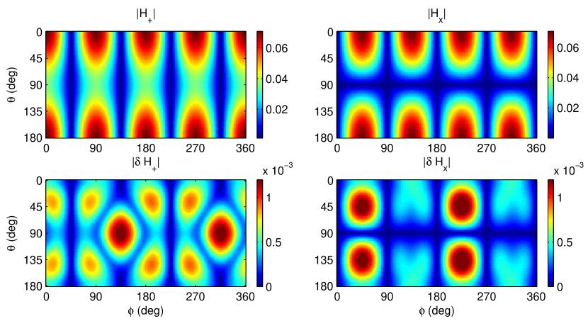
Figure 4: Top row: the normalized detector responses to $+$ and $\times$ polarisations, bottom row: the magnitude of the error. All these quantities are calculated at 1.2 kHz for comparison with [17].

4.3 Variations of the interferometer arm lengths

In the following analysis, we will also need to consider the response of the interferometer to changes of its arm lengths. Such a detector response is commonly used in calibration measurements. If $x_{1}$ and $x_{2}$ are the displacements of the front and back mirrors of one of the arm cavities, the change in the distance between the mirrors, as seen by the light propagating in the cavity, is

$$\delta L(t)=x_{2}(t-T)-x_{1}(t)\,,$$ (34)

where $T$ is the photon transit time ($T=L/c$). In this case, the signal is

$$\tilde{V}(f) = \mu\,C(f)\delta\tilde{L}(f)$$ (35)

$$= \mu\,C(f)\left[\rme^{-i2\pi fT}\tilde{x}_{2}(f)-\tilde{x}_{1}(f)\right],$$

where $C(f)$ is given by (27). (For derivation of (34) and (35), see [21].) At low frequencies, this response can be approximated by

$$\tilde{V}(f)\approx\mu\left[C_{\mathrm{pole}}(f)\,\tilde{x}_{2}(f)-C_{\mathrm{zp}}(f)\,\tilde{x}_{1}(f)\right].$$ (36)

The relative error between the exact (35) and approximate formula (36) is less than 1% for the front mirror and 0.5% for back mirror for frequencies up to 2 kHz.

5 Effect on searches for periodic gravitational waves

A gravitational-wave signal from a pulsar is quasi-periodic and therefore greatly benefits from synchronous detection (heterodyne method) [23]. This method removes the dominant oscillatory part of the signal at frequency $f$, and corrects for any phase modulation (Doppler shift) due to the rotation of the Earth and its orbital motion relative to the pulsar, as well as any possible pulsar frequency evolution (e.g., spin-down). If we ignore variations in the detector response due to these small frequency shifts, the output of the heterodyne method is given by the following (complex) signal

$$y(t)=\frac{1}{2}\left[H_{+}(\hat{n},f;t)\frac{1}{2}(1+\cos^{2}\iota)-iH_{\times}(\hat{n},f;t)\cos\iota\right]h_{0}e^{i\phi_{0}},$$ (37)

where $h_{0}$ is the amplitude, $\iota$ the inclination angle, and $\phi_{0}$ the initial phase of the heterodyne transformation. There is also an implicit dependence on the polarisation angle $\beta$ which enters the signal through the detector response functions. The remaining time dependence in (37) comes from the sidereal rotation of unit vectors $\hat{a}$ and $\hat{b}$ which are fixed to the Earth.

The use of the long-wavelength approximation affects both detection sensitivity and parameter estimation. For simplicity, assume that all parameters of the pulsar signal are known except for the amplitude $h_{0}$. Then the relevant quantities are

$$\epsilon=1-\frac{\langle y,z\rangle}{\sqrt{\langle y,y\rangle}\,\sqrt{\langle z,z\rangle}}\quad{\mathrm{and}}\quad\delta=\frac{\langle y,z\rangle}{\langle z,z\rangle}-1\,,$$ (38)

where $y(t)$ is given by (37) and $z(t)$ is calculated with the same expression except that $H_{A}$ are replaced with $H_{A}^{\mathrm{approx}}$ given in (33). The inner product is defined as

$$\langle y_{u},y_{v}\rangle=\int{\mathrm{Re}}\left[y_{u}(t)y_{v}^{*}(t)\right]\rmd t\,,$$ (39)

where the integration is taken over one sidereal day. It can be shown that $\epsilon$ is the fractional change in signal-to-noise ratio, and $\delta$ is the fractional bias in the estimate of the amplitude of the gravitational wave, both caused by the use of the inaccurate detector response [24].

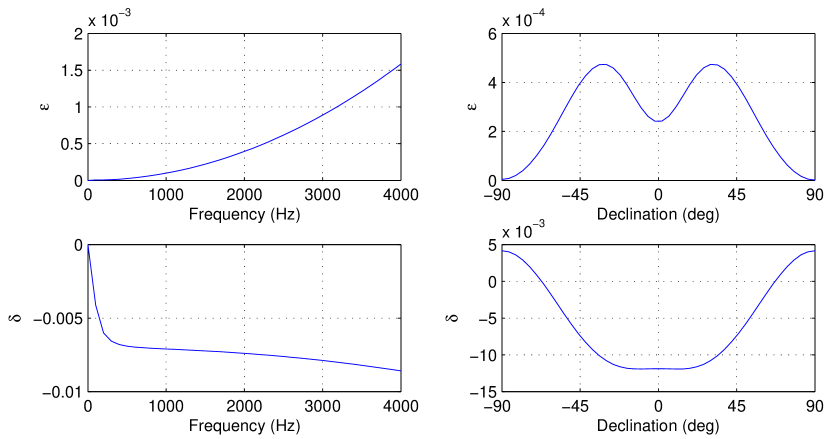
Figure 5: $\epsilon$ and $\delta$ as a function of frequency for ${\mathrm{dec}}=45^{\circ}$ (left), and as a function of declination for $f=2$ kHz (right). (Other parameters are $\beta=0$, $\iota=0$, and $\phi_{0}=0$.)

Figure 5 shows $\epsilon$ and $\delta$ as a function of the frequency of the gravitational wave for fixed source declination, and also as a function of the declination angle for fixed frequency, for the 4-km LIGO Hanford interferometer. For source location, we only need to specify the declination angle as the dependence on the right ascention is removed by the 24-hour sidereal-time integration. For simplicity, we assumed that $\beta=\iota=\phi_{0}=0$, which corresponds to a circularly-polarised gravitational wave. One can see from the figure that the change in the snr, $\epsilon$, is much less than 1% for all directions on the sky and all frequencies up to 4 kHz. Also, the bias, $\delta$, in the estimation of $h_{0}$ is less than 1.5% for all directions on the sky at $f=2$ kHz.

6 Effect on searches for stochastic gravitational waves

Consider an isotropic, unpolarised stochastic gravitational-wave background and assume that it is described by a stationary Gaussian random process. Then the expectation value of the cross-correlation [8, 25, 26] of the outputs of two detectors is proportional to the overlap reduction function:

$$\Gamma(f)=\frac{5}{8\pi}\int_{S^{2}}\rmd^{2}\Omega_{\hat{n}}H_{1A}(\hat{n},f)H^{*}_{2A}(\hat{n},f)e^{i2\pi f\hat{n}\cdot(\vec{x}_{1}-\vec{x}_{2})/{c}}\,,$$ (40)

where $\vec{x}_{1}$ and $\vec{x}_{2}$ are the locations of the two detectors on Earth and $H_{1A}(\hat{n},f)$ and $H_{2A}(\hat{n},f)$ are their response functions. (The summation over polarisation indices $A$ is understood.) Figure 6 shows a typical $\Gamma(f)$ calculated with both the exact (31) and approximate (33) formulae. The two detectors are the 4-km LIGO Hanford (H1) and Livingston (L1) interferometers.

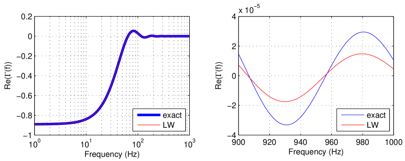
Figure 6: Overlap reduction function for LIGO H1 and L1 interferometers, calculated using the long-wavelength and exact detector response functions. Left: ${\rm Re}(\Gamma(f))$ for frequency range from 1 Hz to 1 kHz. Right: a small section of the plot magnified to show the slight difference between the two curves.

The error in the detector response from the long-wavelength approximation affects detection sensitivity and parameter estimation via the overlap reduction function. The two relevant quantities are

$$\epsilon=1-\frac{\langle\Gamma,\Gamma_{\ell.w.}\rangle}{\sqrt{\langle\Gamma,\Gamma\rangle}\sqrt{\langle\Gamma_{\ell.w.},\Gamma_{\ell.w.}\rangle}}\quad{\mathrm{and}}\quad\delta=\frac{\langle\Gamma,\Gamma_{\ell.w.}\rangle}{\langle\Gamma_{\ell.w.},\Gamma_{\ell.w.}\rangle}-1\,,$$ (41)

where $\Gamma(f)$ is given by (40) and $\Gamma_{\ell.w.}(f)$ is calculated with the same expression except that $H_{A}$ are replaced with $H_{A}^{\mathrm{approx}}$ given in (33). The inner product is defined as

$$\langle\Gamma_{u},\Gamma_{v}\rangle=\int_{f_{\rm min}}^{f_{\rm max}}\frac{{\rm Re}\left[\Gamma^{*}_{u}(f)\Gamma_{v}(f)\right]}{f^{6}Q_{1}(f)Q_{2}(f)}\rmd f\,,$$ (42)

where $Q_{1,2}(f)$ are the power spectra of the outputs of the two detectors. It can be shown that $\epsilon$ is the fractional change in signal-to-noise ratio, and $\delta$ is the fractional bias in the cross-correlation statistic, both caused by the use of the inaccurate detector response [24]. In this calculation, we also took into account the systematic error from the single-pole approximation to the cavity response [see (36)] which occurs when the detector output is calibrated.

Table 1 shows $\epsilon$ and $\delta$ corresponding to several detector cross correlations. The upper part of the table gives the values for the LIGO-ALLEGRO search for a stochastic background [28], which involved correlations of the Livingston interferometer with the ALLEGRO bar detector in a narrow band of frequencies near its peak sensitivity at 915 Hz. The search was performed with three different orientations of the bar detector: parallel to the X-arm of the interferometer (AX), parallel to the Y-arm (AY), and parallel to the bisector of the two arms (AN), also known as the null orientation. We find that the upper limits in [28] are not affected to the stated precision by the corrections in $\Gamma$.

Table 1: The fractional snr change, $\epsilon$, and the fractional bias, $\delta$, for an isotropic stochastic background. Here we assumed that the stochastic background has constant energy density in the frequency band of interest $[f_{\rm min},f_{\rm max}]$, and used the nominal design sensitivities of the instruments. (For details, see [24].)

• $f$		LIGO–ALLEGRO
  $915$ Hz		L1-AX	L1-AY	L1-AN
  	$\epsilon$	$\hbox{\phantom{-}}3.6$e-7	$\hbox{\phantom{-}}3.6$e-7	$\hbox{\phantom{-}}3.6$e-7
  	$\delta$	$-4.1$e-3	$-5.3$e-3	$-2.6$e-2
  $[f_{\mathrm{min}},f_{\mathrm{max}}]$		LIGO–VIRGO
  $50-150$ Hz		-H1-L1	-H1-V1	-L1-V1
  	$\epsilon$	$\hbox{\phantom{-}}4.0$e-6	$\hbox{\phantom{-}}1.5$e-6	$\hbox{\phantom{-}}1.5$e-6
  	$\delta$	$-6.6$e-3	$-5.5$e-3	$-5.5$e-3
  $900-1000$ Hz		-H1-L1	-H1-V1	-L1-V1
  	$\epsilon$	$\hbox{\phantom{-}}1.2$e-3	$\hbox{\phantom{-}}3.1$e-5	$\hbox{\phantom{-}}2.2$e-5
  	$\delta$	$\hbox{\phantom{-}}2.7$e-2	$-1.5$e-2	$-1.5$e-2

The rest of the table gives the values for $\epsilon$ and $\delta$ corresponding to various choices of cross-correlation between the LIGO and VIRGO (V1) interferometers. The first frequency band, 50-150 Hz, corresponds to the best sensitivity of the LIGO detectors. The second frequency band, 900-1000 Hz, is motivated by the VIRGO detector. At the present, this is where it contributes the most to the correlation-based searches. Note that only the H1-L1 low frequency analysis has been done so far, see e.g., [29]. The other interferometer cross-correlations will be performed in the future. One can see from the table that all these errors are less than 1%, except for the LIGO-VIRGO correlation searches around 1 kHz, which would have a 1-2% fractional bias in parameter estimation.

7 Summary

We re-evaluated high-frequency corrections to the detector response and analysed their effect on current searches for gravitational waves with km-scale laser interferometers. Using the exact formula for the detector response, we estimated systematic errors introduced by the long-wavelength approximation in detection sensitivity and parameter estimation of gravitational waves. Typical examples were taken from searches for periodic gravitational waves and from searches for an isotropic stochastic background. So far, in all cases considered, the errors are at most 1-2% and somewhat smaller than the previously reported 10% error at 1.2 kHz [17].

We have thus shown that the long-wavelength approximation for Michelson-Fabry-Perot interferometer (33) was sufficiently accurate for searches performed to date, which were limited to frequencies below 2 kHz. However, extending the analysis to higher frequencies will likely require using the exact formula for the detector response (31). For example, the exact formula is essential in searches for burst [30] and stochastic gravitational waves [31] at the free-spectral-range frequency (37.5 kHz) of LIGO interferometers. Future searches for stochastic gravitational waves can go to even higher frequencies [32]. In conclusion, we recommend the use of the exact formula whenever the accuracy of the detector response is important.

References

References

- [1] Barish B and Weiss R 1999 Phys. Today 52 44
- [2] Bradaschia C et al. 1990 Nucl. Instrum. Methods 289 518
- [3] Misner C, Thorne K and Wheeler J 1973 Gravitation (San Francisco: W.H. Freeman and Company)
- [4] Thorne K 1987 in S Hawking and W Israel, eds, 300 Years of Gravitation (Chicago: University of Chicago Press)
- [5] Gürsel Y, Linsay P, Spero R, Saulson P, Whitcomb S and Weiss R 1984 in A Study of a Long Baseline Gravitational Wave Antenna System (National Science Foundation Report)
- [6] Meers B 1989 Phys. Lett.A 142 465
- [7] Christensen N 1990 On Measuring the Stochastic Gravitational Radiation Background with Laser Interferometric Antennas Ph.D. thesis Massachusetts Institute of Technology
- [8] Christensen N 1992 Phys. Rev.D 46 5250
- [9] Sigg D 1997 Strain calibration in LIGO. LIGO Technical Report T970101
- [10] Mizuno J, Rüdiger A, Schilling R, Winkler W and Danzmann K 1997 Opt. Comm. 138 383
- [11] Rakhmanov M 2005 Phys. Rev.D 71 084003
- [12] Estabrook F and Wahlquist H 1975 Gen. Relativ. Gravit. 6 439
- [13] Estabrook F 1985 Gen. Relativ. Gravit. 17 719
- [14] Schilling R 1997 Class. Quantum Grav. 14 1513
- [15] Larson S, Hiscock W and Hellings R 2000 Phys. Rev.D 62 062001
- [16] Cornish N and Rubbo L 2003 Phys. Rev.D 67 022001
- [17] Baskaran D and Grishchuk L 2004 Class. Quantum Grav. 21 4041
- [18] Schutz B and Tinto M 1987 Mon. Not. R. Astr. Soc. 224 131
- [19] Rakhmanov M 2006 Response of LIGO 4-km interferometers to gravitational waves at high frequencies and in the vicinity of the FSR (37.5 kHz). LIGO Technical Report T060237
- [20] Whelan J 2007 Higher-frequency corrections to stochastic formulae. LIGO Technical Report T070172
- [21] Rakhmanov M, Savage R, Reitze D and Tanner D 2002 Phys. Lett.A 305 239
- [22] Hunter E 2005 Analysis of the frequency dependence of the LIGO directional sensitivity (antenna pattern) and implications for detector calibration. LIGO Technical Report T050136
- [23] Dupuis R and Woan G 2005 Phys. Rev.D 72 102002
- [24] Woan G and Romano J D 2008 Effects of using the wrong antenna pattern on sensitivity and parameter estimation. LIGO Technical Report T080134
- [25] Flanagan É 1993 Phys. Rev.D 48 2389
- [26] Cornish N and Larson S 2001 Class. Quantum Grav. 18 3473
- [27] Allen B and Romano J 1999 Phys. Rev.D 59 102001
- [28] Abbott B et al. 2007 Phys. Rev.D 76 022001
- [29] Abbott B et al. 2007 Astrophys. J. 659 918
- [30] Parker J 2007 Development of a high-frequency burst analysis pipeline. LIGO Technical Report T070037
- [31] Forrest C, Fricke T, Giampanis S and Melissinos A 2007 Search for a diurnal variation of the power detected at the FSR frequency. LIGO Technical Report T070228
- [32] Nishizawa A et al. 2008 Phys. Rev.D 77 022002