Numerical diagonalization analysis of the criticality of the $(2+1)$-dimensional $XY$ model: Off-diagonal Novotny’s method

Abstract

The criticality of the $(2+1)$-dimensional $XY$ model is investigated with the numerical diagonalization method. So far, it has been considered that the diagonalization method would not be very suitable for analyzing the criticality in large dimensions ($d\geq 3$); in fact, the tractable system size with the diagonalization method is severely restricted. In this paper, we employ Novotny’s method, which enables us to treat a variety of system sizes $N=6,8,\dots,20$ ($N$: the number of spins constituting a cluster). For that purpose, we develop an off-diagonal version of Novotny’s method to adopt the off-diagonal (quantum-mechanical $XY$) interaction. Moreover, in order to improve the finite-size-scaling behavior, we tune the coupling-constant parameters to a scale-invariant point. As a result, we estimate the critical indices as $\nu=0.675(20)$ and $\gamma/\nu=1.97(10)$.

I Introduction

It has been considered that the diagonalization method would not be very suitable for analyzing the criticality in large dimensions $d\geq 3$. In fact, as the system size enlarges, the number of spins constituting a cluster increases rapidly in $d\geq 3$, and the dimensionality of the Hilbert space soon exceeds the limitation of available computer resources. Such a severe limitation as to the tractable system size prevents us from making a systematic analysis of the simulation data.

To cope with this difficulty, Novotny proposed a transfer-matrix formalism Novotny90 ; Novotny92 ; Novotny91 , which enables us to construct a transfer-matrix unit with an arbitrary (integral) number of spins $N$; note that conventionally, the number of spins is restricted within $N=2^{d-1},3^{d-1},\dots$. As a demonstration, Novotny simulated the Ising model in $d\leq 7$ systematically Novotny91 . Meanwhile, it has been shown that the idea is applicable to a wide class of systems such as the frustrated Ising model Nishiyama04 and the quantum-mechanical Ising model under the transverse magnetic field Nishiyama07 .

In this paper, we extend the Novotny method to adopt the off-diagonal (quantum-mechanical $XY$) interaction; see the Hamiltonian, Eq. (1), mentioned afterward. Actually, as mentioned above, the use of Novotny’s method has been restricted within the case of the diagonal (Ising-type) interaction. As a demonstration, we apply the method to the $(2+1)$-dimensional $XY$ model with a variety of system sizes $N=6,8,\dots,20$. Taking the advantage that a series of system sizes are available, we made a systematic finite-size-scaling analysis of the simulation data. As a result, we estimate the critical indices as $\nu=0.675(20)$ and $\gamma/\nu=1.97(10)$. Recent developments on the $d=3$ $XY$ universality class are overviewed in Ref. Barmatz07 with an emphasis on the microgravity-environment experiment; see also Refs. Buteral97 ; Guida98 ; Kleinert05 ; Burovski06 ; Campostrini06 . Our method provides an alternative approach to the $d=3$ $XY$ universality class.

To be specific, we consider the following Hamiltonian for the $(2+1)$-dimensional $XY$ model Costa03 ; Leonel06 ; Dely06 with the extended interactions

$${\cal H}=-J_{NN}\sum_{\langle ij\rangle}(S^{x}_{i}S^{x}_{j}+S^{y}_{i}S^{y}_{j})-J_{NNN}\sum_{\langle\langle ij\rangle\rangle}(S^{x}_{i}S^{x}_{j}+S^{y}_{i}S^{y}_{j})+D_{\Box}\sum_{[ijkl]}(S^{z}_{i}+S^{z}_{j}+S^{z}_{k}+S^{z}_{l})^{2}+D\sum_{i}(S^{z}_{i})^{2}.$$ (1)

Here, the quantum spin-1 ($S=1$) operators $\{{\bf S}_{i}\}$ are placed at each square-lattice point $i$. The summations, $\sum_{\langle ij\rangle}$, $\sum_{\langle\langle ij\rangle\rangle}$, and $\sum_{[ijkl]}$, run over all possible nearest-neighbor, next-nearest-neighbor, and plaquette spins, respectively. The parameters, $J_{NN}$, $J_{NNN}$, and $D_{\Box}$, are the corresponding coupling constants. The single-ion anisotropy $D$, drives the system from the $XY$ phase ($D<D_{c}$) to the large-$D$ phase ($D>D_{c}$). (In the large-$D$ phase, the ground state is magnetically disordered, accompanied with a finite excitation gap.) Our aim is to survey the criticality by means of the off-diagonal Novotny method.

The Hamiltonian (1) has a number of tunable parameters. We fixed them to

$$(J_{NN},J_{NNN},D_{\Box})=(0.158242810160,0.058561393564,0.10035104389),$$ (2)

and survey the $D$-driven phase transition. As explicated in the Appendix, around the point (2), the finite-size-scaling behavior improves significantly; the irrelevant interactions cancel out, because the point (2) is a scale-invariant point with respect to the real-space decimation shown in Fig. 9. Such an elimination of finite-size corrections has been utilized successfully to analyze the criticality of the classical systems such as the Ising model Blote96 ; Nishiyama06 and the lattice $\phi^{4}$ theory Ballesteros98 ; Hasenbusch99 . We adopt the idea to investigate a quantum-mechanical system, Eq. (1).

The rest of this paper is organized as follows. In Sec. II, we develop an off-diagonal version of the Novotny method. In Sec. III, employing this method, we simulate the $(2+1)$-dimensional $XY$ model (1). In Sec. IV, we present the summary and discussions. In the Appendix, we determine a scale-invariant point (2) with respect to the real-space decimation shown in Fig. 9.

II Off-diagonal Novotny’s method

In this section, we explain the simulation scheme. As mentioned in the Introduction, we develop an off-diagonal version of Novotny’s method to simulate the $(2+1)$-dimensional $XY$ model (1); so far, the Novotny method has been applied to the case of Ising-type interactions Novotny90 ; Novotny92 ; Novotny91 ; Nishiyama04 ; Nishiyama07 .

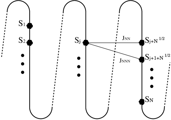
Figure 1: A schematic drawing of the spin cluster for the $d=2$ quantum $XY$ model (1) is presented. As indicated above, the spins constitute a one-dimensional alignment $\{S_{i}\}$ ($i=1,2,\dots,N$), and the dimensionality is lifted to $d=2$ by the bridges over the $(N^{1/2})$th-neighbor pairs. This is a basic idea of Novotny’s diagonalization method. We need to develop an off-diagonal version of Novotny’s method, because we have to adopt the quantum $XY$ interaction (1); see Sec. II.

To begin with, we explain the basic idea of Novotny’s method. Novotny’s method allows us to construct a cluster with an arbitrary number of spins; see Fig. 1. As indicated, the basic structure of the cluster is one-dimensional. The dimensionality is lifted to $d=2$ by the bridges over the $(\sqrt{N})$-th-neighbor pairs. Because the basic structure is one-dimensional, we are able to construct a cluster with an arbitrary (integral) number of spins $\{{\bf S}_{i}\}$ ($i=1,2,\dots,N$); note that naively, the number of spins is restricted within $N=4,9,16,\dots$ in $d=2$.

We formulate the above idea explicitly. We propose the following expression

$${\cal H}=-J_{NN}(H_{XY}(1)+H_{XY}(\sqrt{N}))-J_{NNN}(H_{XY}(\sqrt{N}+1)+H(\sqrt{N}-1))+D_{\Box}H_{\Box}(\sqrt{N})+D\sum_{i=1}^{N}(S_{i}^{z})^{2},$$ (3)

for the Hamiltonian of the $(2+1)$-dimensional $XY$ model (1). The component $H_{XY(\Box)}(v)$ describes the $XY$ (plaquette) interaction over the $v$-th neighbor pairs; see Fig. 1. Because the quantum $XY$ interaction, $H_{XY}(v)$, is an off-diagonal one, we need to develop an off-diagonal version of Novotny’s method. We propose the following expression

$$H_{XY}(v)=\sum_{i=1}^{N}(P^{v}S^{x}_{i}P^{-v}S^{x}_{i}+P^{v}S^{y}_{i}P^{-v}S^{y}_{i}).$$ (4)

This formula serves as a basis of the off-diagonal Novotny method. The symbol $P$ denotes the translation operator by one lattice spacing;

$$P|S_{1},S_{2},\dots,S_{N}\rangle=|S_{N},S_{1},\dots,S_{N-1}\rangle.$$ (5)

(We impose the periodic boundary condition, $S_{N+1}=S_{1}$.) Here, the base $|\{S_{k}\}\rangle$ diagonalizes the $\{S^{z}_{i}\}$ operators; namely, it satisfies

$$S^{z}_{l}|\{S_{k}\}\rangle=S_{l}|\{S_{k}\}\rangle,$$ (6)

for each $l=1,2,\dots,N$. The insertions of the operators $P^{\pm v}$ in Eq. (4) introduce the $v$-th neighbor interaction along the alignment of spins $\{S_{i}\}$; symbolically, the operator $P^{v}S^{\alpha}_{i}P^{-v}$ may be written as $S^{\alpha}_{i+v}$. On the other hand, as for $H_{\Box}(v)$, we adopt the conventional idea based on the diagonal Novotny method Novotny90 . That is, its diagonal elements $\{\langle\{S_{k}\}|H_{\Box}(v)|\{S_{k}\}\rangle\}$ are given by

$$\langle\{S_{k}\}|H_{\Box}(v)|\{S_{k}\}\rangle=\langle\{S_{k}\}|P^{v}T|\{S_{k}\}\rangle,$$ (7)

with the four-spin interaction

$$\langle\{S_{k}\}|T|\{T_{k}\}\rangle=\sum_{l=1}^{N}S_{l}S_{l+1}T_{l}T_{l+1}.$$ (8)

Similarly, the insertion of $P^{v}$ introduces the $v$-th neighbor interaction. However, in the diagonal scheme (7), one operation of $P^{v}$ suffices; note that in the off-diagonal formalism (4), two operations $P^{\pm v}$ are required. Because each operation $P^{\pm v}$ requires huge computational effort, the off-diagonal scheme is computationally demanding. Afterward, we provide a number of formulae useful for the practical implementation of the algorithm.

The above formulae complete the formal basis of our simulation scheme. Aiming to improve the simulation result, we implement the following symmetrization technique Novotny92 . That is, we symmetrize the component $H_{XY,\Box}(v)$ by replacing it with

$$H_{XY,\Box}(v)\to(H_{XY,\Box}(v)+H_{XY,\Box}(-v))/2.$$ (9)

This replacement restores the symmetry between the ascending, $S_{1},S_{2},\dots,S_{N}$, and the descending, $S_{N},S_{N-1},\dots,S_{1}$, directions completely.

Last, we provide a number of formulae that may be useful in the practical implementation of the algorithm. We utilize the translationally invariant bases $\{|k,n\rangle\}$, which diagonalize the operator $P$;

$$P|k,n\rangle=e^{ik}|k,n\rangle.$$ (10)

Here, the wave number $k$ runs over a Brillouin zone $k=2\pi M/N$ ($M$: integer), and the index $n$ specifies the state within the subspace $k$. As anticipated, the bases $\{|k,n\rangle\}$ are useful to obtain an explicit representation of the formulae mentioned above. For instance, the first term of the formula (4) is represented by

$$\langle k,n|\sum_{j=1}^{N}S^{x}_{j}P^{v}S^{x}_{j}P^{-v}|k,m\rangle=\sum_{j=1}^{N}\sum_{k^{\prime},n^{\prime}}\langle k,n|S^{x}_{j}|k^{\prime},n^{\prime}\rangle\langle k^{\prime},n^{\prime}|S^{x}_{j}|k,m\rangle e^{i(k^{\prime}-k)v},$$ (11)

in terms of the frame $\{|k,n\rangle\}$. Because the parameter $v$ is, in general, an irrational number, the oscillating factor $e^{i(k^{\prime}-k)v}$ is incommensurate with respect to the lattice periodicity. Hence, the intermediate summation $\sum_{k^{\prime}}$ has to be treated carefully; namely, each Brillouin zone $\{k^{\prime}\}$ is no longer equivalent. We accepted the following symmetrized sum

$$\sum_{k^{\prime}}a_{k^{\prime}}=\frac{1}{2}a_{-\pi}+a_{-\pi+2\pi/N}+a_{-\pi+4\pi/N}+\dots+a_{\pi-2\pi/N}+\frac{1}{2}a_{\pi},$$ (12)

with respect to a summand $a_{k^{\prime}}$. Here, the denominators of the first and the last terms compensate the duplicated sum at the edges of the Brillouin zone $[-\pi,\pi]$. (Similarly, we obtain an explicit representation for $H_{\Box}(v)$ via the conventional Novotny method Novotny90 ; Novotny92 .) Provided that the explicit matrix elements of $H_{XY,\Box}(v)$ are at hand, we are able to perform the numerical diagonalization of the Hamiltonian (3). The results are shown in the next section.

Last, we make an overview of the $S=1$ $XY$ model (1). As mentioned in the Introduction, the model has been studied in Refs. Costa03 ; Leonel06 ; Dely06 . In the case of $d=1$ dimension, the criticality ($D$-driven phase transition) was investigated in detail Botet83 . According to Ref. Botet83 , for sufficiently large $D$, a magnetically disordered ground state (large-$D$ phase) appears, and the criticality is identical to that of the classical counterpart in $d+1(=2)$ dimensions (KT transition). Unfortunately, a naive extension to the case of $S=1/2$ is not appropriate, because the $D$ anisotropy, $D(S^{z}_{i})^{2}$, reduces to a constant term, $D/4$. (Moreover, the transverse magnetic field violates the $XY$ symmetry, and the criticality changes into the Ising type.) As a matter of fact, it is difficult to realize a ground-state phase transition for the $S=1/2$ model without violating the translational invariance and the rotational symmetry. (Possibly, the double-plane $S=1/2$ model may exhibit a desirable criticality by tuning the inter-plane interaction. However, this model is too complicated.) Hence, we consider the $S=1$ $XY$ model (1) with the $D$-anisotropy term.

III Numerical results

In this section, we analyze the criticality of the $(2+1)$-dimensional $XY$ model, Eq. (1). As mentioned in the Introduction, the coupling-constant parameters $(J_{NN},J_{NNN},D_{\Box})$ are set to the scale-invariant point (2). Thereby, we survey the $D$-driven phase transition with the finite-size scaling. In order to diagonalize the Hamiltonian, we utilize the off-diagonal Novotny method developed in Sec. II. Owing to this method, we treat a variety of system sizes $N=6,8,\dots,20$. The linear dimension $L$ of the cluster is given by

$$L=\sqrt{N},$$ (13)

because the $N$ spins constitute a rectangular cluster; see Fig. 1.

III.1 Transition point

In this section, we provide an evidence of the $D$-driven phase transition, and estimate the critical point $D_{c}$ with the finite-size scaling.

In Fig. 2, we plot the scaled energy gap $L\Delta E$ for various $D$, and $N=6,8,\dots,20$ with the other coupling constants fixed to Eq. (2). The symbol $\Delta E$ denotes the first-excitation gap. According to the finite-size scaling, the scaled energy gap $L\Delta E$ should be invariant at the critical point. Indeed, we observe an onset of the $D$-driven phase transition around $D\approx 1$.

In Fig. 3, we plot the approximate transition point $D_{c}(L_{1},L_{2})$ for $(2/(L_{1}+L_{2}))^{3}$ with $6\leq N_{1}<N_{2}\leq 20$ and $L_{1,2}=\sqrt{N_{1,2}}$; the validity of the $1/L^{3}$-extrapolation scheme (abscissa scale) is considered at the end of this section. Here, the approximate transition point $D_{c}(L_{1},L_{2})$ denotes a scale-invariant point with respect to a pair of system sizes $(L_{1},L_{2})$. Namely, the approximate transition point satisfies the equation

$$L_{1}\Delta E(L_{1})|_{D=D_{c}(L_{1},L_{2})}=L_{2}\Delta E(L_{2})|_{D=D_{c}(L_{1},L_{2})}.$$ (14)

The least-squares fit to the data of Fig. 3 yields $D_{c}=0.9569(83)$ in the thermodynamic limit, $L\to\infty$. As a reference, we calculated $D_{c}=0.9744(68)$ through the $1/L^{4}$-extrapolation scheme. Considering the deviation as an error indicator, we estimate the critical point as

$$D_{c}=0.957(25).$$ (15)

Let us mention a few remarks. First, we consider the abscissa scale $1/L^{3}$ utilized in Fig. 3. Naively, the scaling theory predicts that dominant corrections to $D_{c}$ should scale like $1/L^{\omega+1/\nu}$ with $\omega=0.785(20)$ and $\nu=0.6717(1)$ Campostrini06 . On one hand, in our simulation, such dominant corrections should be suppressed by tuning the coupling constants to Eq. (2); see the Appendix. The convergence to the thermodynamic limit may be accelerated Nishiyama06 . (For extremely large system sizes, the singularity $1/L^{\omega+1/\nu}$ may emerge.) Hence, in Fig. 3, we set the abscissa scale to $1/L^{3}$. Second, we argue a consistency between the finite-size scaling and the real-space decimation; in the Appendix, we made a fixed-point analysis (34), regarding $D$ as a unit of energy $D=1$ (30). This proposition $D=1$ is quite consistent with the above scaling result (15), validating the fixed-point analysis in the Appendix. In other words, around the fixed point (34), corrections to scaling may cancel out satisfactorily. Encouraged by this consistency, in Sec. III.3, we survey the criticality rather in detail.

III.2 Comparison with the conventional $XY$ model

In the preceding section, we simulated the $XY$ model (1) with the finely tuned coupling constants (2). As a comparison, in this section, we provide the data for the conventional $XY$ model. That is, we turn off the extended coupling constants, setting the interactions to $(J_{NN},J_{NNN},D_{\Box})=(0.2,0,0)$ tentatively.

In Fig. 4, we plot the scaled energy gap $L\Delta E$ for various $D$ and $N=6,8,\dots,20$. We observe an onset of the $D$-driven phase transition around $D\approx 1.1$. However, the data are scattered, as compared to those of Fig. 2. In fact, in Fig. 4, the location of the transition point appears to be less clear. This result demonstrates that the finely-tuned coupling constants (2) lead to elimination of finite-size corrections.

III.3 Critical exponents

In Sec. III.1, we observe an onset of the $D$-driven phase transition. In this section, we calculate the critical exponents, $\nu$ and $\gamma/\nu$, based on the finite-size scaling.

In Fig. 5, we plot the approximate critical exponent

$$\nu(L_{1},L_{2})=\frac{\ln(L_{1}/L_{2})}{\ln(\partial_{D}(L_{1}\Delta E(L_{1}))/\partial_{D}(L_{2}\Delta E(L_{2})))|_{D=D_{c}}},$$ (16)

for $(2/(L_{1}+L_{2}))^{2}$ with $6\leq N_{1}<N_{2}\leq 20$ ($L_{1,2}=\sqrt{N_{1,2}}$), and $D_{c}=0.957$ [Eq. (15)]; afterward, we consider the abscissa scale, $1/L^{2}$. The least-squares fit to these data yields $\nu=0.675(16)$. As a reference, we calculated $\nu=0.687(11)$ through the $1/L^{3}$-extrapolation scheme. Considering the deviation as an error indicator, we estimate the critical exponent as

$$\nu=0.675(20).$$ (17)

In Fig. 6, we plot the approximate critical exponent

$$\gamma/\nu=\ln(\chi_{\perp}(L_{1})/\chi_{\perp}(L_{2}))|_{D=D_{c}}/\ln(L_{1}/L_{2}),$$ (18)

for $(2/(L_{1}+L_{2}))^{2}$ with $6\leq N_{1}<N_{2}\leq 20$ ($L_{1,2}=\sqrt{N_{1,2}}$), and $D_{c}=0.957$ [Eq. (15)]. Here, the transverse susceptibility $\chi_{\perp}$ is given by the resolvent form

$$\chi_{\perp}=\frac{1}{N}\langle g|M_{x}\frac{1}{{\cal H}-E_{g}}M_{x}|g\rangle,$$ (19)

with the ground state $|g\rangle$ and the ground-state energy $E_{g}$. The magnetization $M_{x}$ is given by $M_{x}=\sum_{i=1}^{N}S_{i}^{x}$. The resolvent form (19) is readily calculated with use of the continued-fraction method Gagliano87 .

The least-squares fit to the data in Fig. 6 yields $\gamma/\nu=1.965(61)$. As a reference, we calculated $\gamma/\nu=2.020(42)$ through the $1/L^{3}$-extrapolation scheme. Considering the deviation as an error indicator, we estimate the critical exponent as

$$\gamma/\nu=1.97(10).$$ (20)

Last, we argue the abscissa scale $1/L^{2}$ utilized in Figs. 5 and 6. Naively, the scaling theory predicts that dominant corrections to the critical indices should scale like $1/L^{\omega}$ with $\omega=0.785(20)$ Campostrini06 . On one hand, as argued in Sec. III.1, such dominant corrections should be suppressed by adjusting the coupling constants to Eq. (2), and the convergence is accelerated than the naively expected one Nishiyama06 . Hence, we set the abscissa scale to $1/L^{2}$ in Figs. 5 and 6.

III.4 Refined data analysis

In this section, we make an alternative analysis of the criticality to demonstrate a reliability of our scheme.

In Figs. 7 and 8, we plot the critical exponents

$$\nu=\frac{\ln(L_{1}/L_{2})}{\ln(\partial_{D}(L_{1}\Delta E(L_{1}))/\partial_{D}(L_{2}\Delta E(L_{2})))|_{D=D_{c}(L_{1},L_{2})}},$$ (21)

and

$$\gamma/\nu=\ln(\chi_{\perp}(L_{1})/\chi_{\perp}(L_{2}))|_{D=D_{c}(L_{1},L_{2})}/\ln(L_{1}/L_{2}),$$ (22)

respectively, for $(2/(L_{1}+L_{2}))^{2}$ with $6\leq N_{1}<N_{2}\leq 20$. Here, these exponents are calculated at the approximate critical point $D=D_{c}(L_{1},L_{2})$ (14) rather than at $D_{c}=0.957$ as in the preceding section.

Clearly, these data, Figs. 7 and 8, exhibit accelerated convergence to the thermodynamic limit as compared to those of Figs. 5 and 6. In fact, the least-squares fit to these data yields the estimates $\nu=0.658(5)$ and $\gamma/\nu=1.946(4)$ with suppressed error margins. Actually, in Fig. 8, the systematic error dominates the insystematic one. In such a case, one has to make a detailed consideration of the nature of corrections to scaling to ensure the accuracy (amount of error margin) of the extrapolation. Here, we do not commence making such a consideration, and accept the estimates, Eqs. (17) and (20), obtained less ambiguously in the preceding section. It is not the purpose of this paper to obtain fully refined estimates for the critical indices. Such a detailed analysis will be pursued in the succeeding works. In fact, the diagonalization method has a potential applicability to the frustrated magnetism, for which the quantum Monte Carlo method suffers from the notorious sign problem. The Novotny method would be particularly of use to explore such a problem. Actually, in the case of the Ising-type anisotropy, the Novotny method was applied Nishiyama07b to clarifying the nature of the frustration-driven transition (Lifshitz point). The present scheme may provide a basis for surveying such a quantum frustrated system with the $XY$-type symmetry.

IV Summary and discussions

The criticality of the $(2+1)$-dimensional $XY$ model (1) was investigated with the numerical-diagonalization method. For that purpose, we developed an off-diagonal version of Novotny’s diagonalization method (Sec. II), which enables us to treat a variety of system sizes $N=6,8,\dots,20$ ($N$: the number of spins within a cluster). Moreover, we improved the finite-size-scaling behavior by adjusting the coupling-constant parameters to a scale-invariant point (2).

Owing to these improvements, we could analyze the simulation data systematically with the finite-size scaling. As a result, we estimated the critical indices as $\nu=0.675(20)$ and $\gamma/\nu=1.97(10)$. These indices immediately yield the following critical exponents

$$\alpha=-0.025(60),\beta=0.348(49),\ and\ \gamma=1.330(78),$$ (23)

through the scaling relations.

Recent developments on the $d=3$ $XY$ universality class are overviewed in Ref. Barmatz07 . Our diagonalization result (23) is accordant with a Monte Carlo result, $\alpha=-0.0151(3)$, $\beta=0.3486(1)$, and $\gamma=1.3178(2)$ Campostrini06 , and a field-theoretical result, $\alpha=-0.011(4)$, $\beta=0.3470(16)$, and $\gamma=1.3169(20)$ Guida98 . (In Ref. Campostrini06 , information from a series-expansion result is also taken into account.) To the best of our knowledge, no numerical-diagonalization result has been reported as for the $d=3$ $XY$ universality class. According to Ref. Barmatz07 , there arose a discrepancy between the Monte Carlo simulation and the microgravity-environment experiment; see also Ref. Pogorelov07 . As a matter of fact, the microgravity experiment Lipa03 reports a critical exponent $\alpha=-0.0127(3)$. In order to resolve this discrepancy, an alternative scheme other than the Monte Carlo and series-expansion methods would be desirable. Refinement of the diagonalization scheme through considering the singularity of corrections to scaling might be significant in order to settle this longstanding issue.

Appendix A Search for a scale-invariant point: Elimination of finite-size corrections

As mentioned in the Introduction, we simulated the quantum $XY$ model (1), setting the coupling constants to Eq. (2); around this point, we observe eliminated finite-size corrections. In this Appendix, we explicate the scheme to determine the point (2).

To begin with, we explain the technique to suppress the finite-size corrections. According to Refs. Blote96 ; Nishiyama06 ; Ballesteros98 ; Hasenbusch99 , the finite-size behavior improves around the renormalization-group fixed point. That is, the irrelevant interactions may cancel out around the fixed point. Clearly, such an improvement of the finite-size behavior admits us to make a systematic finite-size-scaling analysis of the simulation data. To avoid confusion, we stress that the fixed-point analysis is simply a preliminary one, and subsequently, we perform large-scale computer simulation to estimate the critical exponents. In this sense, as for the Monte Carlo simulation, it might be more rewarding to enlarge the system size rather than to extend the coupling-constant parameters and adjust them. On one hand, it is significant for the numerical diagonalization to eliminate corrections to scaling, because its tractable system size is restricted intrinsically.

In Fig. 9, we present a schematic drawing of the real-space-decimation procedure. As indicated, we consider a couple of rectangular clusters with the sizes $2\times 2$ and $4\times 4$. These clusters are labeled by the symbols $S$ and $L$, respectively. Decimating out the spin variables indicated by the symbol $\bullet$ within the $L$ cluster, we obtain a coarse-grained lattice identical to the $S$ cluster. Our aim is to search for a scale-invariant point with respect to the real-space decimation.

Before going into the fixed-point analysis, we set up the simulation scheme for the clusters, $S$ and $L$. We cast the Hamiltonian (1) into the following plaquette-based expression

$${\cal H}=\sum_{[ijkl]}{\cal H}^{\Box}_{ijkl}+D\sum_{i}(S^{z}_{i})^{2},$$ (24)

with the plaquette interaction

$${\cal H}^{\Box}_{ijkl} = -\frac{J_{NN}}{2}(S^{x}_{i}S^{x}_{j}+S^{y}_{i}S^{y}_{j}+S^{x}_{j}S^{x}_{l}+S^{y}_{j}S^{y}_{l}+S^{x}_{k}S^{x}_{l}+S^{y}_{k}S^{y}_{l}+S^{x}_{i}S^{x}_{k}+S^{y}_{i}S^{y}_{k})$$ (27)

$$-J_{NNN}(S^{x}_{i}S^{x}_{l}+S^{y}_{i}S^{y}_{l}+S^{x}_{j}S^{x}_{k}+S^{y}_{j}S^{y}_{k})$$

$$+D_{\Box}(S^{z}_{i}+S^{z}_{j}+S^{z}_{k}+S^{z}_{l})^{2}.$$

(The denominator of the coefficient $J_{NN}$ compensates the duplicated sum.) Hence, the Hamiltonian for the $S$ cluster is given by

$${\cal H}_{S}={\cal H}^{\Box}_{1234}+D\sum_{i=1}^{4}(S^{z}_{i})^{2},$$ (28)

with the replacement

$$J_{NN,NNN}\to(1+b)J_{NN,NNN}.$$ (29)

Here, the parameter $b$ controls the boundary interaction strength, and hereafter, we set $b=0.7$; we consider the validity of this choice afterward. The boundary-interaction parameter $b$ interpolates smoothly the open, $b=0$, and periodic, $b=1$, boundary conditions. The point is that for the two-site ($L=2$) system, the bulk interaction, $S^{\alpha}_{1}S^{\alpha}_{2}$, and the boundary interaction $S^{\alpha}_{2}S^{\alpha}_{1}$ coincide each other. Hence, for the $S$ cluster, the boundary interaction $b$ is freely tunable without violating the translation invariance. We make use of this redundancy to obtain the fixed point reliably. On the other hand, the $L$ cluster does not have such a redundancy, and the Hamiltonian ${\cal H}_{L}$ is given by Eq. (1) with $L=4$ unambiguously. We diagonalize these Hamiltonian matrices ${\cal H}_{S,L}$ numerically; note that we employ the conventional diagonalization method, rather than the off-diagonal Novotny method developed in Sec. II.

With use of the simulation technique developed above, we search for the fixed point of the real-space decimation. We survey the parameter space $(J_{NN},J_{NNN},D_{\Box})$, regarding $D$ as a unit of energy; namely, we set

$$D=1,$$ (30)

throughout this section. Thereby, we impose the following conditions

$$2\Delta E_{S} = 4\Delta E_{L}$$ (31)

$$\langle S^{x}_{1}S^{x}_{2}\rangle_{S} = \langle\tilde{S}^{x}_{1}\tilde{S}^{x}_{2}\rangle_{L}$$ (32)

$$\langle S^{x}_{1}S^{x}_{4}\rangle_{S} = \langle\tilde{S}^{x}_{1}\tilde{S}^{x}_{4}\rangle_{L},$$ (33)

as a scale-invariance criterion. The symbol $\Delta E_{S,L}$ denotes the excitation gap for the respective clusters. The arrangement of the spin variables, $S_{1,2,3,4}^{\alpha}$ and $\tilde{S}_{1,2,3,4}^{\alpha}$, is shown in Fig. 9. The symbol $\langle\dots\rangle_{S,L}$ denotes the ground-state average for the respective clusters. The first equality (31) comes from the scale invariance of the scaled energy gap, $L\Delta E$. (We refer readers to Ref. Itakura03 , where the author utilizes such a critical-amplitude relation successfully to analyze the renormalization-group flow numerically.) On one hand, the remaining equations, (32) and (33), are the scale-invariance conditions Swendsen82 regarding the correlation functions for the edge and diagonal spins, respectively.

The conditions, Eqs. (31)-(33), are the nonlinear equations with respect to $(J_{NN},J_{NNN},D_{\Box})$. In order to obtain the solution, we employed the Newton method, and found that the following nontrivial solution does exist;

$$(J_{NN},J_{NNN},D_{\Box})=(0.158242810160,0.058561393564,0.10035104389).$$ (34)

The last digits may be uncertain because of the round-off errors.

Last, we argue the validity of the above solution (34) and the boundary condition $b=0.7$. In Sec. III, via the finite-size-scaling analysis, we obtained $D_{c}=0.957(25)$ (15). Apparently, this result is consistent with $D=1$ postulated in Eq. (30). Moreover, the simulation data in Fig. 2 exhibit suppressed finite-size corrections, as compared to those of the ordinary $XY$ model, Fig. 6. These features validate the choice of the boundary condition $b=0.7$ as well as the reliability of the fixed point (34). Furthermore, we point out that the boundary condition $b=0.7$ is reminiscent of $b=0.4$ utilized in the fixed-point analysis of the $d=3$ Ising ferromagnet Nishiyama06 .

Figure 2: Scaled energy gap $L\Delta E$ is plotted for various $D$ and $N=6,8,\dots,20$ ($L=\sqrt{N}$); note that we survey the $D$-driven phase transition with the other interactions, $(J_{NN},J_{NNN},D_{\Box})$, adjusted to a fixed point (2). We observe a clear indication of the $D$-driven transition around $D\approx 1$. Apparently, the finite-size-scaling behavior is improved as compared to that of the conventional $XY$ model (Fig. 4).

Figure 3: The approximate critical point $D_{c}$ (14) is plotted for $(2/(L_{1}+L_{2}))^{3}$ with $6\leq N_{1}<N_{2}\leq 20$ ($L_{1,2}=\sqrt{N_{1,2}}$). The least-squares fit to these data yields $D_{c}=0.9569(83)$ in the thermodynamic limit $L\to\infty$.

Figure 4: Tentatively, we turned off the extended interactions, $(J_{NN},J_{NNN},D_{\Box})=(0.2,0,0)$, and calculated the scaled energy gap $L\Delta E$ for various $D$ and $N=6,8,\dots,20$ ($L=\sqrt{N}$). We notice that the data are scattered as compared to those of Fig. 2.

Figure 5: The approximate critical exponent $\nu$ (16) is plotted for $(2/(L_{1}+L_{2}))^{2}$ with $6\leq N_{1}<N_{2}\leq 20$ ($L_{1,2}=\sqrt{N_{1,2}}$). The least-squares fit to these data yields $\nu=0.675(16)$ in the thermodynamic limit $L\to\infty$.

Figure 6: The approximate critical exponent $\gamma/\nu$ (18) is plotted for $(2/(L_{1}+L_{2}))^{2}$ with $6\leq N_{1}<N_{2}\leq 20$ ($L_{1,2}=\sqrt{N_{1,2}}$). The least-squares fit to these data yields $\gamma/\nu=1.965(61)$ in the thermodynamic limit $L\to\infty$.

Figure 7: The approximate critical exponent $\nu$ (21) is plotted for $(2/(L_{1}+L_{2}))^{2}$ with $6\leq N_{1}<N_{2}\leq 20$ ($L_{1,2}=\sqrt{N_{1,2}}$). The least-squares fit to these data yields $\nu=0.658(5)$ in the thermodynamic limit $L\to\infty$.

Figure 8: The approximate critical exponent $\gamma/\nu$ (22) is plotted for $(2/(L_{1}+L_{2}))^{2}$ with $6\leq N_{1}<N_{2}\leq 20$ ($L_{1,2}=\sqrt{N_{1,2}}$). The least-squares fit to these data yields $\gamma/\nu=1.946(4)$ in the thermodynamic limit $L\to\infty$.

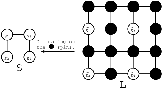
Figure 9: A schematic drawing of the real-space renormalization group (decimation) for the $d=2$ $XY$ model (1) is presented. Through decimating out the spin variables indicated by the symbol $\bullet$ within the $L$ cluster, we obtain a coarse-grained lattice identical to the $S$ cluster. Imposing the scale-invariance conditions, Eqs. (31)-(33), we arrive at the fixed point (2).

References

- (1) M. A. Novotny, J. Appl. Phys. 67, 5448 (1990).
- (2) M. A. Novotny, Phys. Rev. B 46, 2939 (1992).
- (3) M. A. Novotny, in Computer Simulation Studies in Condensed Matter Physics III, edited by D. P. Landau, K. K. Mon, and H.-B. Schüttler (Springer-Verlag, Berlin, 1991).
- (4) Y. Nishiyama, Phys. Rev. E 70, 026120 (2004).
- (5) Y. Nishiyama, Phys. Rev. E 75, 011106 (2007).
- (6) M. Barmatz, I. Hahn, J. A. Lipa, and R. V. Duncan, Rev. Mod. Phys. 79, 1 (2007).
- (7) P. Butera and M. Comi, Phys. Rev. B 56, 8212 (1997).
- (8) R. Guida and J. Zinn-Justin, J. Phys. A 31, 8103 (1998).
- (9) H. Kleinert and V. I. Yukalov, Phys. Rev. E 71, 026131 (2005).
- (10) E. Burovski, J. Machta, N. Prokof’ev, and B. Svistunov, Phys. Rev. B 74, 132502 (2006).
- (11) M. Campostrini, M. Hasenbusch, A. Pelissetto, and E. Vicari, Phys. Rev. B 74, 144506 (2006).
- (12) B.V. Costa and A.S.T. Pires, J. Mag. Mag. Mat. 262, 316 (2003).
- (13) S.A. Leonel, A.C. Oliveira, B.V. Costa, and P.Z. Coura, J. Mag. Mag. Mat. 305, 157 (2006).
- (14) J. Dely, J. Strečka, and L. Čanová, cond-mat/0611212.
- (15) H. W. J. Blöte, J. R. Heringa, A. Hoogland, E. W. Meyer, and T. S. Smit, Phys. Rev. Lett. 76, 2613 (1996).
- (16) Y. Nishiyama, Phys. Rev. E 74, 016120 (2006).
- (17) H.G. Ballesteros, L.A. Fernández, V. Martín-Mayor, and A. Muñoz Sudupe, Phys. Lett. B 441, 330 (1998).
- (18) M. Hasenbusch and T. Török, J. Phys. A 32, 6361 (1999).
- (19) R. Botet, R. Jullien, and M. Kolb, Phys. Rev. B 28, 3914 (1983).
- (20) E. R. Gagliano and C. A. Balseiro, Phys. Rev. Lett. 59, 2999 (1987).
- (21) Y. Nishiyama, Phys. Rev. E 75, 051116 (2007).
- (22) J.A. Lipa, J.A. Nissen, D.A. Stricker, D.R. Swanson, and T.C.P. Chui, Phys. Rev. B 68, 174518 (2003).
- (23) A. A. Pogorelov and I. M. Suslov, JETP Lett. 86, 39 (2007).
- (24) M. Itakura, J. Phys. Soc. Jpn. 72, 74 (2003).
- (25) R. H. Swendsen, in Real-Space Renormalization, edited by T. W. Burkhardt and J. M. J. van Leeuwen (Springer-Verlag, Berlin, 1982).