Relative-Velocity-Dependent Weber-type Models in Electromagnetism

Abstract

This article reconsiders the relative-velocity-dependent approach to modeling electromagnetism that was proposed initially by Weber before data from cathode-ray-tube (CRT) experiments was available. It is shown that identifying the nonlinear, relative-velocity terms using CRT data results in a model, which not only captures standard relativistic effects in optics, high-energy particles, and gravitation, but also explains apparent discrepancies between predicted and measured energy (i) in high-energy-particle absorption experiments and (ii) in the classical $\beta$-ray spectrum of radium-E.

1 Introduction

This article develops a Weber-type, relative-velocity-dependent electromagnetism model. Relative-velocity dependence of electromagnetism models was proposed initially by Weber [1] before data from cathode-ray-tube (CRT) experiments was available. In contrast, this article develops a nonlinear relative-velocity-dependent model that is based on data from CRT experiments. This article addresses two challenges in the use of such relative-velocity-dependent models: (i) to capture both low-velocity and high velocity effects in electromagnetism; and (ii) to maintain model-invariance between inertial reference frames. The first challenge is addressed by using the nonlinearity of the proposed model to capture: (a) low-velocity effects such as the force between two current carrying wires; and (b) high-velocity effects such as the mass increase seen in CRT experiments. The second challenge, to maintain model-invariance between different inertial frames, is addressed by accounting for the relative-velocity effects in Lorentz and Maxwell’s equations. The resulting model not only captures relativistic effects in optics, high-energy particles, and gravitation but also explains apparent discrepancies between predicted and measured energy in (i) the absorption of high-energy particles in cloud chambers [2] and   (ii) the average energy determination of the $\beta$-ray spectrum using magnetic fields. [3]Ho_36

Measurements of the energy lost by high-energy electrons due to absorption in lead, by Crane and co-workers, tend to be more than $50\%$ of the expected value. [2]  Studies of possible electron scattering and potential increase in path length (through the lead) could not explain this discrepancy. [7]  The inability to resolve this discrepancy led Richardson and Kurie [8] to conclude that the cloud-chamber-absorption method is not reliable for energy measurements “even when applied by careful investigators.”  However, the discrepancy in the measured energy can be accounted for by the model presented in this article.

The proposed model also explains apparent discrepancies between predicted and measured energy in classical $\beta$-ray spectrum experiments. Ellis and Wooster [3] found the average disintegration energy of Radium E (Ra E) to be $0.344MeV$ using temperature measurements while reporting that the average energy found by Madgwick from the $\beta$-ray spectrum was $0.395MeV$; data from both approaches are presented by Ellis and Wooster. [3]  Moreover, Madgwick’s data (including the location of the spectrum’s peak) was confirmed independently by Ho and Wang. [6]  The difference in the average energy, between these two different approaches, led to the development of several correction factors for potential errors in measurements at the lower end of the $\beta$-ray spectrum for reconciling the difference. [9, 10]  In contrast, the predicted average energy of the $\beta$-ray spectrum using the proposed relative-velocity approach matches the value from temperature measurements by Ellis and Wooster [3], without the need for correction factors.

The proposed relative-velocity model has the following general form for the Lorentz force $F_{E}$ on a particle of charge $q$ due to an electric field $E$

$$F_{E}~{}=~{}\left[{\cal N}_{\bot}(v_{rel})\right]qE_{\bot}~{}+\left[{\cal N}_{\|}(v_{rel})\right]qE_{\|}$$ (1)

where $E_{\bot}$ and $E_{\|}$ are the components of the field perpendicular and parallel to the relative velocity $v_{rel}$ between the field and the particle. It is noted that ad-hoc choices of the nonlinearities (${\cal N}_{\bot},{\cal N}_{\|}$ in equation  1) are not acceptable. For example, instead of a velocity dependent increase in mass, $m=m_{0}/\sqrt{1-\frac{|v_{rel}|^{2}}{c^{2}}}$, a reduction of the Lorentz force, such as ${\cal N}_{\bot}=\sqrt{1-\frac{|v_{rel}|^{2}}{c^{2}}}$, might be considered to match the relativistic, velocity-dependent increase in mass in CRT experiments (where $c$ is the speed of light and $m_{0}$ is the rest mass). However, it is shown that such a nonlinearity is not consistent with low-speed effects such as Ampere’s law for the force between two current-carrying wires.

In this article, the form of the perpendicular nonlinearity ${\cal N}_{\bot}$ (in equation  1) is identified using: (i) the relativistic mass increase in CRT experiments; and (ii) conservation of the field’s energy density at low speeds. It is shown that the resulting form of the perpendicular nonlinearity ${\cal N}_{\bot}$ also uniquely identifies: (i) the kinetic energy of a particle; and (ii) the parallel nonlinearity ${\cal N}_{\|}$. In addition to matching the relativistic mass increase in CRT experiments (as expected, since the nonlinearity ${\cal N}_{\bot}$ is identified using CRT observations), the resulting nonlinearity expression also matches the low-speed Ampere’s law for the force between two current carrying wires. Furthermore, the resulting energy expression explains the apparent discrepancies in the measured energy in high-energy electron absorption [2] and Ra E disintegration. [4]  Moreover, it is shown that similar relative-velocity-dependent terms result in an expression for the precession of planetary orbits that matches the prediction using general relativity. [11]

The second difficulty, to find appropriate transformations to relate observations in different inertial frames, can be addressed by the proposed relative-velocity-based approach where spatial velocity distributions ($V_{E},V_{B}$) are assigned to the electrical $E$ and magnetic fields $B$. It is shown that Maxwell’s equations, when adapted to include these relative-velocity distributions, are still co-ordinate invariant. The effects of the proposed approach on the propagation of light and the explanation of optical phenomena are considered in this article. Most importantly, the relative-velocity approach models relativistic effects such as (i) the transverse Doppler effect and (ii) the convection of light by moving media (Fresnel drag). Thus, the article presents a Weber-type relative-velocity dependent modeling approach that: (i) captures relativistic effects in optics, high-energy particles, and gravitation; and (ii) explains apparent discrepancies in experimental energy measurements.

2 Relative velocity approach

In this section, the nonlinearities ${\cal N}_{\bot},{\cal N}_{\|}$ (in equation  1) are identified. Low speed effects (energy density invariance) and high speed (CRT) effects are considered in the first two subsections to identify the perpendicular nonlinearity ${\cal N}_{\bot}$, which is then used in the third subsection to identify expressions for the kinetic energy and the parallel nonlinearity ${\cal N}_{\|}$.

2.1 Energy density conservation at low speeds

In an inertial frame $O$, let velocity fields $V_{E}$ and $V_{B}$ be associated with electric field $E$ and magnetic field $B$, respectively. Then, the Lorentz force between a charged particle $q$, moving with velocity $V$, and the fields is modeled as a function of the relative velocity between the particle and the field. The main idea is that a moving electric field introduces an apparent magnetic field (and vice versa); the model maintains a constant total energy density (electric and magnetic) that is independent of the relative velocity. This subsection begins with the relative-velocity-dependent modeling of the magnetic field.

2.1.1 Low-speed, relative-velocity modeling of magnetic field

The Lorentz force on an electrical charge $q$ due to the magnetic field in terms of the relative velocity $V-V_{B}$ of the particle with respect to the field is

$$F_{B}~{}~{}=~{}q~{}(V-V_{B})\times B$$ (2)

Thus, the magnetic field $B$ appears to have an effective electric field $E_{B}$, perpendicular to the relative velocity $V-V_{B}$, given by

$$E_{B}~{}~{}=~{}(V-V_{B})\times B$$ (3)

This apparent electric field implies that the field energy would vary with the relative velocity of the charged particle in the same reference frame. To avoid such variation, a reduction of the apparent magnetic field $B_{B}$ in the perpendicular direction is considered so that the net energy of the apparent fields is independent of the relative velocity. In particular, it is assumed that the effective magnetic field (acting on an ideal magnetic particle that is moving with velocity $V$ according to observer $O$) is given by

$$B_{B}~{}~{}=~{}B_{\|}~{}+\gamma_{B}B_{\bot}$$ (4)

where $\gamma_{B}B_{\bot}$ is the vector component of magnetic field perpendicular to the relative velocity $(V-V_{B})$, and $B_{\|}$ is the vector component of the magnetic field parallel to relative velocity $(V-V_{B})$. In the nominal case, when the relative velocity is zero, i.e., $V=V_{B}$, we have no change in the perpendicular component and therefore, $\gamma_{B}=1$ for this case. When the relative velocity is nonzero, the factor $\gamma_{B}$ is chosen such that the net energy density of $B_{B}$ and $E_{B}$ (due to the magnetic field $B$) is independent of the relative velocity $(V-V_{B})$. Moreover, the only variations in the fields are in the perpendicular components. Therefore, by matching the energy density in the field’s perpendicular component for the case when relative velocity is nonzero to the case when the relative velocity is zero, one obtains

$$\frac{\gamma_{B}^{2}}{2\mu}|B_{\bot}|^{2}~{}+\frac{\epsilon}{2}|E_{B}|^{2}~{}=~{}\frac{1}{2\mu}|B_{\bot}|^{2}$$ (5)

where $|\cdot|$ represents the magnitude of a vector, $\epsilon$ is the permittivity, and $\mu$ is the permeability. Substituting for the apparent electric field $E_{B}$ from equation  (3), i.e.,

$$E_{B}~{}=~{}(V-V_{B})\times B~{}~{}=(V-V_{B})\times B_{\bot},$$ (6)

into equation (5), yields

$$\frac{\gamma_{B}^{2}}{2\mu}|B_{\bot}|^{2}~{}+\frac{\epsilon~{}|V-V_{B}|^{2}}{2}|B_{\bot}|^{2}~{}=~{}\frac{1}{2\mu}|B_{\bot}|^{2}$$ (7)

and

$$\gamma_{B}~{}~{}=~{}\sqrt{{{1}-\frac{|V-V_{B}|^{2}}{c^{2}}}}~{}~{}=~{}\sqrt{{{1}-\beta_{B}^{2}}}~{}~{},$$ (8)

where $c={\sqrt{1/{\epsilon}{\mu}}}$ is the speed of light and $\beta_{B}$ is the normalized relative speed

$$\beta_{B}=|V-V_{B}|/c.$$ (9)

Thus, an electric particle moving with velocity $V$ is affected by the electric field $E_{B}$; a magnetic particle moving with velocity $V$ is affected by the magnetic field $B_{B}$, and the electric field $E_{B}$ moving with velocity $V_{B}$.

2.1.2 Low-speed, relative-velocity modeling of electric field

Similar to the last subsection, an electric field $E$ appears to have an effective magnetic field $B_{E}$, perpendicular to the relative velocity $V-V_{E}$, given by

$$B_{E}~{}~{}=~{}-{\epsilon}{\mu}(V-V_{E})\times E$$ (10)

where the term $-{\epsilon}{\mu}$ is used in equation (10) to match the magnetic field produced by a current-carrying wire (Ampere’s law). In particular, if $\rho$ (charge per unit length) is flowing with velocity $v$ through a wire (which is stationary in the reference frame $O$) then the electric field $E_{\rho}$ associated with this charge, at a distance $r\hat{r}$ from the wire, is given by $E_{\rho}=[\rho/(2{\pi\epsilon}r)]\hat{r}$, where $\hat{r}$ represents a unit direction vector. Note that the velocity associated with this electric field is the velocity $v$ of the charge flowing through the wire. Therefore, from equation (10), the magnetic field $B_{\rho}$ at a distance $r\hat{r}$ from the wire is

$$\begin{array}[]{rcl}B_{\rho}&=&-({\epsilon}{\mu})~{}(0-v)\times E_{\rho}=({\epsilon}{\mu})~{}v\times E_{\rho}\\ &=&{\epsilon}{\mu}[\rho/(2{\pi\epsilon}r)]|v|~{}~{}~{}~{}\hat{v}\times\hat{r}\\ &=&[\mu I/(2{\pi}r)]~{}~{}~{}~{}\hat{v}\times\hat{r}\end{array}$$ (11)

where $I$ is the current in the wire; this is the expression for magnetic field produced by a current-carrying wire.

To keep the net energy independent of the relative velocity $V-V_{E}$, the following reduction $\gamma_{E}$ in the perpendicular direction of the apparent electric field $E_{E}$ is considered

$$E_{E}~{}~{}=~{}E_{\|}~{}+\gamma_{E}E_{\bot}$$ (12)

where $\gamma_{E}E_{\bot}$ is the vector component of electric field perpendicular to the relative velocity $(V-V_{E})$, $E_{\|}$ is the vector component of the electric field parallel to relative velocity $(V-V_{E})$, and the scaling factor $\gamma_{E}=1$ when the relative velocity is zero, i.e., $V=V_{E}$. The scaling factor $\gamma_{E}$ is obtained by equating the total energy density to the energy density of the electric field alone when the relative velocity is zero as

$${\frac{\epsilon\gamma_{E}^{2}}{2}}{|E_{\bot}|^{2}}~{}+{\frac{1}{2\mu}}{|B_{E}|^{2}}~{}=~{}{\frac{\epsilon}{2}}{|E_{\bot}|^{2}}.$$ (13)

Substituting for the apparent magnetic field $B_{E}$ from equation (10), i.e.,

$$B_{E}~{}=~{}-{\epsilon}{\mu}(V-V_{E})\times E~{}~{}=~{}-{\epsilon}{\mu}(V-V_{E})\times E_{\bot},$$ (14)

into equation (13), yields

$${\frac{\epsilon\gamma_{E}^{2}}{2}}|E_{\bot}|^{2}~{}+{\frac{\epsilon^{2}\mu^{2}~{}|V-V_{E}|^{2}}{2\mu}}|E_{\bot}|^{2}~{}=~{}\frac{\epsilon}{2}|E_{\bot}|^{2}$$ (15)

and a scaling factor

$$\gamma_{E}~{}~{}=~{}\sqrt{{{1}-\frac{|V-V_{E}|^{2}}{c^{2}}}}~{}~{}.$$ (16)

This expression is similar to the one for the scaling factor for a magnetic field in equation (8). Thus, a magnetic particle moving with velocity $V$ is affected by the magnetic field $B_{E}$; an electric particle moving with velocity $V$ is affected by the electric field $E_{E}$, and the magnetic field $B_{E}$ moving with velocity $V_{E}$. In particular, the net force on an electric particle (of charge $q$) is given by [from equations (2, 10) and (12)]

$$\begin{array}[]{rcl}F_{E}&=&q~{}(V-V_{E})\times B_{E}~{}+qE_{\|}~{}+q\gamma_{E}E_{\bot}\\ &=&q~{}(V-V_{E})\times\left\{-{\epsilon}{\mu}(V-V_{E})\times E\right\}~{}~{}+qE_{\|}~{}+q\gamma_{E}E_{\bot}\\ &=&q\frac{|V-V_{E}|^{2}}{c^{2}}E_{\bot}~{}+qE_{\|}~{}+qE_{\bot}\sqrt{{1}-\frac{|V-V_{E}|^{2}}{c^{2}}}\\ &=&q\left[\beta_{E}^{2}~{}+\sqrt{{1}-\beta_{E}^{2}}\right]E_{\bot}~{}+qE_{\|}\\ &=&q\alpha E_{\bot}~{}+qE_{\|}\end{array}$$ (17)

where the normalized relative speed $\beta_{E}$ and the scaling factor $\alpha$ are given by

$$\beta_{E}=|V-V_{E}|/c~{}~{}\mbox{and}~{}~{}\alpha=\beta_{E}^{2}~{}+\sqrt{{1}-\beta_{E}^{2}}~{}~{}.$$ (18)

When the relative velocity is small, i.e., $\beta_{E}$ is small, the scaling factor $\alpha$ in the perpendicular force component in equation (17)

$$F_{E,\bot}~{}=~{}q\alpha E_{\bot}$$

can be simplified to

$$\alpha~{}=~{}\beta_{E}^{2}~{}+\sqrt{{1}-\beta_{E}^{2}}~{}~{}~{}~{}~{}\approx~{}~{}1+\frac{1}{2}\beta_{E}^{2}~{}.$$ (19)

Therefore, the simplified force on an electric particle in equation (17) becomes

$$F_{E}~{}\approx~{}q\left(1+\frac{1}{2}\beta_{E}^{2}\right)E_{\bot}~{}+qE_{\|}$$ (20)

2.1.3 Saturation effect

The discussions in the article are limited to the case when the magnitude of the relative velocity are less than the speed of light $c$, i.e., $\beta_{E}\leq 1$ and $\beta_{B}\leq 1$. The approach can be extended to higher-relative speeds by fixing (saturating) the scaling factors to the values for the case when the relative speed equals the speed of light. For example, $\alpha$ in equation (18) is held constant for higher-relative speeds $\beta_{E}>1$ as

$$\alpha=1~{}~{}\forall~{}\beta_{E}>1.$$ (21)

Although not stated explicitly, equations are presented only for the case when $\beta_{E}\leq 1$ and $\beta_{B}\leq 1$ in the rest of the article.

2.2 High-speed effects in the relative-velocity model

The relativistic mass dependence with speed is modeled as a slip effect, where the force on the particle reduces as the relative-velocity increases. In particular, consider the augmentation of the Lorentz force on an electric particle, in equations (2,  17), with relative-velocity terms $s_{\bot}$ and $s_{\|}$ as

$$F_{B}~{}=~{}\left[s_{\bot}(\beta_{B})\right]q(V-V_{B})\times B_{\bot}\\$$ (22)

$$F_{E}~{}=~{}\left[s_{\bot}(\beta_{E})\right]q\alpha E_{\bot}~{}+\left[s_{\|}(\beta_{E})\right]qE_{\|}~{}~{}~{}=F_{E,\bot}~{}~{}+F_{E,\|}.$$ (23)

The perpendicular and parallel slip terms ($s_{\bot},s_{\|}$) are identified in this subsection.

2.2.1 Matching cathode-ray-tube (CRT) observations

Consider the forces on a charge moving with velocity $V$ perpendicular to stationary magnetic $B$ and electric $E$ fields, as in cathode-ray-tube (CRT) experiments (Thomson 1897). These forces can be written, from equations (22, 23), as

$$F_{B}~{}=~{}~{}s_{\bot}(\beta)~{}q~{}{V}\times B$$ (24)

$$F_{E}~{}=~{}s_{\bot}(\beta)~{}\alpha(\beta)~{}q~{}E$$ (25)

where $\beta~{}=\frac{|{V}|}{c}$. If the fields act on the charged CRT particle over some length $L$, then the change in velocity of the CRT particle along the application of the force during the time interval $\Delta t=L/|V|$ is given by

$$\frac{F_{B}L}{m|V|}~{}~{}{\mbox{and}}~{}~{}\frac{F_{E}L}{m|V|}$$

where $m$ is the mass of the particle (electron). Therefore, the change in angles ($\theta_{B}$ and $\theta_{E}$) of the CRT particle’s path along the action of the fields $B$ and $E$, respectively, can be approximated by using equations (24, 25) as [12]

$$\theta_{B}~{}~{}=~{}|\frac{F_{B}L}{m|V|^{2}}|~{}=~{}\frac{s_{\bot}(\beta)~{}q~{}{|V|}~{}|B|~{}L}{m|V|^{2}}~{}~{}~{}=~{}\frac{s_{\bot}(\beta)~{}|B|~{}L}{\frac{m}{q}|V|}$$ (26)

$$\theta_{E}~{}~{}=~{}|\frac{F_{E}L}{m|V|^{2}}|~{}=~{}\frac{s_{\bot}(\beta)~{}\alpha(\beta)~{}|E|~{}L}{\frac{m}{q}|V|^{2}}$$ (27)

In the absence of the relative-velocity terms (i.e., $s_{\bot}(\beta)=1$ and $\alpha(\beta)=1$), a velocity-dependent mass variation can be used to explain the CRT data. In particular, the estimated velocity $V_{CRT}$ and the estimated mass-to-charge ratio

$$\frac{m(\beta_{CRT})}{q}=\frac{m}{q}~{}\Psi(\beta_{CRT}),$$

with

$$\beta_{CRT}=\frac{|{V_{CRT}}|}{c},$$ (28)

from the CRT experiments would be related by

$$\theta_{B}~{}=~{}\frac{|B|~{}L}{\frac{m}{q}\Psi(\beta_{CRT})|V_{CRT}|}$$ (29)

$$\theta_{E}~{}=~{}\frac{~{}|E|~{}L}{\frac{m}{q}\Psi(\beta_{CRT})|V_{CRT}|^{2}}$$ (30)

where $\Psi(\beta_{CRT})$ represents the CRT-predicted variation of mass with velocity. Dividing equations (26) and (27) by equations (29) and (30), respectively, yields

$$s_{\bot}(\beta)~{}=~{}\frac{|V|}{|V_{CRT}|}~{}\frac{1}{\Psi(\beta_{CRT})}$$ (31)

$$s_{\bot}(\beta)~{}\alpha(\beta)~{}=~{}\frac{|V|^{2}}{|V_{CRT}|^{2}}~{}\frac{1}{\Psi(\beta_{CRT})}.$$ (32)

The velocity $V_{CRT}$ predicted by the CRT-experiments can be obtained by dividing equation (31) by equation (32) to obtain

$$|V_{CRT}|=\frac{|V|}{\alpha(\beta)}~{}~{}~{}{\mbox{or}}~{}~{}\beta_{CRT}=\frac{\beta}{\alpha(\beta)}.$$ (33)

Furthermore, the perpendicular-slip term $s_{\bot}(\beta)$ can be found by dividing the square of equation (31) by equation (32) and then substituting for $\beta_{CRT}$ from equation (33) to obtain

$$s_{\bot}(\beta)=\frac{\alpha(\beta)}{\Psi(\beta_{CRT})}~{}~{}=\frac{\alpha(\beta)}{\Psi(\frac{\beta}{\alpha(\beta)})}.$$ (34)

Case 1: matching the relativistic mass-velocity relation:  The perpendicular term $s_{\bot}(\beta)$ can be chosen, as in equation (34), to exactly match the observed velocity-dependent variation $\Psi$ in mass. In particular, if the CRT-predicted mass increase is given by the relativistic expression

$$\Psi(\beta_{CRT})=\frac{1}{\sqrt{1-\beta_{CRT}^{2}}},$$ (35)

then the expression for the slip term $s_{\bot}$ is obtained, from equation (33) and equation (34), as

$$\begin{array}[]{rcl}s_{\bot}(\beta)&=&\alpha(\beta)~{}~{}\left\{\sqrt{1-\left[\frac{\beta}{\alpha(\beta)}\right]^{2}}\right\}\\ &=&\sqrt{\left[\alpha(\beta)\right]^{2}-\beta^{2}}\end{array}$$ (36)

Case 2: simplified perpendicular slip term:  Consider the following, simplified expression $\bar{s}_{\bot}$ for the slip term $s_{\bot}(\beta)$

$$\bar{s}_{\bot}(\beta)~{}=~{}{\left[{1~{}-\beta^{8}}\right]^{1/4}}$$ (37)

This term does not lead to an exact match of the relativistic mass increase; however, it closely approximates the expression for the relativistic mass increase. In particular, assuming this form $\bar{s}_{\bot}(\beta)$ for the slip term, the velocity $\bar{\beta}_{CRT}$ estimated in the CRT experiment, as in equation (33), is given by

$$\bar{\beta}_{CRT}~{}=~{}\frac{\beta}{\alpha(\beta)}~{}~{}=~{}\frac{\beta}{\beta^{2}+\sqrt{1-\beta^{2}}}.$$ (38)

Moreover, the apparent mass variation $\bar{\Psi}$ in the CRT experiment, as in equation (34), is given by

$$\bar{\Psi}(\bar{\beta}_{CRT})~{}=~{}\frac{\alpha(\beta)}{s(\beta)}~{}~{}=~{}\frac{\beta^{2}+\sqrt{1-\beta^{2}}}{\left[{1~{}-\beta^{8}}\right]^{1/4}}.$$ (39)

It is noted that the variation of $\bar{\Psi}(\bar{\beta}_{CRT})$ with velocity $\bar{\beta}_{CRT}$ in equations (38, 39), which would be obtained from a CRT experiment, is similar to the relativistic variation

$$\Psi(\bar{\beta}_{CRT})=\frac{1}{\sqrt{1-\bar{\beta}_{CRT}^{2}}}$$ (40)

as shown in figure 1.

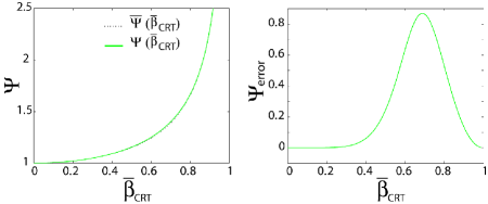
Figure 1: Proposed model matches the apparent velocity dependence of mass in CRT experiments. Left plot: comparison of apparent mass variations ${\Psi}(\bar{\beta}_{CRT})$ (relativistic mass model) and $\bar{\Psi}(\bar{\beta}_{CRT})$ (simplified model) as in Eqs. (39, 40) with normalized relative speed $\bar{\beta}_{CRT}$ in Eq. (38). Right plot: the difference $\Psi_{error}$ in predicted mass variation is less than 1% with the simplified model in Eq. (41). An match would have no error with the exact relative-velocity model in Eq. (36).

Moreover, the percentage difference $\Psi_{error}$ between the two expressions (equations 39 and 40) given by

$$\Psi_{error}=\frac{{\Psi}(\bar{\beta}_{CRT})-\bar{\Psi}(\bar{\beta}_{CRT})}{\Psi(\bar{\beta}_{CRT})}\times 100$$ (41)

is less than $1\%$ as shown in figure 1. Thus, the relativistic velocity dependency of mass in CRT experiments can be modeled using the relative-velocity approach with the perpendicular nonlinearity (${\cal N}_{\bot}=s_{\bot}\alpha$) in the Lorentz force expression and a constant mass. The simplified expression for the perpendicular slip ($s_{\bot}=\bar{s}_{\bot}$ with $\bar{s}_{\bot}$ defined in Eq. 37) is used in the rest of the article.

2.3 Kinetic energy and parallel slip

The expressions for kinetic energy ${{\cal{E}}_{KE}}$ and the parallel slip term ${s}_{\|}$ are identified in this subsection by using the perpendicular slip term ${s}_{\bot}$ .

2.3.1 Relationship between parallel slip and kinetic energy

Consider a charged particle $q$ moving along a straight line away from a stationary charged particle $Q$ at a distance $r\hat{r}$ as shown in figure 2 (case 1).

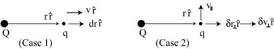
Figure 2: Two cases: (i) forces parallel; and (ii) forces perpendicular to the velocity.

Taking the dot product with a small displacement $dr\hat{r}$ with Newton’s law on the charge $q$ yields

$$s_{\|}(\beta)\frac{Qq}{4\pi\epsilon r^{2}}dr~{}~{}=~{}m\frac{dv}{dt}dr~{}~{}=\frac{m}{2}dv^{2}~{}~{}=\frac{mc^{2}}{2}d\beta^{2}.$$ (42)

Dividing both sides by the parallel slip term $s_{\|}(\beta)$ and integrating results in

$$\int_{r_{1}}^{r_{2}}\frac{Qq}{4\pi\epsilon r^{2}}dr = \int_{\beta^{2}_{1}}^{\beta^{2}_{2}}\frac{mc^{2}}{2s_{\|}(\beta)}d\beta^{2}~{}~{}=\int_{{\cal{E}}_{KE,1}}^{{\cal{E}}_{KE,2}}\frac{d{\cal{E}}_{KE}}{d\beta^{2}}d\beta^{2}$$ (43)

where ${\cal{E}}_{KE}$ is considered as the relative-velocity dependent kinetic energy of the system since the above expression leads to the conservation law

$$\frac{Qq}{4\pi\epsilon r_{2}}+{\cal{E}}_{KE,2}~{}~{}=\frac{Qq}{4\pi\epsilon r_{1}}+{\cal{E}}_{KE,1}$$ (44)

in which the potential energy expression ${Qq}/({4\pi\epsilon r})$ is independent of the relative velocity and the parallel slip term $s_{\|}(\beta)$. The relationship between the parallel slip term and the kinetic energy is (from equation 43)

$$\frac{d{\cal{E}}_{KE}}{d\beta^{2}}~{}~{}=~{}\frac{mc^{2}}{2s_{\|}(\beta)}.$$ (45)

2.3.2 Expression for kinetic energy

The perpendicular force $F_{E,\bot}$ does zero work and therefore does not lead to changes in the kinetic energy. However, an expression for kinetic energy can be found by making the virtual work done by the perpendicular force $F_{E,\bot}$ independent of the perpendicular slip term $s_{\bot}$. Consider a charged particle $q$ moving with velocity $v_{\|}$ perpendicular to the distance vector $r\hat{r}$ from a stationary charged particle $Q$ as shown in figure 2 (case 2). Let $\delta{r_{\bot}}\hat{r}$ be a virtual displacement perpendicular to the relative velocity $v_{\|}$; then taking the dot product of the virtual displacement with both sides of Newton’s law yields

$$s_{\bot}(\beta_{\|})\alpha(\beta_{\|})\frac{Qq}{4\pi\epsilon r^{2}}\delta{r_{\bot}}~{}~{}=~{}~{}m\frac{\delta{v_{\bot}}}{\delta{t}}\delta{r_{\bot}}~{}~{}~{}=mv_{\bot}\delta{v_{\bot}}~{}~{}~{}=\frac{1}{2}m~{}\delta{v_{\bot}^{2}}~{}$$ (46)

where $\beta_{\|}=\frac{|v_{\|}|}{c}$. The virtual work done can be made independent of the slip term $s_{\bot}(\beta_{\|})$ if the change in the kinetic energy ($\delta{{\cal{E}}_{KE}}$) has the following form (obtained by dividing both sides of the above equation by $s_{\bot}(\beta_{\|})$)

$$\alpha(\beta_{\|})\frac{Qq}{4\pi\epsilon r^{2}}\delta{r_{\bot}}~{}~{}=~{}~{}\frac{1}{2}\frac{m~{}\delta{v_{\bot}^{2}}}{s_{\bot}(\beta_{\|})}~{}~{}=~{}~{}\frac{1}{2}\frac{mc^{2}~{}\delta{\beta_{\bot}^{2}}}{s_{\bot}(\beta_{\|})}~{}~{}=~{}\delta{{\cal{E}}_{KE}}$$ (47)

which implies that the kinetic energy ${{\cal{E}}_{KE}}$ has the form

$${{\cal{E}}_{KE}}(\beta)~{}~{}=~{}\frac{1}{2}\frac{mc^{2}\beta^{2}}{s_{\bot}}~{}~{}~{}~{}~{}=\frac{1}{2}\frac{mc^{2}\beta^{2}}{(1-\beta^{8})^{1/4}}.$$ (48)

2.3.3 Expression for parallel slip term

Differentiating the expression (equation 48) for the kinetic energy by $\beta^{2}$ yields

$$\frac{d{\cal{E}}_{KE}}{d\beta^{2}}~{}~{}=~{}\frac{mc^{2}}{2}\left[\frac{1}{(1-\beta^{8})^{5/4}}\right].$$ (49)

and comparison with equation (45) yields the parallel slip term as

$$s_{\|}~{}~{}=~{}(1-\beta^{8})^{5/4}.$$ (50)

2.4 Summary of relative-velocity-dependent model

The relative velocity approach results in the following Lorentz force on an electrically charged particle (from equation 22 and equation 23) by using the simplified slip terms (in equation 37 and equation 50)

$$F_{B}~{}=~{}\left[(1-\beta_{B}^{8})^{1/4}\right]q(V-V_{B})\times B_{\bot}$$ (51)

$$F_{E}~{}=~{}\left[(1-\beta_{E}^{8})^{1/4}\right]\left[\sqrt{1-\beta_{E}^{2}}+\beta_{E}^{2}\right]qE_{\bot}~{}+\left[(1-\beta_{E}^{8})^{5/4}\right]qE_{\|}.$$ (52)

where the electrical force expression (in equation 52) reduces to the expression in equation (20) at low speeds.

3 Applications of Lorentz force expression

In this section, it is shown that relative-velocity-dependent Lorentz force expression: (a) satisfies the force between two wires (a low-velocity effect); and (b) explains the observed discrepancy in the energy of high-velocity particles. Moreover, it is shown that similar relative-velocity dependence of the gravitational force can explain the excess precession in planetary orbits.

3.1 Force between two wires

The increase in the electrical force component perpendicular to the relative velocity [in equation (52) which simplifies to equation (20) at low speeds] can be used to explain the force between two current carrying wires, which are both stationary in a reference frame $O$. As shown in figure 3, let the second wire (denoted by the subscript 2) be positioned at $r\hat{r}$ from the first wire (denoted by the subscript 1). Moreover, let the currents in the two parallel wires be $I_{1}$ and $I_{2}$, and let the corresponding moving charges (per unit length) be $-\rho_{1}$ and $-\rho_{2}$ with velocities $-v_{1}\hat{V}$ and $-v_{2}\hat{V}$, respectively, i.e.,

$$I_{1}=\rho_{1}v_{1},~{}{\mbox{and}}~{}I_{2}=\rho_{2}v_{2}$$ (53)

where the speeds $v_{1}\geq 0$ and $v_{2}\geq 0$ of the charges are small, and $\hat{V}$ is a unit vector along the direction of the wire (in which current is flowing).

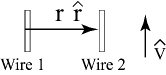
Figure 3: Force between two current carrying parallel wires separated by distance $r$.

3.1.1 Force expression

Consider the two (non-canceling) fields in the first wire: (a) $E_{-\rho_{1}}$ associated with the moving charge $-\rho_{1}$ with field velocity $-v_{1}\hat{V}$ given by

$$E_{-\rho_{1}}=[-\rho_{1}/(2{\pi\epsilon}r)]\hat{r};$$ (54)

and (b) $E_{\rho_{1}}$ associated with the corresponding stationary charge $\rho_{1}$ in the wire, i.e., the stationary field given by

$$E_{\rho_{1}}=[\rho_{1}/(2{\pi\epsilon}r)]\hat{r}.$$ (55)

These two fields act on the moving charge $-\rho_{2}$ and a corresponding stationary charge $\rho_{2}$ on the second wire (per unit length). For example, the force per unit length $F_{-\rho_{1},-\rho_{2}}$ on the moving charge $-\rho_{2}$ due to the moving charge $-\rho_{1}$ can be obtained from equations (20, 54) as

$$\begin{array}[]{rcl}F_{-\rho_{1},-\rho_{2}}&=&-\rho_{2}\left(1+\frac{|(-v_{2})-(-v_{1})|^{2}}{2c^{2}}\right)E_{-\rho_{1}}\\ &=&-\rho_{2}\left(1+\frac{|(-v_{2})-(-v_{1})|^{2}}{2c^{2}}\right)[-\rho_{1}/(2{\pi\epsilon}r)]\hat{r}\\ &=&\frac{\rho_{1}\rho_{2}\hat{r}}{2{\pi\epsilon}r}\left(1+\frac{|v_{1}-v_{2}|^{2}}{2c^{2}}\right).\end{array}$$ (56)

Similarly, (i) the force per unit length $F_{\rho_{1},-\rho_{2}}$ on the moving charge $-\rho_{2}$ due to the stationary charge $\rho_{1}$, as well as (ii) the the forces $F_{-\rho_{1},\rho_{2}},F_{\rho_{1},\rho_{2}}$ on the stationary charge $\rho_{2}$ on the second wire due to the charges (on the first wire) $-\rho_{1}$ and $\rho_{1}$, respectively, are given by

$$\begin{array}[]{rcl}F_{\rho_{1},-\rho_{2}}&=&-\frac{\rho_{1}\rho_{2}\hat{r}}{2{\pi\epsilon}r}\left(1+\frac{|-v_{2}|^{2}}{2c^{2}}\right)\\ F_{-\rho_{1},\rho_{2}}&=&-\frac{\rho_{1}\rho_{2}\hat{r}}{2{\pi\epsilon}r}\left(1+\frac{|v_{1}|^{2}}{2c^{2}}\right)\\ F_{\rho_{1},\rho_{2}}&=&\frac{\rho_{1}\rho_{2}\hat{r}}{2{\pi\epsilon}r}~{}.\end{array}$$ (57)

Thus, the total force per unit length $F_{1,2}$ on the second wire can be found using equations (56, 57) as

$$\begin{array}[]{rcl}F_{1,2}&=&F_{\rho_{1},\rho_{2}}+F_{\rho_{1},-\rho_{2}}+F_{-\rho_{1},\rho_{2}}+F_{-\rho_{1},-\rho_{2}}\\ &=&\frac{\rho_{1}\rho_{2}\hat{r}}{2{\pi\epsilon}r}\left[{1-\left(1+\frac{|v_{2}|^{2}}{2c^{2}}\right)-\left(1+\frac{|v_{1}|^{2}}{2c^{2}}\right)+\left(1+\frac{|v_{1}-v_{2}|^{2}}{2c^{2}}\right)}\right]\\ &=&\frac{\rho_{1}\rho_{2}\hat{r}}{2{\pi\epsilon}r}~{}\left(\frac{-2v_{1}v_{2}}{2c^{2}}\right)~{}~{}=~{}-\frac{\mu I_{1}I_{2}}{2{\pi}r}\hat{r}.\end{array}$$ (58)

This force on the second wire is attractive (i.e., towards the first wire) when the two wires carry current in the same direction.

3.1.2 Force between wires is incorrect with ad-hoc perpendicular slip term

Another choice of the perpendicular slip term can be found by matching the acceleration resulting from the relativistic increase in mass with speed. For example, the slip term $s_{\bot}(\beta_{E})$ in equation (23) can be chosen such that the perpendicular component of the force due to an electric field becomes

$$F_{E,\bot}~{}=~{}~{}\left[s_{\bot}(\beta_{E})\right]q\alpha E_{\bot}~{}~{}=qE_{\bot}\sqrt{1-\beta_{E}^{2}}.$$ (59)

The resulting force can be approximated (at low speeds $\beta_{E}$) by

$$F_{E,\bot}~{}\cong~{}~{}qE_{\bot}\left(1-\frac{\beta_{E}^{2}}{2}\right).$$ (60)

However, this expression is not consistent with the force between two current carrying wires. In particular, the scaling of the term $\beta_{E}^{2}$ has the opposite sign in equation (60) when compared to the expression in equation (20). The use of the expression in equation (60) would lead to a force

$$F_{1,2}~{}=\frac{\mu I_{1}I_{2}}{2{\pi}r}\hat{r}$$ (61)

similar to equation (58); however, the force between two wires that are carrying current in the same direction is repulsive, which is incorrect.

3.2 High-velocity particles

The energy and velocity of charged particles in magnetic fields predicted by the relative velocity approach are compared with relativistic predictions. These are then used to explain apparent discrepancies in the measured energy of high-velocity experiments.

3.2.1 Comparison of energy and velocity expressions

The motion of a particle with charge $q$ and mass $m$ moving with speed $v$ in a magnetic field $B$ along a circle with radius $\rho$ is governed by

$$\frac{mv^{2}}{\rho}~{}=~{}qvs_{\bot}B~{}~{}~{}~{}~{}{\mbox{i.e.,}}~{}~{}\frac{\beta}{(1-\beta^{8})^{1/4}}~{}~{}=~{}\left(\frac{q}{mc}\right)\rho B~{}~{}=\kappa.$$ (62)

The relativistic expression for velocity $v_{r}$ (and $\beta_{r}=|v_{r}|/c$), for a given value of the non-dimensional parameter $\kappa$, can be found as

$$\frac{mv_{r}^{2}}{\rho\sqrt{1-\beta_{r}^{2}}}~{}=~{}qv_{r}B~{}~{}~{}~{}~{}{\mbox{i.e.,}}~{}~{}\frac{\beta_{r}}{(1-\beta_{r}^{2})^{1/2}}~{}~{}=\kappa$$ (63)

where $m$ represents the rest mass in relativity. The corresponding relativistic energy ${\cal{E}}_{r}$ is given by

$${{\cal{E}}_{r}}~{}=~{}\frac{mc^{2}}{(1-\beta_{r}^{2})^{1/2}}-mc^{2}$$ (64)

while the relative-velocity-based energy ${\cal{E}}$ is given by equation (48). The predicted velocity and energy for the relative velocity approach are compared with those from the relativistic expressions in figure 4.

Figure 4: Variation of normalized speed (left plot) and energy (right plot).

Note that the velocity $\beta$ predicted by the relative velocity approach tends to be higher than the relativistic value $\beta_{r}$ while the energy ${\cal{E}}$ predicted by the relative velocity approach tends to be lower than the relativistic value ${{\cal{E}}_{r}}$ for large values of $\kappa$. This difference is used to explain (below) the discrepancies in the observed energy in absorption experiments and in the $\beta$-ray spectrum.

3.2.2 Absorption of high-energy electrons

Crane and co-workers [2] investigated the absorption of high-energy electrons in lead by measuring the initial energy ${{\cal{E}}_{i,r}}$ and final energy ${{\cal{E}}_{f,r}}$ of electrons before and after passing through a lead absorber in a cloud chamber. [2]  The subscript $r$ denotes that the relativistic expression is used to find the energy from the measured curvature in a magnetic field. The corresponding initial and final energy, from the relative-velocity approach, are found from figure 5 plot(a) which plots the energy from the relative-velocity approach against the corresponding relativistic energy at different radii in the magnetic field (i.e., different $\kappa$). Data from Crane’s results (Turin and Crane, [2]  figure 7) is used to recompute the energy loss using the relative velocity approach — the results are shown in Table 1 and in figure 5 plot(b) which plots the energy loss $\Delta{{\cal{E}}}={{\cal{E}}_{i}}-{{\cal{E}}_{f}}$ versus the average energy ${\bar{\cal{E}}}=({{\cal{E}}_{i}}-{{\cal{E}}_{f}})/2$.

Relativity approach				Relative velocity
average	loss	initial	final	initial	final	average	loss
${\bar{\cal{E}}_{r}}$	$\Delta{{\cal{E}}_{r}}$	${{\cal{E}}_{r,i}}$	${{\cal{E}}_{r,f}}$	${{\cal{E}}_{i}}$	${{\cal{E}}_{f}}$	${\bar{\cal{E}}}$	$\Delta{{\cal{E}}}$
Mev	Mev/cm	Mev	Mev	Mev	Mev	Mev	Mev/cm
2.27	28.5	2.983	1.558	1.728	1.002	1.365	14.424
4.12	33	4.945	3.295	2.716	1.886	2.301	16.606
4.12	35	4.995	3.245	2.741	1.861	2.301	17.613
5.85	43.5	6.938	4.763	3.716	2.624	3.170	21.823
8.35	45.5	9.488	7.213	4.993	3.853	4.423	22.789

Table 1: Re-evaluation of energy loss in electron absorption from data by Turin and Crane. [2]   Thickness of the lead absorber is $0.5mm$. [2]

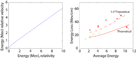
Figure 5: Relative-velocity-based energy vs. relativistic energy in magnetic fields (left plot). Right plot: the large deviation between predicted and experimental energy loss $\Delta{{\cal{E}}}$ for different average energy ${\bar{\cal{E}}}$ is avoided with the relative-velocity-based approach. The relative-velocity-based values (circles) are from Table 1; the relativity-based values (solid dots) and the theoretical curves (solid/dashed lines) are from Turin and Crane [2], figure 7.

Thus, the results show that the large deviation (more than 50% increase) in the energy loss from the theoretical prediction (Turin and Crane, [2]  figure 7) when energy is computed with the relativistic approach is avoided when the data is re-interpreted with the relative-velocity-based expression for energy.

3.2.3 Average energy of $\beta$-ray spectrum

Ellis and Wooster [3] found the average disintegration energy of Radium E (Ra E) to be $0.344MeV$ using temperature measurements while the average energy found from the $\beta$-ray spectrum in magnetic fields (Ellis and Wooster [3], figure 1) was $0.395MeV$. The resulting spectrum [3] is shown in figure 6 (solid line); data points were measured on this curve and the corresponding relative-velocity based energy was found using the same relationship in figure 5(plot a) — the recomputed data points are also shown in figure 6.

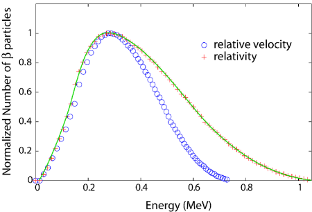
Figure 6: $\beta$-particle counts vs energy. The relative-velocity approach predicts a reduction in the number of particles at the high-energy end of the spectrum; the resulting average energy is closer to the temperature-based measurement by Ellis and Wooster. [3]  The solid line is Madgwick’s curve (from Ellis and Wooster, [3]   Fig. 1) with the relativistic energy expression. The crosses are data points obtained from the solid curve; these data points are used to find the corresponding relative-velocity-based energy (circles).

Note that the value of the energy is smaller for the relative-velocity approach when compared to the relativistic energy (towards the higher end of the spectrum in figure 6); therefore, the average energy is smaller with the relative-velocity approach. The average value of the spectrum with the relativistic data points is $0.39Mev$ while the average value of the spectrum with the relative-velocity-based points is $0.35Mev$. Thus, the re-computed average energy ($0.35Mev$) of Madgwick’s $\beta$-ray spectrum data is close to the average ($0.344Mev$) obtained by Ellis and Wooster [3] using temperature measurements when compared to the value of $0.39Mev$ with the relativistic energy expression [3]. Therefore, the apparent discrepancy in Madgwick’s data [3] can be explained by using the relative-velocity-based approach.

3.3 Precession of planetary orbits

It is shown that relative-velocity dependence of the normal force can be used to explain the additional precession in planetary orbits.

3.3.1 Gravitational force expression with slip terms

Consider a similar nonlinearity (as in equation 52) for modeling the gravitational force on a planet of mass $m_{p}$

$$F_{G} = s_{\bot}(\beta)\left[\alpha_{G}(\beta)\right]m_{p}G_{\bot}~{}+s_{\|}(\beta)m_{p}G_{\|}~{}~{}~{}=F_{G,\bot}~{}+F_{G,\|}$$ (65)

where $G_{\|}$ and $G_{\bot}$ represents the gravitational field components due to the sun (mass $M_{s}$) that are parallel and perpendicular to the relative velocity $v_{rel}$ with respect to the gravitational field and $\beta=|v_{rel}|/c$. If the expression for kinetic energy is kept the same for gravitational fields as with electrical or magnetic fields, then the slip terms ($s_{\bot},s_{\|}$) will be the same for gravitational fields. However, there is still flexibility in the choice of the term $\alpha_{G}(\beta)$ in the normal force.

3.3.2 Perturbation of the potential

For planetary orbits, the speeds are small (therefore $\beta^{8}$ is small and the slip terms are close to one), and the orbits are almost circular hence the central force is close to the normal force $F_{G,\bot}$. Therefore, the gravitational force on the planet (in equation 65) at a distance $r\hat{r}$ from the sun can be approximated by the normal force given by

$$F_{G} = -G\frac{m_{p}M_{s}}{r^{2}}\left[\alpha_{G}(\beta)\right]\hat{r}~{}~{}=-G\frac{m_{p}M_{s}}{r^{2}}\left[1+K_{G}{\beta^{2}}\right]\hat{r}$$ (66)

where $G$ is the gravitational force constant, $m_{p}$ is the mass of the planet, $M_{s}$ is the mass of the sun, and $K_{G}$ is a constant. Energy conservation (obtained using the same integration procedure used to obtain equation 44) with the kinetic energy expression in equation (48) at low speeds yields

$$-G\frac{m_{p}M_{s}}{r}+\frac{1}{2}\frac{m_{p}c^{2}\beta^{2}}{(1-\beta^{8})^{1/4}}~{}~{}\approx~{}-G\frac{m_{p}M_{s}}{r}+\frac{1}{2}{m_{p}c^{2}\beta^{2}}~{}={\cal{E}}$$ (67)

where ${\cal{E}}$ is a constant — the total energy at any point on the orbit. Substituting for $\beta^{2}=\frac{2\cal{E}}{m_{p}c^{2}}+G\frac{2M_{s}}{rc^{2}}$ from equation (67) into equation (66) results in a force expression

$$F_{G} = -G\frac{m_{p}M_{s}(1+\frac{2K_{G}\cal{E}}{m_{p}c^{2}})}{r^{2}}\hat{r}~{}-2K_{G}G^{2}\frac{m_{p}M_{s}^{2}}{c^{2}r^{3}}\hat{r}$$ (68)

and an associated potential-like function $V(r)$ such that $F_{G}(r)=-\nabla V(r)$ given by

$$V = -\frac{Gm_{p}M_{s}(1+\frac{2K_{G}\cal{E}}{m_{p}c^{2}})}{r}~{}-\frac{K_{G}G^{2}m_{p}M_{s}^{2}}{c^{2}r^{2}}$$ (69)

$$= -\frac{Gm_{p}M_{s}(1+\frac{2K_{G}\cal{E}}{m_{p}c^{2}})}{r}~{}-\frac{h}{r^{2}}$$

where $h=\frac{K_{G}G^{2}m_{p}M_{s}^{2}}{c^{2}}$ and the $1/r$ potential is perturbed by $-{h}/{r^{2}}$.

3.3.3 Precession due to perturbation of the potential

The precession rate $\dot{P}$ for a perturbation of the potential ($V$) with the form $-h/r^{2}$ is equal to (see Goldstein, [11]  equations (11-46 and 11-50))

$$\dot{P}=\frac{2\pi h}{GM_{s}m_{p}a(1-\epsilon^{2})T_{p}}~{}~{}=~{}\frac{2\pi K_{G}GM_{s}}{a(1-\epsilon^{2})T_{p}c^{2}}$$ (70)

where $T_{p}$ is orbital time period, $a$ is the semi-major axis and $\epsilon$ is the eccentricity of the orbit. This matches the general relativistic prediction of precession rate given by (see Goldstein, [11]  equations (11-51 and 11-52))

$$\dot{P}~{}=~{}\frac{6\pi GM_{s}}{a(1-\epsilon^{2})T_{p}c^{2}}$$ (71)

when the constant $K_{G}=3$. It is noted that the term $(1+\frac{2K_{G}\cal{E}}{m_{p}c^{2}})$ is approximately one in equations (68, 69) since $\frac{2K_{G}\cal{E}}{m_{p}c^{2}}$ is of the order $10^{-8}$ and is negligible. The resulting gravitational force expression is

$$F_{G} = \left[(1-\beta^{8})^{1/4}\right]\left[1+3\beta^{2}\right]m_{p}G_{\bot}~{}+\left[(1-\beta^{8})^{5/4}\right]m_{p}G_{\|}$$ (72)

Thus, the relative-velocity dependent approach can predict the excess precession of planetary orbits.

4 Optics

The field velocities ($V_{E},V_{B}$) introduce extra terms in Maxwell’s equations that are removed to retain co-ordinate invariance. It is shown that the proposed model captures relativistic effects in: (i) the propagation speed of light; (ii) stellar aberration; (iii) the transverse Doppler effect; and (iv) the convection of light by moving media.

4.1 Relative-velocity in Maxwell’s equations

Consider an electric $E$ and a magnetic $M$ field, which are stationary with respect to an inertial frame $O_{1}$, and satisfy Maxwell’s equations in free space without charges

$$\nabla\times E~{}=~{}-\frac{{\partial}B}{{\partial}t}$$ (73)

$$\nabla\times B~{}=~{}\epsilon\mu\frac{{\partial}E}{{\partial}t}.$$ (74)

Consider the same equation in a different inertial frame $O_{2}$ in which the inertial frame $O_{1}$ is moving with constant velocity $V$. The Galilean transformation between the two frames

$$X_{2}=X_{1}+Vt$$

gives the following relations at any location ($X_{1}$ in frame $O_{1}$ or $X_{2}-Vt$ in frame $O_{2}$)

$${\mbox{Frame}}~{}O_{1} {\mbox{Frame}}~{}O_{2}$$ (75)

$$E(a,b),~{}~{}B(a,b) E(a,b),~{}~{}B(a,b)$$ (76)

$$a=X_{1},~{}~{}b=t, a=X_{2}-Vt,~{}~{}b=t$$ (77)

$$V_{E}=0,~{}~{}V_{B}=0 V_{E}=V,~{}~{}V_{B}=V$$ (78)

$$\frac{{\partial}E}{{\partial}t}=\frac{{\partial}E}{{\partial}b} \frac{{\partial}E}{{\partial}t}=\frac{{\partial}E}{{\partial}a}(-V_{E})~{}+\frac{{\partial}E}{{\partial}b}$$ (80)

$$~{}~{}~{}~{}~{}=-(V_{E}\cdot\nabla)E~{}+\frac{{\partial}E}{{\partial}b}$$

$$\frac{{\partial}E}{{\partial}X_{1}}=\frac{{\partial}E}{{\partial}a} \frac{{\partial}E}{{\partial}X_{2}}=\frac{{\partial}E}{{\partial}a}.$$ (81)

Since the spatial gradient is invariant with frame, in equation (81), the curl — e.g., $\nabla\times B$ on the left hand side of equation (74) — is also frame invariant. However, the partial time derivative in equation (80) has an extra term in frame 2. Therefore, the partial derivative with time, such as $\frac{{\partial}E}{{\partial}t}$ on the right hand side of equation (74), has an extra term $-(V_{E}\cdot\nabla)E$. Hence, adding the term $(V_{E}\cdot\nabla)E$ to Maxwell’s equation (74) will make it frame invariant under the relative-velocity-dependent approach; the modified equation becomes

$$\nabla\times B~{}=~{}\epsilon\mu\left(\frac{{\partial}E}{{\partial}t}~{}+(V_{E}\cdot\nabla)E\right).$$ (82)

Noting that

$$\frac{dE}{dt}~{}=~{}\frac{{\partial}E}{{\partial}t}~{}+(V_{E}\cdot\nabla)E$$ (83)

and using a similar argument to modify equation (73), we obtain the following inertial-frame invariant form of Maxwell’s equations with terms that include the field velocities ($V_{E},V_{B}$)

$$\nabla\times E~{}=~{}-\frac{dB}{dt}$$ (84)

$$\nabla\times B~{}=~{}\epsilon\mu\frac{dE}{dt}$$ (85)

4.1.1 Invariance with co-ordinate change

Electric $E$ and magnetic $B$ fields, with field velocities $V_{E}$ and $V_{B}$, respectively, that satisfy Maxwell’s equations in one reference frame also satisfy it in another inertial reference frame with a Galilean transformation of the field velocities. In this sense, the modified Maxwell’s equations [equations (84), (85)] with the total time derivatives are invariant to Galilean transformations between inertial reference frames.

4.1.2 Addition of current density

It is noted that a current density of the form

$$\mu J=\mu\epsilon\left({\nabla\cdot E}\right)V_{E}$$ (86)

can be added to the right hand side of equation (85) but is not needed in the following discussion on optics.

4.2 Propagation Speed of Light

Consider the following two wave equations, which are considered as disturbances on the nominal electrical $E$ and magnetic $B$ fields, each of which has a field velocity

$$V_{E}=V_{B}=V=v_{z}\hat{z},$$

with magnitude $v_{z}$ in the $\hat{z}$ direction, given by

$$E~{}=~{}e_{x}\cos{(\omega t-kz)}~{}\hat{x}$$ (87)

$$B~{}=~{}b_{y}\cos{(\omega t-kz)}~{}\hat{y}.$$ (88)

The terms in the modified Maxwell’s equations [equations (84), (85)] for the above wave equations are computed below.

$$\nabla\times B~{}=~{}-b_{y}k\sin{(\omega{t}-kz)}~{}~{}\hat{x}$$ (89)

$$\nabla\times E~{}=~{}e_{x}k\sin{(\omega{t}-kz)}~{}~{}\hat{y}$$ (90)

$$\frac{dB}{dt}~{}=~{}\left[{-\omega~{}+kv_{z}}\right]b_{y}\sin{(\omega t-kz)}~{}\hat{y}$$ (91)

$$\frac{dE}{dt}~{}=~{}\left[{-\omega~{}+kv_{z}}\right]e_{x}\sin{(\omega t-kz)}~{}\hat{x}$$ (92)

Substituting equations (89-92) into the modified Maxwell’s equations [equations (84), (85)] yields

$$e_{x}k~{}=~{}-\left[{-\omega~{}+kv_{z}}\right]b_{y}$$ (93)

$$-b_{y}k~{}=~{}\epsilon\mu\left[{-\omega~{}+kv_{z}}\right]e_{x}$$ (94)

By setting $e_{x}=b_{y}c$ and $\mu\epsilon=\frac{1}{c^{2}}$ both the equations reduce to the common expression

$$ck~{}=~{}\left({\omega~{}-kv_{z}}\right).$$ (95)

Note that the wave propagation speed $V_{light}$ is given by $\omega/k$; therefore, the light propagation speed (in the z-direction) is additive, i.e.,

$$V_{light}~{}=~{}\omega/k~{}~{}=~{}c~{}+v_{z}.$$ (96)

Thus, the modified Maxwell’s equations allow the nominal velocity of the field $V$, in which light is generated, to be added to the standard velocity of light when the field is non-moving — this follows directly from the invariance of modified Maxwell’s equations.

It is noted that the Michelson-Morley experiment is expected to yield the null result with the moving fields approach because the velocity of light is constant in all directions with respect to frame of measurements (in which light was generated).

4.3 Effect of star’s velocity on aberration

In a reference frame on earth, the velocity of the earth ${V}_{e}=v_{e}\hat{V}_{e}$ adds to the velocity of stellar light to generate the aberration effect, see equation (96), as in the original explanation by Bradley. [13]  The angle of the light direction with respect to earth ($\theta$ measured perpendicular to earth’s motion as shown in figure 7) is maximum if the star’s velocity ${V}_{s}=v_{s}\hat{V}_{s}$ reduces the nominal light speed to $c-v_{s}$ (when angle $\theta_{s}=0$). Thus, the maximum change in the light direction with respect to earth is $2\theta$ where

$$\tan{\theta}~{}=~{}\frac{v_{e}}{c-v_{s}}.$$ (97)

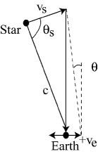
Figure 7: Aberration formula based on relative-velocity matches the classical expression [13].

For small speeds $v_{s}$ and $v_{e}$ the above expression is only linear in $v_{e}$ (and not linear in $v_{s}$) — it can be approximated as

$$\theta~{}\approx~{}\frac{v_{e}}{c}$$ (98)

The effect of the star’s velocity ${V}_{s}$ on the aberration effect (due to Earth’s motion) is small if the speed of the star is small, i.e., ${v}_{s}$ is much smaller than the nominal velocity of light $c$. Therefore, stellar aberration appears to be independent of the star’s velocity $V_{s}$ [14] and appears to only depend on the relative change in the observer’s velocity. [15]

4.4 Transverse Doppler effect

Consider the Doppler effect due to addition of velocities in different frames. Let light be generated in frame 1 with velocity $C=c\hat{C}$ and angle $\theta_{1}$ (in frame 1). Moreover, in frame 2, the observed velocity of light is $C_{2}={c}_{2}\hat{C}_{2}$ with angle $\theta_{2}$ as shown in Fig 8. Furthermore, let frame 1 be moving with relative velocity ${V}=v\hat{V}$ relative to frame 2.

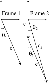
Figure 8: Relative-velocity approach explains the transverse Doppler effect: Frame 1, which has relative velocity $V$ with respect to frame 2, generates light whose velocity is $c$ in frame 1. The observed velocity of the light is at an angle $\theta_{2}$ in frame 2

The magnitude ${c}_{2}$ of the observed velocity (at an angle $\theta_{2}$) can be determined from the law of cosines

$${v}^{2}~{}+c_{2}^{2}~{}-2{v}c_{2}\cos{\theta_{2}}=c^{2}$$ (99)

which implies that

$$c_{2}~{}={v}cos{\theta_{2}}~{}+\sqrt{c^{2}~{}-{v}^{2}\sin^{2}{\theta_{2}}}.$$

Hence, the frequencies $f_{1},f_{2}$ in the two frames are related by

$$\begin{array}[]{rcl}f_{2}&=&f_{1}\frac{c_{2}}{c}\\ &=&f_{1}\frac{v\cos{\theta_{2}}+\sqrt{{c}^{2}-{v}^{2}\sin^{2}{\theta_{2}}}}{c}\\ &=&\left\{\begin{array}[]{ll}f_{1}(1+\frac{v}{c})&~{}{\mbox{if~{}}}\theta_{2}=0\\ f_{1}(1-\frac{v}{c})&~{}{\mbox{if~{}}}\theta_{2}=\pi\\ f_{1}\sqrt{1-(\frac{v}{c})^{2}}&~{}{\mbox{if~{}}}\theta_{2}=\pi/2.\end{array}\right.\end{array}$$ (100)

The expression for transverse Doppler effect, in equation (100) when $\theta_{2}=\pi/2$, matches the relativistic expression (e.g., Born, [16]  page 301).

4.5 Convection of light in moving media

The effect of moving media on the velocity of light through the media is shown to be similar to Fresnel’s drag formula without the need for Lorentz contraction that was developed to explain this effect.

Consider a media moving with relative velocity $V=v\hat{V}$ in frame 1 as shown in figure 9. For an observer $O_{1}$ in frame 1, the speed of light generated in frame 1 is $c$ (in vacuum); the goal is to estimate the effective speed of light $c_{eff,O_{1}}$ through the moving media for the same observer (in frame 1). The passage of light in the moving media can be differentiated into two types: (a) the passage of light through particles in the media; and (b) passage through vacuum in the media — this approach is adapted from the method by Michelson and Morley. [17]  Let the mean length between particles be $L$ and the mean length of each particle be $\alpha L$ — these are measured in frame 2 that is fixed on the moving media (as shown in figure 9). It is noted that the positive factor $\alpha$ tends to be small, i.e., the particle length is small when compared to the distance between particles. [17]

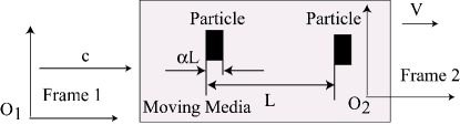
Figure 9: Relative-velocity approach to model the convection effect (Fresnel drag) in moving media. In the moving media (frame 2) the mean length between particles is $L$ and the average length of each particle is $\alpha L$.

Consider an observer $O_{2}$ in frame 2; let the nominal speed of light through a particle in the medium be $c_{m}$ when the relative velocity $V$ is zero. However, due to motion of the media, the speed of light (generated in frame 1) through particle is $c_{m}-v$ and through vacuum is $c-v$ for observer 2. The total velocity is not a linear summation of the two velocities; the effective speed of light $c_{eff,O_{2}}$ through the medium (for a fixed observer in frame $O_{2}$) is given by

$$\frac{L}{c_{eff,O_{2}}}~{}~{}=~{}\frac{\alpha L}{c_{m}-v}~{}~{}+\frac{(1-\alpha)L}{c-v}~{}~{}~{}{\mbox{i.e.,~{}~{}~{}~{}}}{c_{eff,O_{2}}}~{}=\frac{1}{\frac{\alpha}{c_{m}-v}~{}~{}+\frac{(1-\alpha)}{c-v}}.$$ (101)

The nominal speed $C_{nom}$ of the light through the media with zero relative velocity is obtained by setting $v=0$ in equation (101) as

$${c_{nom}}=\frac{1}{\frac{\alpha}{c_{m}}~{}~{}+\frac{(1-\alpha)}{c}}.$$ (102)

The effective velocity expression in equation (101) can be expanded in terms of the relative velocity $V$ as (where the higher order terms are neglected)

$$\begin{array}[]{rcl}{c_{eff,O_{2}}}&\approx&{c_{nom}}~{}+\frac{-1}{\left(\frac{\alpha}{c_{m}}~{}~{}+\frac{(1-\alpha)}{c}\right)^{2}}\left({\frac{\alpha}{c_{m}^{2}}~{}~{}+\frac{(1-\alpha)}{c^{2}}}\right)v\\ &=&{c_{nom}}~{}-\frac{c_{nom}^{2}}{c^{2}}\left({\frac{\alpha c^{2}}{c_{m}^{2}}~{}~{}+{(1-\alpha)}}\right)v\\ &=&{c_{nom}}~{}-\frac{1}{\eta^{2}}\left({\frac{\alpha c^{2}}{c_{m}^{2}}~{}~{}+{(1-\alpha)}}\right)v\end{array}$$ (103)

where $\eta$ is the media’s coefficient of refraction. If $\alpha$ is small, then the expression in equation (103) can be approximated by

$${c_{eff,O_{2}}}~{}\approx~{}~{}{c_{nom}}~{}-\frac{1}{\eta^{2}}v.$$ (104)

Rewriting in terms of observer $O_{1}$ in frame 1, by adding $v$ to the expression, leads to

$$\begin{array}[]{rcl}c_{eff,O_{1}}&=&{c_{eff,O_{2}}}+v~{}=~{}{c_{nom}}~{}-\frac{1}{\eta^{2}}v+v\\ &=&{c_{nom}}+\left(1-\frac{1}{\eta^{2}}\right)v,\end{array}$$ (105)

which is the same as Fresnel’s expression.

5 Conclusions

This article presented a Weber-type, relative-velocity-dependent electromagnetism model. It is shown that the model: (i) captures relativistic effects in optics, high-energy particles, and gravitation; and (ii) explains the apparent discrepancies in experimental energy measurements.

References

- [1] A. K. T. Assis and H. T. Silva. Comparison between weber’s electrodynamics and classical electrodynamics. Pramana — Journal of Physics, 55(3):393–404, September 2000.
- [2] J. J. Turin and H. R. Crane. The absorption of high energy electrons, Part II. Physical Review, 52:610–613, September 15 1937.
- [3] C. D. Ellis and W. A. Wooster. The average energy of disintegration of Radium E. Proceedings of the Royal Society of London. Series A, Containing Papers of a Mathematical and Physical Character, 117(776):109–123, December 1 1927.
- [4] E. Madgwick. The -ray spectrum of Ra E. Proceedings of the Cambridge Philosophical Society, 23:982–984, October 24 1927.
- [5] F. A. Scott. Energy spectrum of the beta-rays of Radium E. Physical Review, 48:391–395, September 1 1935.
- [6] P. C. Ho and M. H. Wang. Beta-ray spectrum of Radium E. Chinese Journal of Physics, 2(1):1–9, April 1936.
- [7] M. M. Slawsky and H. R. Crane. The absorption of high energy electrons, Part IV. Physical Review, 59:1203–1210, December 15 1939.
- [8] J. R. Richardson and F. N. D. Kurie. The radiations emitted from artificially produced radioactive substances. Physical Review, 50:999–1006, 1, December 1936.
- [9] L. H. Martin and A. A Townsend. The -ray spectrum of Ra E. Proceedings of the Royal Society of London. Series A, Containing Papers of a Mathematical and Physical Character, 170(941):190–205, 1, March 1939.
- [10] G. J. Neary. The -Ray Spectrum of Radium E. Proceedings of the Royal Society of London. Series A, Mathematical and Physical Sciences, 175(960):71–87, March 28 1940.
- [11] H. Goldstein. Classical Mechanics. Addison-Wesley, Menlo Park, CA, second edition, 1980.
- [12] J. J. Thomson. Cathode rays. The London, Edinburgh, and Dublin Philosophical Magazine and Journal of Science, Fifth Series, 44(269), October 1897 (reprinted in Classical Scientific Papers, Physics, by American Elsevier Publishing Company, Inc., New York, 1964, pp. 77-100).
- [13] James Bradley. A Letter from the Reverend Mr. James Bradley Savilian Professor of Astronomy at Oxford, and F.R.S. to Dr. Edmond Halley Astronom. Reg., & c. Giving an Account of a New Discovered Motion of the Fix’d. Stars. Philosophical Transactions, 35:637–661, 1727.
- [14] Kenneth Brecher. Is the speed of light independent of the velocity of the source? Physical Review Letters, 39(17):1051–1054, 24 October 1977.
- [15] Thomas R. Phipps, Jr. Relativity and aberration. American Journal of Physics, 57(6):549–551, June 1989.
- [16] Max Born. Einstein’s Theory of Relativity. Dover Publication, Inc., New York, revised edition, 1962.
- [17] A. A. Michelson and E. W. Morley. Influence of motion of the medium on the velocity of light. American Journal of Science, 31(185):377–386, May 1886.