No large-angle correlations on the non-Galactic microwave sky

Abstract

We investigate the angular two-point correlation function of temperature in the WMAP maps. Updating and extending earlier results, we confirm the lack of correlations outside the Galaxy on angular scales greater than about 60 degrees at a level that would occur in 0.025 per cent of realizations of the concordance model. This represents a dramatic increase in significance from the original observations by the COBE-DMR and a marked increase in significance from the first-year WMAP maps. Given the rest of the reported angular power spectrum $C_{\ell}$, the lack of large-angle correlations that one infers outside the plane of the Galaxy requires covariance among the $C_{\ell}$ up to $\ell=5$. Alternately, it requires both the unusually small (5 per cent of realizations) full-sky large-angle correlations, and an unusual coincidence of alignment of the Galaxy with the pattern of cosmological fluctuations (less than 2 per cent of those 5 per cent). We argue that unless there is some undiscovered systematic error in their collection or reduction, the data point towards a violation of statistical isotropy. The near-vanishing of the large-angle correlations in the cut-sky maps, together with their disagreement with results inferred from full-sky maps, remain open problems, and are very difficult to understand within the concordance model.

1 Introduction

Over a decade ago, the Cosmic Background Explorer Differential Microwave Radiometer (COBE-DMR) first reported a lack of large-angle correlations in the two-point angular-correlation function, $\mathcal{C}(\theta)$, of the cosmic microwave background (CMB) (Hinshaw et al., 1996). This was confirmed by the Wilkinson Microwave Anisotropy Probe (WMAP) team in their analysis of their first year of data (Spergel et al., 2003), and by us in the WMAP three-year data (Copi et al., 2007). Those findings have since been confirmed by Hajian (2007) and Bunn & Bourdon (2008). Here, we present a more detailed analysis of the three-year and (for the first time) of the five-year WMAP data, confirming and strengthening our previous results.

There is a common misconception that this lack of angular correlations is equivalent to the low quadrupole in the two-point angular power spectrum, which on its own does not have sufficient statistical significance to challenge the canonical paradigm. It is typically assumed both that the angular power spectrum, $C_{\ell}$, and the two point angular correlation function, $\mathcal{C}(\theta)$, contain the same information; and that consequently studying one is as good as studying both.

Actually, the exact informational equivalence between $C_{\ell}$ and $\mathcal{C}(\theta)$ holds only when the full sky is observed. Statistically they are equivalent only when the sky is statistically isotropic. But even if $C_{\ell}$ and $\mathcal{C}(\theta)$ did contain the same information, we are well aware that transforming between different representations of the same information — a time series and its Fourier transform for example — may make a real signal in the data easier or harder to detect. The Doppler peaks of the CMB, so clearly visible in the $C_{\ell}$ representation are quite invisible in the two-point correlation function.

The angular two-point function at the largest angular scales is our most direct probe of the primordial seeds of structure formation (presumably generated during cosmological inflation). We expect that the large angular scales are a direct probe of cosmological inflation, which predicts statistically isotropic CMB temperature fluctuations generated by a scale-invariant power spectrum of primordial quantum fluctuations. Without inflation, at redshift $z\simeq 1100$ observed angular scales larger than $1$ degree probe independent Hubble patches, while angular scales larger than 60 degrees probe regions that are outside of causal contact until $z\sim 1$. (More precisely, the post-inflation particle horizon subtends $\theta\mathrel{\hbox{\hbox to0.0pt{\hbox{\lower 4.0pt\hbox{$\sim$}}\hss}\hbox{$>$}}}60\degr$ at $z\mathrel{\hbox{\hbox to0.0pt{\hbox{\lower 4.0pt\hbox{$\sim$}}\hss}\hbox{$<$}}}4$ in the standard $\Lambda$CDM model.) Therefore, the epoch of reionization and other secondary effects (at $z>{\rm few}$) cannot modify the correlation function at these scales. Any correlation on top of the primordial signal must be due to local foregrounds (some contaminant at $z<\mathrm{few}$) or instrumental systematic effects.

In this work we demonstrate that outside the region of the sky dominated by our Galaxy, both of the CMB-dominated microwave bands — V and W — as well as the Internal Linear Combinations (ILC) map synthesized from them as the best map of the CMB, possess above $60\degr$ a level of two point angular correlation higher than 99.975 percent of random realizations of the best-fit $\Lambda$CDM model. Indeed, above $60\degr$, $\mathcal{C}(\theta)$ is almost entirely due to correlations involving points inside the Galaxy.

This level of statistical unlikelihood ($\mathcal{O}(10^{-4})$) should be contrasted with what could be inferred from COBE ($\mathcal{O}(10^{-2})$). This is a strong argument against the criticism that its identification as an anomaly is a posteriori. It may have been a posteriori for COBE, but its reidentification in WMAP at dramatically increased statistical significance is precisely how one goes about confirming that anomalies are actually present rather than statistical accidents of an observation.

While the full-sky map $\mathcal{C}(\theta)$ itself has unexpectedly low large-angle correlations (occurring only in 5 per cent of random realizations of the concordance model), we find that what little correlation it does have is effectively “hidden” behind the Galaxy. In fact, we find that a random rotation of the Galactic cut is as successful in masking the power only 2 per cent of the time, in agreement with the previous claim that the little correlation above $60\degr$ stems solely from two specific regions within the Galactic cut covering just 9 per cent of the sky (Hajian, 2007). This further underlies the striking lack of power outside the Galactic cut, and calls into question cosmological uses of full-sky maps even for large angular scale studies.

Finally, we demonstrate that the absence of large-angle correlations is emphatically not a matter just of the low quadrupole. Rather, given the other measured multipoles, obtaining this little large-angle correlation for the cut sky maps (i.e. the part outside the Galaxy) requires carefully tuning $C_{2}$, $C_{3}$, $C_{4}$, and $C_{5}$. There is also a strong indication that it is not enough to find a model in which the theoretical $C_{\ell}$ yield a very small correlation function on large angular scales. This is because, even if the theoretical $C_{\ell}$ were to be set equal to those that are inferred from the cut-sky $\mathcal{C}(\theta)$ — so that the expected $\mathcal{C}(\theta)$ nearly vanished above $60\degr$ — an actual realization of Gaussian-random statistically independent $a_{\ell m}$ with these ${C}_{\ell}$ would yield different observed $\mathcal{C}_{\ell}$ because of cosmic variance. $C(\theta>60\degr)$ would then not be nearly so close to zero. Thus getting $C(\theta>60\degr)$ to vanish as it does seems to require covariance among the low-$\ell$ $C_{\ell}$, and thus among $a_{\ell m}$ of different $\ell$. This is in contradiction to the predictions of standard inflationary cosmological theory.

One is therefore placed between a rock and a hard place. If the WMAP ILC is a reliable reconstruction of the full-sky CMB, then there is overwhelming evidence (de Oliveira-Costa et al. (2004); Eriksen et al. (2004); Copi et al. (2004); Schwarz et al. (2004); Copi et al. (2006, 2007); Land & Magueijo (2005a, b, c, d); Rakić & Schwarz (2007); for a review see Huterer (2006)) of extremely unlikely phase alignments between (at least) the quadrupole and octopole and between these multipoles and the geometry of the Solar System — a violation of statistical isotropy that happens by random chance in far less than 0.025 per cent of random realizations of the standard cosmology. If, on the other hand, the part of the ILC (and band maps) inside the Galaxy are unreliable as measurements of the true CMB, then the alignment of low-$\ell$ multipoles cannot be readily tested, but the magnitude of the two-point angular correlation function on large angular scales outside the Galaxy is smaller than would be seen in all but a few of every 10,000 realizations.

We can only conclude that (i) we don’t live in a standard $\Lambda$CDM Universe with a standard inflationary early history; (ii) we live in an extremely anomalous realization of that cosmology; (iii) there is a major error in the observations of both COBE and WMAP; or (iv) there is a major error in the reduction to maps performed by both COBE and WMAP. Whichever of these is correct, inferences from the large-angle data about precise values of the parameters of the standard cosmological model should be regarded with particular skepticism.

Finally we note that there is no single test for statistical anisotropy. There are countless ways of breaking statistical isotropy, that is, of having $\langle a^{*}_{\ell m}a_{\ell^{\prime}m^{\prime}}\rangle\neq\mathcal{C}_{\ell}\delta_{\ell\ell^{\prime}}\delta_{mm^{\prime}}$. Any one of them can be tested against the data but no single test can cover all possibilities. Different tests will be sensitive to different ways of breaking statistical isotropy. Thus it is both a boon and a bane that there are multiple tests with varying results (e.g. non-detections of violation of statistical isotropy in Hajian_Souradeep_2006 and Dennis_Land) discussed in the literature. Ideally these tests will lead to an understanding of how statistical isotropy can be broken and may ultimately provide an explanation of the source of the signatures seen in some tests and not in others. In the remainder of this paper we provide detailed discussion of the tests we apply and the evidence and reasoning for the statements made in the previous paragraph.

2 Angular correlation function: preliminaries

The two-point correlation function of the observed CMB temperature fluctuations

$$\mathcal{C}(\theta)\equiv\overline{T(\hat{e}_{1})T(\hat{e}_{2})}_{\theta},$$ (1)

where the over-bar represents an average over all pairs of points on the sky (or at least that portion of the sky being analyzed) that are separated by an angle $\theta$. On the one hand, we are interested in this quantity as a partial characterization of the observations. On the other hand, we regard it as an (unbiased) estimator of the ensemble average of the same quantity — where the ensemble is of realizations of the sky in a particular model cosmology.

It is commonly thought that $\mathcal{C}(\theta)$ contains the same information as the angular power spectrum,

$$C_{\ell}\equiv\frac{1}{2\ell+1}\sum_{m=-\ell}^{\ell}\left|a_{\ell m}\right|^{2}.$$ (2)

(Here $a_{\ell m}$ are the coefficients of a spherical harmonic decomposition of the temperature fluctuations on the sky.) This is because, for a full sky,

$$\mathcal{C}(\theta)=\frac{1}{4\pi}\sum_{\ell=0}^{\infty}(2\ell+1)C_{\ell}P_{\ell}(\cos\theta).$$ (3)

Again the $C_{\ell}$ are regarded as most interesting to us as unbiased estimators of the ensemble average of $\left|a_{\ell m}\right|^{2}$. Furthermore, the standard inflationary model predicts that the Universe is statistically isotropic, so that the ensemble average of pairs of $a_{\ell m}$ are independent:

$$\left\langle a^{\star}_{\ell m}a_{\ell^{\prime}m^{\prime}}\right\rangle=\mathcal{C}_{\ell}\delta_{\ell\ell^{\prime}}\delta_{mm^{\prime}}.$$ (4)

Theoretically, the $C_{\ell}$ therefore encode all of the information from the sky that has cosmological significance.

Actually, $C_{\ell}$ and $\mathcal{C}(\theta)$ only contain precisely the same information for full-sky data. Their analogues in the ensemble are informationally equivalent only if, in the ensemble, the sky is statistically isotropic. This suggests that by measuring both $\mathcal{C}(\theta)$ and $C_{\ell}$ we can probe the correctness of the assumption of statistical isotropy of the Universe. Statistical isotropy is a fundamental prediction of generic inflationary models.

More importantly, it is well known that, while a function and its Fourier transform posses exactly the same information differently organized, in different circumstances one or the other may more clearly show an interesting feature. For example, a sharp delta-function spike in a time series will merely contribute equally to all modes of the associated Fourier series. It is precisely the same with the two-point angular-correlation function and its Legendre-transform, the angular power spectrum. Thus, while our theory may suggest to us that it is easier to analyze the angular power spectrum, prudence demands that we also consider the properties of the angular correlation function, all the more so since our actual measurements are done in “angle-space” not in “$\ell$-space”.

In order to highlight these differences, we use the calligraphic symbol, $\mathcal{C}$, for objects operationally defined in “angle-space” and the symbol, $C$, for quantities in “$\ell$-space”; e.g. the Legendre transform of the two-point correlation function (1) is

$$\mathcal{C}_{\ell}\equiv 2\pi\int_{-1}^{1}P_{\ell}(\cos\theta)\mathcal{C}(\theta)\mathrm{d}(\cos\theta).$$ (5)

Note that $\mathcal{C}_{\ell}$ can be negative — in contrast to the angular power spectrum $C_{\ell}$ as defined in (2).

The angular correlation functions in this work have been calculated using SpICE (Szapudi et al., 2001) at NSIDE=512 for data maps and at NSIDE=64 for the Monte Carlo studies. The map average has been subtracted in all cases. The results are shown in Fig. 1 for four different maps — the ILC map, which covers the full sky, and KQ75 cut-sky versions of the ILC, the V-band, and the W-band. In the same figure, we have plotted the Legendre transform of the angular power spectrum (cf. equation 3) calculated using both the pseudo-$C_{\ell}$ method (essentially equation 2) applied by the WMAP team in their first-year analysis, and the maximum likelihood estimates of the angular power spectrum as used by WMAP in the third- and fifth-year analysis. Finally we have plotted the expected $C(\theta)$ for the best-fit $\Lambda$CDM, and, in blue, the one-sigma cosmic-variance band around the best fit.

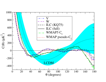
Figure 1: The two-point angular correlation function from the WMAP 5 year results. Plotted are $\mathcal{C}(\theta)$ for maps with Doppler quadrupole subtracted. The V (dashed-dotted-dotted line), W (dashed-dashed-dotted line), ILC (KQ75, dashed line) have had the KQ75 mask applied. The full-sky ILC result (solid line) is also shown. Also plotted are $C(\theta)$ from the WMAP maximum likelihood $C_{\ell}$ (dotted-dashed line), the WMAP pseudo-$C_{\ell}$ (dotted line) and the best-fit $\Lambda$CDM $C_{\ell}$. The shaded region is the one sigma cosmic variance bound on the standard $\Lambda$CDM theory.

Three striking observations should be made about $\mathcal{C}(\theta)$:

1. None of the observational angular correlation functions visually match the expectations from the theoretical model.

2. All of the cut-sky map curves are very similar to each other, and they are also very similar to the Legendre transform of the pseudo-$C_{\ell}$ estimate of the angular power spectrum. Meanwhile the full-sky ILC $\mathcal{C}(\theta)$ and the Legendre transform of the MLE of the $C_{\ell}$ agree well with each other, but not with any of the others.

3. The most striking feature of the cut-sky (and pseudo-$C_{\ell}$) $\mathcal{C}(\theta)$, is that all of them are very nearly zero above about $60\degr$, except for some anti-correlation near $180\degr$. This is also true for the full-sky curves, but less so.

In order to be more quantitative about these observations, we must adopt some statistic that measures large-angle correlations. This means that we must identify some norm that measures the difference between two functions over a range of angles. Different choices of norm, or different choices for the angular range, will give slightly different numerical results for the improbability of the above observations; however, as we shall see, the observations are so unlikely that we can be confident that reasonable choices of the norm lead to similar results.

In their analysis of the first year data, the WMAP team defined the $S_{1/2}$ statistic (Spergel et al., 2003)

$$S_{1/2}\equiv\int_{-1}^{1/2}\left[\mathcal{C}(\theta)\right]^{2}\mathrm{d}(\cos\theta).$$ (6)

While the choice of $1/2$ as the upper limit of the integral, and the particular choice of a square norm were a posteriori, they are neither optimized nor particularly special. In fact, this two-point correlator is the most basic quantity to study and $S_{1/2}$ is probably the simplest statistic that tests the total amount of correlations at large angles. Moreover, the absence of large-angle correlations was noted by the COBE team (though without definition of a particular statistical measure), and the choice of $\sim 60\degr$ is clearly suggested by the COBE-DMR4 results (Hinshaw et al., 1996).

Although the choice of $S_{1/2}$ was a posteriori for the analysis of the first year of data from WMAP, it is not for the present analysis of three and five year WMAP data. In their three and five year data releases the WMAP team has improved the calibration of the CMB maps and their understanding of systematic issues. Thus, there was the possibility that the lack of correlation would go away, but — as demonstrated below — it persists.

Table 1: The $\mathcal{C}_{\ell}$ calculated from $\mathcal{C}(\theta)$ for the various data maps. The WMAP (pseudo and reported MLE) and best-fit theory $C_{\ell}$ are included for reference in the bottom five rows.

Data	$S_{1/2}$	$P(S_{1/2})$	$6\mathcal{C}_{2}/2\pi$	$12\mathcal{C}_{3}/2\pi$	$20\mathcal{C}_{4}/2\pi$	$30\mathcal{C}_{5}/2\pi$
Source	$(\mu\mathrm{K})^{4}$	(per cent)	$(\mu\mathrm{K})^{2}$	$(\mu\mathrm{K})^{2}$	$(\mu\mathrm{K})^{2}$	$(\mu\mathrm{K})^{2}$
V3 (kp0, DQ)	$1288$	$0.04$	$77$	$410$	$762$	$1254$
W3 (kp0, DQ)	$1322$	$0.04$	$68$	$450$	$771$	$1302$
ILC3 (kp0, DQ)	$1026$	$0.017$	$128$	$442$	$762$	$1180$
ILC3 (kp0), $\mathcal{C}(>60\degr)=0$	$0$	—	$84$	$394$	$875$	$1135$
ILC3 (full, DQ)	$8413$	$4.9$	$239$	$1051$	$756$	$1588$
V5 (KQ75)	$1346$	$0.042$	$60$	$339$	$745$	$1248$
W5 (KQ75)	$1330$	$0.038$	$47$	$379$	$752$	$1287$
V5 (KQ75, DQ)	$1304$	$0.037$	$77$	$340$	$746$	$1249$
W5 (KQ75, DQ)	$1284$	$0.034$	$59$	$379$	$753$	$1289$
ILC5 (KQ75)	$1146$	$0.025$	$81$	$320$	$769$	$1156$
ILC5 (KQ75, DQ)	$1152$	$0.025$	$95$	$320$	$768$	$1158$
ILC5 (full, DQ)	$8583$	$5.1$	$253$	$1052$	$730$	$1590$
WMAP3 pseudo-$C_{\ell}$	$2093$	$0.18$	$120$	$602$	$701$	$1346$
WMAP3 MLE $C_{\ell}$	$8334$	$4.2$	$211$	$1041$	$731$	$1521$
Theory3 $C_{\ell}$	$52857$	$43$	$1250$	$1143$	$1051$	$981$
WMAP5 $C_{\ell}$	$8833$	$4.6$	$213$	$1039$	$674$	$1527$
Theory5 $C_{\ell}$	$49096$	$41$	$1207$	$1114$	$1031$	$968$

The calculation of $S_{1/2}$ by direct use of (6) is susceptible to noise in $\mathcal{C}(\theta)$. To avoid this we calculate $S_{1/2}$ directly from $\mathcal{C}_{\ell}$ as

$$S_{1/2}=\frac{1}{(4\pi)^{2}}\sum_{\ell,\ell^{\prime}}(2\ell+1)(2\ell^{\prime}+1)\mathcal{C}_{\ell}\mathcal{I}_{\ell,\ell^{\prime}}\left(1/2\right)\mathcal{C}_{\ell^{\prime}}.$$ (7)

The calculation of $\mathcal{I}_{\ell,\ell^{\prime}}(x)$ is described in Appendix A. The $\mathcal{C}_{\ell}$ smooth over $\mathcal{C}(\theta)$ as defined in Eq. (5).

We can use $S_{1/2}$ to characterize the likelihood of the observed correlation function. For the COBE-DMR data (Hinshaw et al., 1996), there are relatively large error bars on $\mathcal{C}(\theta)$, which are consistent with a wide range of $S_{1/2}$ ranging from under $1000\,\mathrm{(\mu{K})^{4}}$ to approximately $6000\,\mathrm{(\mu{K})^{4}}$. But to understand the significance of these values, we must compare them to those obtained from random realizations of the sky in the concordance $\Lambda$CDM model with the best-fit parameters. For this comparison, we generated maps based on the WMAP five-year $\Lambda$CDM MCMC parameter chain. There are 20,401 sets of parameters in this chain. We computed the $C_{\ell}$ for these parameter sets using CAMB (Lewis et al., 2000). For the $C_{\ell}$ corresponding to each set of parameters, we generated a number of random maps (i.e. maps with $a_{\ell m}$ drawn from Gaussian distributions with zero mean and variance $C_{\ell}$) based on the weight assigned to each WMAP MCMC parameter set. This produced a total of 99,997 maps at NSIDE=64. From the distribution of $S_{1/2}$ values generated we calculated the probability ($p$-value) of randomly attaining a $S_{1/2}$ as low as those we found. For COBE-DMR the maximum value of $S_{1/2}$ of $6000\,\mathrm{(\mu{K})^{4}}$ corresponds to a 3 per cent chance of obtaining this little angular correlation in a random realization of the concordance model.

3 Basic results

Table 1 lists (columns 2 and 3) the value of $S_{1/2}$ and its $p$-value among the sample of 99,997 WMAP MCMC maps for the three-year and five-year maps related to those plotted in Fig. 1. These include the three and five-year V band (V3 and V5) and W band (W3 and W5) cut-sky maps. Also the ILC map in three-year and five-year versions, both full and cut sky. We use the kp0 cut for three-year maps and the KQ75 cut in the case of the five-year maps. The five-year cut-sky maps are presented both as measured and corrected for the contribution of the Doppler quadrupole (DQ), see e.g. Schwarz et al. (2004). (All maps are corrected by the WMAP team for the Doppler dipole.)

The Legendre transform of $\mathcal{C}(\theta)$ gives us $\mathcal{C}_{\ell}$, and these values are also listed in Table 1 (columns 4–7) for $\ell=2\hbox{--}5$. Also included in the table, in the bottom five rows, are the $\ell=2\hbox{--}5$ values of the WMAP three-year pseudo-$\mathcal{C}_{\ell}$, the WMAP three-year $\mathcal{C}_{\ell}$ as extracted by the WMAP team using a maximum likelihood analysis (the reported values of the $\mathcal{C}_{\ell}$), the reported five-year values of the $\mathcal{C}_{\ell}$, and the theoretical $\mathcal{C}_{\ell}$ computed using the best-fit parameter values as reported both in the three-year and the five-year WMAP analysis. Finally and importantly, the table also shows the values of $S_{1/2}$ and their $p$-values computed from the Legendre transform of these angular power spectra.

The three cut-sky maps, V, W, and ILC, whether three-year or five-year, are all in good agreement with each other. They all have very low values of $S_{1/2}$ — almost two orders-of-magnitude below the predictions of the theory. In both the three and five-year ILC outside the Galaxy, the probability that such low values could happen by chance is extraordinarily low — only $0.025$ per cent. This low probability is entirely consistent with the original finding of COBE-DMR (Hinshaw et al., 1996) described above, however the error bars on $\mathcal{C}(\theta)$ (and hence on $S_{1/2}$) have declined substantially, with the WMAP value of $S_{1/2}$ being at the absolute lowest end of what was consistent with COBE, and with much smaller error bars. This dramatic decline in the error bars, while honing in on the very low end of the COBE-DMR range, is exactly what one would expect from the absence of large-angle correlations in the CMB sky, and not at all what one would expect if the low $S_{1/2}$ in COBE-DMR (and in WMAP) was merely a statistical fluctuation in the measurement.

We also consider the case where there is exactly zero large scale angular correlations. That is, we set $\mathcal{C}(\theta\geq 60\degr)=0$ and extract the $\mathcal{C}_{\ell}$ as a Legendre transform for the ILC (kp0) map. This “theory” produces low-$\ell$ $\mathcal{C}_{\ell}$ of approximately the same value as for the $\mathcal{C}(\theta)$ from the cut-sky maps. On the one hand this is consistent with the statement that there is little correlation on large angular scales and thus the $\mathcal{C}_{\ell}$ for low-$\ell$ are dominated by small angular scales. On the other hand, this shows that the data is consistent with there being no correlations on large angular scales.

We note that it is difficult to enforce $\mathcal{C}(\theta)=0$ in the context of a statistically isotropic model. Even if a model were found that predicted the observed $C_{\ell}$ as the expected means of the $\left|a_{\ell m}\right|^{2}$ (as in equation 4), any actual realization of the Universe would produce $C_{\ell}$ that were substantially different. Indeed, we have found that $>97$ per cent of realizations of such a Universe would have values of $S_{1/2}$ greater than the observed value (see section 5.1).

The results from the full-sky ILC map, also show low values of $S_{1/2}$; however, with less remarkable $p$-values of 5 per cent in contrast to $0.02\hbox{--}0.04$ per cent for the various cut-sky maps. Similarly, the full sky ILC maps have larger quadrupoles than the cut-sky maps (though still lower than expected from theory), and octopoles consistent with theory. These full-sky maps are in good agreement with the WMAP-reported MLE $C_{\ell}$. Meanwhile the pseudo-$C_{\ell}$ based on the kp2 sky-cut (which cuts less of the sky than the kp0 cut) are intermediate between the kp0 cut-sky map results and the full-sky results.

Thus the full-sky results seem inconsistent with cut-sky results and they appear inconsistent in a manner that implies that most of the large-angle correlations in reconstructed sky maps are inside the part of the sky that is contaminated by the Galaxy.

4 Missing power or unfortunate alignment?

An important question to consider is whether the extremely low large-angle correlations in the cut-sky WMAP maps are a general result of cutting the maps or is specific to the orientation of the cut. That is, should we expect a loss of large-angle correlations in a cut-sky map or is the alignment of the cut with the Galaxy important. To address this question the full-sky five-year ILC map was randomly rotated (that is, set its north pole in a random direction and draw its azimuthal angle from a uniform distribution) 300,000 times. For each random rotation we masked the map with the Galactic KQ75 mask, which is now, therefore, randomly oriented relative to the original map and re-computed the quadrupole, octopole and $S_{1/2}$ statistic.

The analysis shows that the true cut-sky quadrupole and octopole are not terribly unusual compared to those inferred from the rotated-then-cut (RTC) maps. In 7.6 per cent of these RTC maps the quadrupole is smaller than that of the ILC with the originally placed cut, while 2.5 per cent have a smaller octopole. Therefore, if we looked at the quadrupole and octopole alone we would conclude that an arbitrarily oriented mask is only moderately unlikely to produce low-$\ell$ power in the cut-sky ILC. Conversely, the particular alignment of the Galaxy with the part of the sky on which the low-$\ell$ power is concentrated is only moderately important.

On the other hand, in the RTC maps $S_{1/2}=11900\,\mathrm{(\mu K)^{4}}$ with variance $7300\,\mathrm{(\mu K)^{4}}$, a very high value relative to the original cut ILC map ($1152\,\mathrm{(\mu K)^{4}}$, see Table 1). Only 2 per cent of these rotated maps have $S_{1/2}$ lower than the ILC with the original cut. (Recall that $S_{1/2}\simeq 8583\,\mathrm{(\mu K)^{4}}$ for the full-sky ILC is already low, with a $p$-value of only about 5 per cent.) Thus it is quite unlikely for an arbitrary cut to suppress the large-angle correlations to the extent observed in the cut-sky ILC map. Conversely, it is quite likely that the observed absence of large-angle correlations outside the KQ75 cut is due to the alignment of the Galaxy with the regions on the sky where such correlations are maximized. This result is in good agreement with the result from Hajian (2007) that the little correlation above $60\degr$ stems from two specific regions within the Galactic cut covering just 9 per cent of the sky.

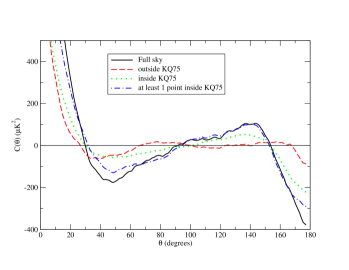
Figure 2: The two-point angular correlation function from the WMAP 5 year results. Plotted are $\mathcal{C}(\theta)$ for the ILC calculated separately the part of the sky outside the KQ75 cut (dashed line), inside the KQ75 cut (dotted line), and on the part of the sky with at least on point inside the KQ75 cut (dotted-dashed line). For better comparison to the full-sky $\mathcal{C}(\theta)$ (solid line), the partial-sky $\mathcal{C}(\theta)$ have been scaled by the fraction of the sky over which they are calculated.

It appears that our microwave background sky has anomalously low angular correlations everywhere outside the Galactic mask, but not within. In Fig. 2 we plot $\mathcal{C}(\theta)$ for the WMAP 5 year ILC map calculated separately on the part of the sky outside the KQ75 cut, inside the KQ75 cut, and on the part of the sky with at least one point inside the KQ75 cut. For better comparison to the full-sky $\mathcal{C}(\theta)$ (also plotted), the partial-sky $\mathcal{C}(\theta)$ have been scaled by the fraction of the sky over which they are calculated. This shows that the full-sky $\mathcal{C}(\theta)$ is very close to $\mathcal{C}(\theta)$ calculated from the masked region. Meanwhile $\mathcal{C}(\theta)$ calculated outside the Galactic mask is similar to neither, and much closer to zero in magnitude.

Figure 2 shows two other interesting peculiarities of the measured angular correlation function. First, the full-sky $\mathcal{C}(\theta)$ is particularly closely mimicked by the $\mathcal{C}(\theta)$ computed so that at least one of the points is inside the masked region; the agreement between the two at large angles (above approximately $60\degr$) is nearly perfect. Moreover, all four correlation functions shown in the figure vanish at nearly the same angle, $\theta\sim 90\degr$. While at this time we do not understand the origin or significance of these two effects, we wish to point them out because it is possible that they will be useful for successful theoretical or systematic explanations of the vanishing correlation function.

The evidence we present strongly suggests that the full-sky ILC map does not represent a statistically isotropic microwave sky. If the region outside the cut is a reliable representation of the CMB then we should focus on the angular correlation for cut skies. As shown above this leads to a $p$-value of 0.025 per cent for the standard $\Lambda$CDM model (see Table 1). Furthermore, the WMAP reported MLE $\mathcal{C}_{\ell}$, which assumes Gaussianity and statistical isotropy in their calculation, are in good agreement with the full-sky $\mathcal{C}_{\ell}$ and $\mathcal{C}(\theta)$, but not with their cut-sky equivalents, whereas, the cut-sky $\mathcal{C}_{\ell}$ and $\mathcal{C}(\theta)$ are in good agreement with the pseudo-$C_{\ell}$ (see Table 1 and figure 1). This casts doubt on the validity of the reported low-$\ell$ $C_{\ell}$.

5 So, is the large scale CMB anomalous or not?

It has been suggested that there is nothing particularly anomalous about the large-angle CMB (Efstathiou, 2004; Gaztanaga et al., 2003; Slosar et al., 2004). The argument goes something like this: (a) the two-point angular correlation function $\mathcal{C}(\theta)$ and the angular power spectrum $C_{\ell}$ contain the same information; (b) not only does theory tell us that the $C_{\ell}$ are the “relevant” variables, but, since they are discrete and finite in number, we can apply standard statistical techniques to compare observations with theoretical predictions; when we do so, we find that only $C_{2}$ is far below the expected value, but still at a level that happens by chance 10 per cent of the time in the concordance model.

We have already pointed out above that (a) contains two fallacies. First, $\mathcal{C}(\theta)$ and $C_{\ell}$ are equivalent only on a full sky. Second, formal equivalence is not the only question, signals are often more visible in one representation of the data than in a different, though formally equivalent one. If this were not so, then there would be no need for Fourier analysis. Nor would we need to perform great music — we could simply read the score.

Point (b) is correct if the Inflationary Cold Dark Matter ($\Lambda$CDM) cosmological model is true. This model tells us that the spherical harmonic coefficients $a_{\ell m}$ are independent Gaussian random variables, and that the sky is statistically isotropic, so that the off-diagonal covariances of the estimator $C_{\ell}$ (as defined in Eq. 2) vanishes in linear theory. This vastly simplifies statistical analysis of the CMB in the context of $\Lambda$CDM. However, in advancing the case for a particular cosmological model we are required not just to determine the best-fit parameters of the model but to test the assumptions and other predictions of the model. This includes the prediction of statistical isotropy, and consequently that the $a_{\ell m}$ are independent of one another.

There is already considerable evidence that if one analyzes the full-sky ILC map that one finds difficult-to-explain deviations from statistical isotropy, such as the alignment of the octopole and quadrupole with each other and with the geometry of the Solar System (for example de Oliveira-Costa et al. (2004); Eriksen et al. (2004); Schwarz et al. (2004); Land & Magueijo (2005a)). These analyses require full-sky data for any statistical power, and so, in particular, might be explained by Galactic foreground contamination (though it would be an odd coincidence for Galactic contamination to cause alignment with the Solar System). The calculation of $\mathcal{C}(\theta)$, as we have seen, can be done on a cut sky.

5.1 Are just the low-$\ell$ $C_{\ell}$ incorrect?

Perhaps the standard assumptions of statistical isotropy and Gaussianity are correct and only the low-$\ell$ $C_{\ell}$ are incorrectly predicted by the standard model. If this were the case then the $a_{\ell m}$ could still be Gaussian random variables and some new physics would be needed to explain the low-$\ell$ $C_{\ell}$, e.g., by giving up the scale invariance of the primordial power spectrum, which could be caused by a feature in the inflationary potential.

To study this possibility we replaced $C_{2}$ through $C_{20}$ in the best fit $\Lambda$CDM model with the values extracted from the cut-sky ILC five-year map. From these $C_{\ell}$ 200,000 random maps were created, masked, and $S_{1/2}$ computed. Under the assumptions of Gaussianity and statistical isotropy of these $C_{\ell}$ only 3 per cent of the generated maps had $S_{1/2}$ less than $1152\,\mathrm{(\mu K)^{4}}$ (the cut-sky ILC5 value from Table 1). Thus even if the $C_{\ell}$ are set to the specific values that produce such a low $S_{1/2}$ a Gaussian random, statistically isotropic realization is 97 per cent unlikely to produce the observed sky. Again this shows that either (i) the low-$\ell$ $C_{\ell}$ are correlated, thus breaking statistical isotropy, or (ii) our Universe is a 97 per cent unlikely realization of an alternative model that deviates from the standard one as required to produce the low-$\ell$ $C_{\ell}$.

5.2 Statistics of $C(\theta)$

Once we have decided to calculate $\mathcal{C}(\theta)$, we are forced to ask how best to analyze it statistically. One option would be to compare the $\mathcal{C}(\theta)$ inferred from a particular map to the $C(\theta)$ one expects from theory. Thus one would define

$$C^{\mathrm{th}}(\theta)\equiv\frac{1}{4\pi}\sum_{\ell=0}^{\infty}(2\ell+1)C_{\ell}^{\mathrm{th}}P_{\ell}(\cos\theta),$$ (8)

for a particular set of parameters (say the best-fit values) of the concordance model. This is what is plotted in figure 1 as the $C(\theta)$ of the best-fit $\Lambda$CDM model.

One would next define some functional norm and compute

$$N^{\mathrm{obs-\Lambda{CDM}}}\equiv||\mathcal{C}(\theta)-C^{\mathrm{th}}(\theta)||$$ (9)

where we imply a suitable average over a range of $\theta$ on the right-hand side. This norm could serve as a statistic to compare the two-point correlation function inferred from the data, or some subset of the data to the theory. The shaded band around $C^{\mathrm{th}}(\theta)$ in figure 1 (cosmic variance) reflects this notion that one somehow expects the inferred $\mathcal{C}(\theta)$ to lie inside this band.

The statistic originally suggested by the WMAP team for comparing observations of large-angle correlations to theory, $S_{1/2}$, does not fall into the above class of statistics. This is because it captures that what is strange about the inferred angular correlation function $\mathcal{C}(\theta)$ is not that it is different than theory for $\theta\ga 60\degr$, but rather that it is so close to zero. Thus $S_{1/2}$ is designed to test an alternative simple hypothesis — that there are no correlations above $60\degr$. In the language of equation (9) $S_{1/2}$ is in the class of statistics

$$N^{\mathrm{obs-zero}}\equiv||\mathcal{C}(\theta)-0||.$$ (10)

There is another lesson to be learned from the preceding results. Cosmological inflation predicts that there are fluctuations on all scales, whereas many alternative models of structure formation, like cosmic defects, would predict the absence of fluctuations on super-horizon scales. By looking at scales above $1$ degree on the sky the inflationary prediction is tested at the time of photon decoupling, and by looking at the largest angular scales, we can test it in the more recent Universe since the physical Hubble scale $r_{H}(z)=1/H(z)$ is observed at the angle $\theta=r_{H}(z)/d_{\rm a}(z)$ and angular distance $d_{\rm a}(z)=[1/(1+z)]\int_{0}^{z}[1/H(z^{\prime})]\mathrm{d}z^{\prime}$. For the best-fit parameters of the concordance model, the lack of correlations at larger $60$ degrees means, that scales that crossed into the Hubble radius below a redshift $\approx 1.5$ are uncorrelated.

Instead of $S_{1/2}$, Hajian (2007) advocates the use of a covariance-weighted integral over $\mathcal{C}(\theta)$,

$$A(x)\equiv\int_{-1}^{x}\mathrm{d}(\cos\theta)\int_{-1}^{x}\mathrm{d}(\cos\theta^{\prime})\mathcal{C}(\theta)F^{-1}(\theta,\theta^{\prime})\mathcal{C}(\theta^{\prime}),$$ (11)

where

$$F(\theta,\theta^{\prime})\equiv\left<(C(\theta)-\langle C(\theta)\rangle)(C(\theta^{\prime})-\langle C(\theta^{\prime})\rangle)\right>,$$ (12)

and $\left<\cdots\right>$ represents an ensemble average, i.e. an average over realizations of the underlying $\Lambda$CDM model. As Hajian notes, $A(1/2)=S_{1/2}$ in the limit of uncorrelated $\mathcal{C}(\theta)$. However, just because $C(\theta)$ and $C(\theta^{\prime})$ are correlated in the standard theory does not make $A(1/2)$ a more correct statistic than $S_{1/2}$. For tests against the standard theory the $A(x)$ statistic provides another statistic; one that accounts for the theory correlations. However, as discussed above, it has repeatedly been shown that there are correlations among the low-$\ell$ multipole moments (and multipole vectors) of the full sky that are not consistent with the standard theory. In this case it is not possible to compute $F(\theta,\theta^{\prime})$ because the ensemble over which to average is unknown. Therefore, while it is somewhat reassuring that by using $A(x)$ Hajian (2007) confirms our earlier result (Copi et al., 2007) showing $\mathcal{C}(\theta)$ for cut skies violates the fundamental model assumption of statistical isotropy, it is not clear that any strong inference should be drawn from differences in statistical significance between results for $A(1/2)$ and $S_{1/2}$.

Table 2: $S_{1/2}$ (in $(\mu\mathrm{K})^{4}$) obtained by minimizing with respect to $C_{\ell}$. We show the statistic for the best-fit theory and WMAP, as a function of the cutoff multipole $\ell_{\mathrm{max,tune}}$ (the minimization has been performed by varying all $\ell$ in the range $2\leq\ell\leq\ell_{\mathrm{max,tune}}$ and fixing $\ell>\ell_{\mathrm{max,tune}}$). Also shown is the 95 per cent confidence region of the minimized $S_{1/2}$ derived from chain 1 of the WMAP MCMC parameter fit. In the bottom row, we remind the reader that the measured value of $S_{1/2}$ outside the cut is $1152\,\mathrm{(\mu K)^{4}}$ (see Table 1 for more details).

$C_{\ell}$	Maximum tuned multipole, $\ell_{\mathrm{max,tune}}$
Source	$2$	$3$	$4$	$5$	$6$	$7$	$8$
Theory	$7624$	$922$	$118$	$23$	$7$	$3$	$0.7$
Theory 95 per cent	$6100$–$12300$	$750$–$1500$	$100$–$200$	$20$–$40$	$7$–$14$	$3$–$6$	$1$–$3$
WMAP	$8290$	$2530$	$2280$	$800$	$350$	$150$	$130$
ILC5 (KQ75)	$1152$

The $A(x)$ statistic suggested by Hajian (2007) and the MLE estimator for the $C_{\ell}$ are examples of optimal statistics. These statistics have minimum variance for a specific theory. In both these cases the assumptions of Gaussianity and statistical isotropy are employed. Once a theory is established these statistics make optimal use of the available data to extract the most precise possible values of model parameters or of values of summary properties of the data, for example of the $C_{\ell}$. However, when testing the validity of a theory they only provide another statistic and may not provide the best test of the assumptions of that theory. In the work presented here, we implicitly assume a flat weighting of the pixel temperatures in computing $\mathcal{C}(\theta)$; see Eq. (1). Furthermore, when assessing the lowness of $\mathcal{C}(\theta)$ at large scales, we do not rely on any particular underlying theory and assume a flat weighting implicit in the definition of our statistic $S_{1/2}$. We find that if we assume Gaussianity and statistical isotropy (through use of the MLE $C_{\ell}$, see Table 1) then the standard model has a $p$-value of 5 per cent. However, if we do not make these assumptions then the standard model only has a $p$-value of 0.025 per cent. Without a much more detailed analysis, it seems to us that a flat weighting is more robust against incorrect assumptions about the actual statistical distribution than an optimal weighting. In order to definitively answer that question one would need to analyze the higher ($n$-point) correlation functions at large angular scales, which is beyond the scope of this work.

Finally, we again emphasize that what is anomalous about the observed large-angle correlations is not how poorly they match the theory, but rather how well they agree with the very simple alternative phenomenological hypothesis that there are no large-angle correlations — $\mathcal{C}(\theta>60\degr)=0$. The construction of $N^{\mathrm{obs-\Lambda{CDM}}}$, might indeed benefit from an attempt to remove expected correlations through $F(\theta,\theta^{\prime})$, as in Hajian (2007); however, the theoretical model against which $N^{\mathrm{obs-zero}}$ compares the observations has $F(\theta,\theta^{\prime})\equiv 0$ for the relevant $\theta$.

5.3 Minimizing $S_{1/2}$

Once we have understood that what is anomalous about $\mathcal{C}(\theta)$ is how close it is to zero, we can understand that what is strange about the low-$\ell$ $C_{\ell}$ is not just how low $C_{2}$ is, but also how the various $C_{\ell}$ are correlated with each other.

We now probe the sensitivity of $S_{1/2}$ to ranges of $\ell$. Given that small angles can affect low-$\ell$ results, it is also the case that higher $\ell$ can affect the larger angles. One way to see this is to determine how the $C_{\ell}$ for low-$\ell$ must be adjusted to attain a low $S_{1/2}$. This is not done by setting some range of $C_{\ell}$ to zero. Instead, given a set of $C_{\ell}$ for $\ell>\ell_{\mathrm{max,tune}}$ we can find the values of $C_{\ell}$ for $2\leq\ell\leq\ell_{\mathrm{max,tune}}$ that minimize $S_{1/2}$  by regarding $S_{1/2}$ as a function of $C_{\ell}$ using equations (3) and (6).

We consider two sets of $C_{\ell}$, the first from the $\Lambda$CDM theory, the second as reported by WMAP. Table 2 shows the minimum $S_{1/2}$ we find for each value of $\ell_{\mathrm{max,tune}}$. In the table, we provide the values for the best-fit $\Lambda$CDM model and the reported WMAP $C_{\ell}$. We also provide the 95 per cent confidence ranges based on the WMAP MCMC parameter set chain where the minimum $S_{1/2}$ was calculated independently for each model.

To attain $S_{1/2}\leq 1152\,\mathrm{(\mu{K})^{4}}$ (the value found in the masked ILC map, see Table 1) from the best-fit theory requires tuning both $C_{2}$ and $C_{3}$. Thus even the theory requires more fine-tuning than just the quadrupole to be low in order to be consistent with observations. The minimum in Table 1 was attained for $6C_{2}/2\pi=149\,\mathrm{(\mu{K})^{2}}$ and $12C_{3}/2\pi=473\,\mathrm{(\mu{K})^{2}}$. In general for the theory we need to tune at least up to $\ell_{\mathrm{max,tune}}=3$ and can almost always find a low $S_{1/2}$ if we tune up to $\ell_{\mathrm{max,tune}}=4$.

For the WMAP $C_{\ell}$ even more tuning is required. Note that the WMAP $C_{2}$ is already approximately tuned to produce the minimum $S_{1/2}$ given the rest of the $C_{\ell}$ for $\ell>2$ (that is, from Table 1 we note that $8583\,\mathrm{(\mu{K})^{4}}\approx 8290\,\mathrm{(\mu{K})^{4}}$). To attain the low $S_{1/2}$ to match the cut-sky ILC requires tuning of values of $C_{\ell}$ up to $\ell_{\mathrm{max,tune}}=5$.

Table 2 further shows that the minimum $S_{1/2}$, that can be achieved by optimizing the low-$\ell$ $C_{\ell}$ fall off much more slowly in the WMAP $C_{\ell}$ than in the theory. By $\ell_{\mathrm{max,tune}}=8$ the minimum WMAP $S_{1/2}$ is two orders of magnitude larger than can be attained from the theory. This strongly suggests that important correlations exist in the data for $\ell\geq 8$ that do not exist in the theory. These correlations cannot be canceled by tuning the lower $\ell$ behavior.

Therefore, we conclude that a given behavior of $C(\theta)$ on large scales is not in unique relation to a behavior of $C_{\ell}$ at low-$\ell$. The former quantity receives significant contributions from $C_{\ell}$ at high $\ell$ as well; the converse is also true. Given the extremely puzzling near-vanishing power in $\mathcal{C}(\theta>60\degr)$, and given that the quadrupole and octopole are not unusually low (as shown in e.g. O’Dwyer et al. (2004)), we argue that any theoretical or observational explanation of the “low power at large scales” should concentrate on the quantity $\mathcal{C}(\theta)$.

6 Conclusions

In this paper we have studied the angular correlation function in WMAP three- and five-year maps. We have clarified the relation between various definitions of the angular correlation function, and revisited our previous calculation from Copi et al. (2007) in more detail. We confirmed that power on large angular scales — greater than about 60 degrees — is anomalously low, at 99.975 per cent CL (see Table 1). The measured angular correlation function thus disagrees with the $\Lambda$CDM theory, but, more significantly, it is consistent with a simple phenomenological “theory” — $\mathcal{C}(\theta\geq 60\degr)\equiv 0$. The significance of this disagreement (as measured by the probability of the value of $S_{1/2}$) has now increased by a factor of over 100 since it was first observed in the COBE-DMR four-year analysis.

We have shown that the cut-sky and full-sky large-scale angular correlations differ (see Table 1 and Figure 1), though the source of these discrepancies remains unknown. This shows that either the Universe is not statistically isotropic on large angular scales or that correlations are introduced in reconstructing the full sky from the observations. We have shown that even given the unusually small full-sky angular correlations (95 per cent unlikely) an unusual alignment of the Galaxy with the CMB (2 per cent of realizations) is required to explain the lack of correlations outside the Galactic region. We have further shown that simply adjusting the theoretical values of the $C_{\ell}$ does not solve the problem if the sky is representative of a Gaussian random statistically isotropic process – the cosmic variance in the $C_{\ell}$ is such that less than 3 per cent of all realizations would preserve a low value of $S_{1/2}$ .

From these results we argue that $\mathcal{C}(\theta)$ is an important quantity to study along with the usual angular power spectrum, $C_{\ell}$. The typical “rule-of-thumb” that low-$\ell$ describes large angular scales is not accurate. Any theoretical explanations for the “missing large-scale power” should concentrate on explaining the low $\mathcal{C}(\theta)$, rather than the smallness of the quadrupole and octopole, which are not nearly as significant (O’Dwyer et al., 2004). As has been pointed out by Gordon:2005ai, Rakić & Schwarz (2007) and Bunn & Bourdon (2008), any possible explanation of the multipole alignments that relies on an additive, statistically independent contribution to the microwave sky on top of the primordial one, increases the significance of the lack of angular correlation.

The CMB, as measured by WMAP in particular, provides much support for our current model of the Universe. It also points the way toward new puzzles that may affect fundamental physics. On the largest angular scales the microwave sky is inconsistent with theoretical expectations. These discrepancies between observations and theory remains an open problem. In the future, combining the current data with new information, such as new data from WMAP, observations from the Planck experiment, and polarization information (Dvorkin et al., 2008) may be key to determining the nature of the large-scale anomalies.

Appendix A Integrating products of Legendre polynomials

We wish to calculate

$$\mathcal{I}_{m,n}(x)\equiv\int_{-1}^{x}P_{m}(x^{\prime})P_{n}(x^{\prime})\mathrm{d}x^{\prime}.$$ (13)

For the special case of $x=1$ this is just the normalization

$$\mathcal{I}_{m,n}(1)=\frac{2}{2n+1}\delta_{m,n}.$$ (14)

For a general $x$ we consider two cases. When $m\neq n$ Legendre’s equation

$$(1-x^{2})P_{n}^{\prime\prime}(x)-2xP_{n}^{\prime}(x)+n(n+1)P_{n}(x)=0$$ (15)

allows us to write

$$P_{m}(x)P_{n}(x) = \frac{\mathrm{d}}{\mathrm{d}x}\left[(1-x^{2})(P_{m}^{\prime}P_{n}-P_{n}^{\prime}P_{m})\right]$$ (16)

$${}\bigm{/}[n(n+1)-m(m-1)].$$

Then using the relation

$$(1-x^{2})P_{n}^{\prime}(x)=nP_{n-1}(x)-nxP_{n}(x)$$ (17)

we find

$$\mathcal{I}_{m,n} = \bigl{\{}mP_{n}(x)\left[P_{m-1}(x)-xP_{m}(x)\right]$$ (18)

$$\quad{}-nP_{m}(x)\left[P_{n-1}(x)-xP_{n}(x)\right]\bigr{\}}$$

$${}\Bigm{/}\bigl{\{}n(n+1)-m(m+1)\bigr{\}}\quad\mbox{[for $m\neq n$]}.$$

When $m=n$ we integrate (13) by parts to get off diagonal terms (18) and use the indefinite integral

$$\int P_{n}(x)\mathrm{d}x=\frac{1}{2n+1}\left[P_{n+1}(x)-P_{n-1}(x)\right]$$ (19)

to derive the recursion relation

$$\mathcal{I}_{n,n}(x) = \bigl{\{}\left[P_{n+1}(x)-P_{n-1}(x)\right]\left[P_{n}(x)-P_{n-2}(x)\right]$$ (20)

$$\quad{}-(2n-1)\mathcal{I}_{n+1,n-1}(x)+(2n+1)\mathcal{I}_{n,n-2}(x)$$

$$\quad{}+(2n-1)\mathcal{I}_{n-1,n-1}(x)\bigr{\}}\Bigm{/}\bigl{\{}2n+1\bigr{\}}.$$

Starting from $\mathcal{I}_{0,0}(x)=x+1$ and $\mathcal{I}_{1,1}(x)=(x^{3}+1)/3$ we can calculate all the diagonal terms recursively.

With these two relations (18 and 20) we can compute and tabulate all required values of $\mathcal{I}_{m,n}$ for any $x$.

References

- Bunn & Bourdon (2008) Bunn E. F., Bourdon A., 2008, ArXiv e-prints, 0808.0341
- Copi et al. (2006) Copi C. J., Huterer D., Schwarz D. J., Starkman G. D., 2006, Mon. Not. Roy. Astron. Soc., 367, 79
- Copi et al. (2007) Copi C. J., Huterer D., Schwarz D. J., Starkman G. D., 2007, Phys. Rev. D, 75, 023507
- Copi et al. (2004) Copi C. J., Huterer D., Starkman G. D., 2004, Phys. Rev., D70, 043515
- de Oliveira-Costa et al. (2004) de Oliveira-Costa A., Tegmark M., Zaldarriaga M., Hamilton A., 2004, Phys. Rev., D69, 063516
- Dvorkin et al. (2008) Dvorkin C., Peiris H. V., Hu W., 2008, Phys. Rev., D77, 063008
- Efstathiou (2004) Efstathiou G., 2004, MNRAS, 348, 885
- Eriksen et al. (2004) Eriksen H. K., Hansen F. K., Banday A. J., Górski K. M., Lilje P. B., 2004, ApJ, 605, 14
- Górski et al. (2005) Górski K. M., Hivon E., Banday A. J., Wandelt B. D., Hansen F. K., Reinecke M., Bartelmann M., 2005, ApJ, 622, 759
- Gaztanaga et al. (2003) Gaztanaga E., Wagg J., Multamaki T., Montana A., Hughes D. H., 2003, Mon. Not. Roy. Astron. Soc., 346, 47
- Hajian (2007) Hajian A., 2007, ArXiv Astrophysics e-prints, astro-ph/0702723
- Hinshaw et al. (1996) Hinshaw G., Branday A. J., Bennett C. L., Gorski K. M., Kogut A., Lineweaver C. H., Smoot G. F., Wright E. L., 1996, ApJL, 464, L25+
- Huterer (2006) Huterer D., 2006, New Astron. Rev., 50, 868
- Land & Magueijo (2005a) Land K., Magueijo J., 2005a, Phys. Rev. Lett., 95, 071301
- Land & Magueijo (2005b) Land K., Magueijo J., 2005b, MNRAS, 357, 994
- Land & Magueijo (2005c) Land K., Magueijo J., 2005c, MNRAS, 362, L16
- Land & Magueijo (2005d) Land K., Magueijo J., 2005d, MNRAS, 362, 838
- Lewis et al. (2000) Lewis A., Challinor A., Lasenby A., 2000, ApJ, 538, 473
- O’Dwyer et al. (2004) O’Dwyer I. J., et al., 2004, ApJ, 617, L99
- Rakić & Schwarz (2007) Rakić A., Schwarz D. J., 2007, Phys. Rev., D75, 103002
- Schwarz et al. (2004) Schwarz D. J., Starkman G. D., Huterer D., Copi C. J., 2004, Phys. Rev. Lett., 93, 221301
- Slosar et al. (2004) Slosar A., Seljak U., Makarov A., 2004, Phys. Rev., D69, 123003
- Spergel et al. (2003) Spergel D. N., et al., 2003, ApJS, 148, 175
- Szapudi et al. (2001) Szapudi I., Prunet S., Colombi S., 2001, ApJL, 561, L11