Forward Correction and Fountain Codes in Delay Tolerant Networks

Abstract

Delay tolerant Ad-hoc Networks leverage the mobility of relay nodes to compensate for lack of permanent connectivity and thus enable communication between nodes that are out of range of each other. To decrease delivery delay, the information to be delivered is replicated in the network. Our objective in this paper is to study a class of replication mechanisms that include coding in order to improve the probability of successful delivery within a given time limit. We propose an analytical approach that allows to quantify tradeoffs between resources and performance measures (energy and delay). We study the effect of coding on the performance of the network while optimizing parameters that govern routing. Our results, based on fluid approximations, are compared to simulations which validate the model..

I Introduction

Delay tolerant Ad-hoc Networks make use of nodes’ mobility to compensate for lack of instantaneous connectivity. Information sent by a source to a disconnected destination can be forwarded and relayed by other mobile nodes. There has been a growing interest in such networks as they have the potential of providing many popular distributed services [1, 2, 3].

A naive approach to forward a file to the destination is by epidemic routing in which any mobile that has the message keeps on relaying it to any other mobile that falls within its radio range. This would minimize the delivery delay at the cost of inefficient use of network resources (e.g. in terms of the energy used for flooding the network). The need for more efficient use of network resources motivated the use of less costly forwarding schemes such as the two-hops routing protocols. In two-hops routing the source transmits copies of its message to all mobiles it encounters; relays transmit the message only if they come in contact with the destination. The two-hops protocol was originally introduced in [4].

In this paper we consider another aspect, i.e, the tradeoff between network resources and delay. We assume that the file to be transferred needs to be split into $K$ smaller units: this happens due to the finite duration of contacts between mobile nodes or when the file is large with respect to the buffering capabilities of nodes. Such $K$ smaller units (which we call chunks or frames) need to be forwarded independently of the others. The message is considered to be well received only if all $K$ frames are received at the destination.

After fragmenting the message into smaller frames, it is convenient to better organize the way information is stored in the relay nodes. We aim at improving the efficiency of the DTN’s operation by letting the source distribute not only the original frames but also additional redundant packets. This results in a spatial coding of the distributed storage of the frames. We consider coding based on either forward error correction techniques or on network coding approaches. Our main contribution is to provide a close form expression for the performance of DTNs (in terms of transfer delay and energy consumption) as a function of the coding that is used. Also, we derive scaling laws for the success probability of message delivery.

The paper is organized as follows. In Sec. I we revise the state of art and outline the major contributions of the paper. In Sec. II we describe the model of the system and in Sec. III we derive the main results for the case of erasure codes. Sec. IV is devoted to the analysis of fountain codes; for both cases, we discover and then study an interesting phenomenon of phase transition. Sec. III and IV involve also the design of energy-aware forwarding policies where the source forwards packets with some fixed probability that we optimize. In Sec. V we study an alternative class of forwarding policies, namely threshold type policies, that achieve the same energy restrictions. The performances of the aforementioned coding techniques in the case threshold policies are then derived. Sec. VI reports on simulation results in case of synthetic mobility and real-world traces. A concluding section ends this paper.

Related Works The idea to erasure code a message and distribute the generated code-blocks over a large number of relays in DTNs has been addressed first in [5] and [6]. The technique is meant to increase the efficiency of DTNs under uncertain mobility patterns. In [5] the performance gain is compared to simple replication, i.e. the technique of releasing additional copies of the same message. The benefit of erasure coding is quantified in that work via extensive simulations for various routing protocols, including two-hops routing.

In [6], the case of non-uniform encounter patterns is addressed, showing that there is strong dependence of the optimal successful delivery probability on the allocation of replicas over different paths. The authors evaluate several allocation techniques; also, the problem is proved to be NP–hard.

General network coding techniques [7] have been proposed for DTNs. In [8] ODE based models are proposed under epidemic routing. Semi-analytical numerical results are reported describing the effect of finite buffers and contact times; a prioritization algorithm is also proposed.

The work in [9] addresses the use of network coding techniques for stateless routing protocols under intermittent end-to-end connectivity. A forwarding algorithm based on network coding is specified, showing a clear advantage over plain probabilistic routing in the delivery of multiple packets.

Finally, an architecture supporting random linear coding in challenged wireless networks is reported in [10].

Novel contributions

The main contribution of this paper is the closed form description of the performance of Delay tolerant Ad-hoc Networks under the two-hops relaying protocol when a message is split into multiple frames. Our fluid model accounts both for the overhead of the forwarding mechanism, captured in the form of a given bound on energy, and the probability of successful delivery of the entire message to the destination within a certain deadline. The effect of coding is included in the model and both erasure codes and fountain codes are accounted for in closed form. The two coding strategies are characterized in the case of static probabilistic forwarding policies and in the case of threshold policies.

Leveraging the model, the asymptotic properties of the system are derived in the form of scaling laws. In particular, there exists a threshold law ruling the success probability which ties together the main parameters of the system.

To the best of the authors’ knowledge, the results contained in this work represent the first description in closed form of the behavior of erasure codes and fountain codes in challenged networks.

II The model

For the ease of reading, the main symbols used in the paper are reported in Tab. I.

Symbol	Meaning
$N$	number of nodes (excluding the destination)
$K$	number of frames composing the message
$M$	number of frames needed to decode with success probability $1-\delta$, $\delta>0$ (fountain codes)
$H$	number of redundant frames
$\lambda$	inter-meeting intensity
$\tau$	timeout value
$X_{i}(t)$	number of nodes having frame $i$ at time $t$ (excluding the destination)
$X(t)$	sum of the $X_{i}$s
$\overline{X}(t)$	sum of the $X_{i}$s when $u_{i}(t)=1,\,\forall i=1,2,\ldots,K$
${\cal E}(t)$	energy expenditure by the whole network in $[0,\,t\,]$
$x$	maximum number of copies due to energy constraint
$z$	:=$X(0)$
$\varepsilon$	energy per frame
$u_{i}(t)$	forwarding policy for frame $i$
$p_{i}$	static forwarding policy for frame $i$; $\mathbf{p}=(p_{1},p_{2},\ldots,p_{K})$
$p$	sum of the $p_{i}$s
$D_{i}(\tau)$	probability of successful delivery of frame $i$ by time $\tau$
$P_{s}(\tau)$	probability of successful delivery of the message by time $\tau$; $P_{s}(\tau,K,H)$ is used to stress the dependence on $K$ and $H$

TABLE I: Main notation used throughout the paper

Consider a network that contains $N+1$ mobile nodes. We assume that two nodes are able to communicate when they are within reciprocal radio range, and communications are bidirectional. We also assume that contact intervals are sufficient to exchange all frames: this let us consider nodes meeting times only, i.e., time instants at which a pair of not connected nodes fall within reciprocal radio range.

Also, let the time between contacts of pairs of nodes be exponentially distributed with given inter-meeting intensity $\lambda$. The validity of this model been discussed in [11], and its accuracy has been shown for a number of mobility models (Random Walker, Random Direction, Random Waypoint).

We assume that the transmitted message is relevant during some time $\tau$. We do not assume any feedback that allows the source or other mobiles to know whether the messages has made it successfully to the destination within time $\tau$.

The source has a message that contains $K$ frames. If at time $t$ it encounters a mobile which does not have any frame, it gives it frame $i$ with probability $u_{i}$, and we let $u=\sum_{i}u_{i}\leq 1$ (we shall consider both the case where $u_{i}$ depends on $t$ and the case where it does not). For the message to be relevant, all $K$ frames should arrive at the destination by time $\tau$. Let $X_{i}(t)$ be the number of the mobile nodes (excluding the destination) that have at time $t$ a copy of frame $i$. Denote by $D_{i}(\tau)$ the probability of a successful delivery of frame $i$ by time $\tau$. Then, given the process $X_{i}$ (for which a fluid approximation will be used), we have

$$D_{i}(\tau) =1-\exp\left(-\lambda\int_{0}^{\tau}X_{i}(s)ds\right)$$

This expression has been derived in [13] for the fluid model.

The probability of a successful delivery of the message by time $\tau$ is thus

$$P_{s}(\tau)=\prod_{i=1}^{K}D_{i}(\tau)=\prod_{i=1}^{K}\left[1-\exp\left(-\lambda\int_{0}^{\tau}X_{i}(s)ds\right)\right]$$

where we assumed that the success probability of a given frame is independent of the success probability of other frames; this decoupling assumption is confirmed by our numerical experiments.

II-A Fluid Approximations

Let $X(t)=\sum_{i=1}^{K}X_{i}(t)$. Then we introduce the following standard fluid approximation (based on mean field analysis) [14]

$$\frac{dX_{i}(t)}{dt}=u_{i}(t)\lambda(N-X(t))$$ (1)

Taking the sum over all $i$, we obtain the separable differential equation

$$\frac{dX(t)}{dt}=u(t)\lambda(N-X(t))$$ (2)

whose solution is

$$X(t)=N+(z-N)e^{-\lambda\int_{0}^{t}u(v)dv},\quad X(0)=z$$

Thus, $X_{i}(t)$ is given by the solution of

$$\frac{dX_{i}(t)}{dt}=-u_{i}(t)\lambda(z-N)e^{-\lambda\int_{0}^{t}u(v)dv}$$ (3)

Constant policies

In the case of constant policies, we let $u_{i}(t)=p_{i}$, $\mathbf{p}:=(p_{1},p_{2},\ldots,p_{K})$, and $p=\sum_{i}p_{i}$. Hence it follows

$$X_{i}(t)=X_{i}(0)+(N-z)\frac{p_{i}}{p}\left[1-e^{-\lambda pt}\right]$$ (4)

Let us assume $X_{i}(0)=0$ for $\forall i=1,2,\ldots,K$: hence,

$$X_{i}(t)=N\frac{p_{i}}{p}\Big{(}1-e^{-\lambda pt}\Big{)}$$ (5)

II-B Taking Erasures into Account

So far we have assumed that the transmission of a frame is always successful. Assume that this is not the case and that the transmission of a frame fails with some probability $q$. We assume that the process describing whether packets transmissions are successful or not is i.i.d. We assume moreover that a packet that suffers from unrecoverable transmission errors at a mobile is discarded so that it does not occupy memory space in the relay node; this ensures that such a mobile node can still act as a relay at the next meeting with another mobile having a packet to be transmitted.

Losses such as those just described do not need an extra modeling: we may replace the rate $\lambda$ of inter-meetings between two nodes by $\lambda(1-q)$, i.e., the rate of the potentially successful inter-meetings of the nodes. This can be used in the equations that we derived in describing the dynamics of the system and its performance measures.

An additional type of loss may occur at the destination: this is the case when it is not mobile and it is connected to an external network (possibly a wired one): in this case losses may occur in that part of the network. Assume that a loss there occurs with probability $q^{\prime}$. We do not assume any feedback that would allow the DTN to know about events that occur at the external network. In order to be able to recover from such losses we assume that the destination may keep receiving copies of the same frame. In particular, a mobile that has transmitted a frame to the destination will keep the copy and could try to retransmit it to the destination at future inter-meeting occasions. This additional type of loss process does not alter the fluid dynamics of $X_{i}(t)$. Its impact on the performance is by replacing $\lambda$ in (II) by $\lambda(1-q^{\prime})$.

II-C Non-constrained problem.

The success probability when using ${\bf p}$ is

$$P_{s}(\tau,{\bf p})=\prod_{i=1}^{K}\Big{(}1-\exp(-\lambda\int_{0}^{\tau}X_{i}(v)dv)\Big{)}$$ (6)

$$= \prod_{i=1}^{K}\Big{[}1-\exp\Big{(}-\frac{\lambda}{p}\int_{0}^{\tau}N{p_{i}}\Big{(}1-e^{-\lambda pv}\Big{)}dv\Big{)}\Big{]}$$

$$= \prod_{i=1}^{K}Z(p_{i})$$

$$\mbox{ where }Z(p_{i}):=1-\exp\Big{(}L(\tau,p)p_{i}\Big{)}\mbox{ and }$$ (7)

$$L(\tau,p):=\frac{N}{p^{2}}\Big{(}1-\lambda p\tau-e^{-\lambda p\tau}\Big{)}$$

For fixed ratios $p_{i}/p$, $P_{s}(\tau,{\bf p})$ is increasing in $p$ and is maximized at $p=1$.

Let $P_{s}^{*}(\tau)$ be the optimal delivery probability for the problem of maximizing $P_{s}(\tau)$ with $p$ fixed. The proof of the following can be found in the Appendix.

Theorem II.1

${\bf p^{*}}=(p/K,...,p/K)$ is the unique solution to the problem of maximizing $P_{s}(\tau)$ s.t. $\sum_{i}p_{i}=p$, $p_{i}\geq 0$.

II-D Constrained problem.

Denote by ${\cal E}(t)$ the energy consumed by the whole network for the transmission of the message during the time interval $[0,t]$. It is proportional to $X(t)-X(0)$ since we assume that the message is transmitted only to mobiles that do not have the message, and thus the number of transmissions of the message during $[0,t]$ plus the number of mobiles that had it at time zero equals to the number of mobiles that have it. Also, let $\varepsilon>0$ be the energy spent to forward a frame during a contact. We thus have ${\cal E}(t)=\varepsilon(X(t)-X(0))$. In the following we will denote $x$ as the maximum number of copies that can be released due to energy constraint.

We compute in particular the optimal probability of successful delivery of the message by some time $\tau$ under the constraint that the energy consumption till time $\tau$ is bounded by some positive constant.

Define $\overline{X}(t)$ to be the solution of (2) when $u(t)=1$, i.e.

$$\overline{X}(t)=N+(z-N)e^{-\lambda t}$$

Note that $X(t)=\overline{X}(pt)$.

Denote $\sigma(z):=\overline{X}^{-1}(x+z)$ given $\overline{X}(0)=z$, which is the time elapsed until $x$ extra nodes (in addition to the initial $z$ ones) receive the message in the uncontrolled system. We have

$$\sigma(z)=-\frac{1}{\lambda}\log\left(\frac{N-x-z}{N-z}\right)$$ (8)

For $p=\sigma(z)/\tau$ we obtain the expression

$$L(\tau,p)=\frac{N}{p^{2}}\Big{(}\log\Big{(}1-\frac{x}{N-z}\Big{)}+\frac{x}{N-z}\Big{)}$$ (9)

Theorem II.2

Consider the problem of maximizing $P_{s}(\tau)$ subject to a constraint on the energy ${\cal E}(\tau)\leq\varepsilon x$.
(i) If $\overline{X}(\tau)\leq x+z$ (or equivalently, $\tau\leq\sigma(z)$), then a control policy $u$ is optimal if and only if $p_{i}=1/K$ for all $i$.
(ii) If $\overline{X}(u_{\min}\tau)>z+x$ (or equivalently, $u_{\min}\tau>\sigma(z)$), then there is no feasible control strategy.
(iii) If $\overline{X}(\tau)>z+x>\overline{X}(u_{\min}\tau)$ (or equivalently, $\tau>\sigma(z)>u_{\min}\tau$), then the best control policy is given by $p_{i}=p^{*}/K$ where

$$p^{*}=\frac{\sigma(z)}{\tau}$$ (10)

and the optimal value is

$$P_{s}^{*}(\tau)=\Big{[}1-\Big{(}1-\frac{x}{N-z}\Big{)}^{\frac{N}{p^{*}K}}\exp\Big{(}-\frac{N}{p^{*}K}\frac{x}{N-z}\Big{)}\Big{]}^{K}$$

Proof:

Part (i) and (ii) are obvious. Part (iii) follows from the fact that $X\big{(}\frac{\sigma(z)}{\tau}\tau\big{)}=\overline{X}(\sigma(z))=x+z$, so that the energy bound is attained for $p^{*}=\frac{\sigma(z)}{\tau}$; also, the expression for $P_{s}^{*}(\tau)$ follows from an immediate application of the result in Thm. II.1 to (7). ∎

III Adding Fixed amount of Redundancy

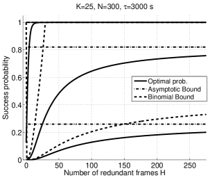
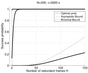
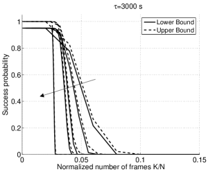
Figure 1: a) Success probability for $N=300$, $K=25$, $p=1$ under different values of $\lambda$; $\lambda_{1}=0.22\cdot 10^{-03}s^{-1}$, $\lambda_{2}=0.091\cdot 10^{-03}s^{-1}$ $\lambda_{3}=0.065\cdot 10^{-03}s^{-1}$ b) Success probability for $\lambda_{1}$, $N=300$, $p=1$ under different values of $K$ c) Upper and lower bound $p=1$, $\delta=0.02$ as given in Cor. IV.1, for various values of $N=50,125,300,500,5000$, versus normalized number of transmitted frames $K/N$.

We add $H$ redundant frames and consider the new message that now contains $K+H$ frames. If at time $t$ the source encounters a mobile which does not have any frame, it gives it frame $i$ with probability $p$.

Let $S_{n,p}$ be a binomially distributed r.v. with parameters $n$ and $p$, i.e.

$$P(S_{n,p}=m)=B(p,n,m):={n\choose m}p^{m}(1-p)^{n-m}$$

The probability of a successful delivery of the message by time $\tau$ is thus

$$P_{s}(\tau,K,H)=\sum_{j=K}^{K+H}B(D_{i}(\tau),K+H,j),$$

where $D_{i}(\tau)=1-\exp(-\lambda\int_{0}^{\tau}X_{i}(s)ds)$.

III-A Main Result

Lemma III.1

The maximum of $P_{s}(\tau,K,H)$ over $\{p_{m}\geq 0,m=1,...,K+H\}$ under the constraint $\sum_{i=1}^{K+H}p_{i}=p$ is achieved at $p_{m}=p/(K+H)$.

The proof is delayed to the Appendix.

Using the same arguments as those that led to Theorem II.2, together with Lemma III.1 yields the following:

Theorem III.1

Consider the problem of maximizing $P_{s}(\tau,K,H)$ over $p_{i},i=1,...,K+H,$ subject to a constraint on the energy ${\cal E}(\tau)\leq\varepsilon x$.
(i) If $\overline{X}(\tau)\leq x+z$ (or equivalently, $\tau\leq\sigma(z)$), then a control policy $u$ is optimal if and only if $p_{i}=1/(K+H)$ for all $i$.
(ii) If $\overline{X}(u_{\min}\tau)>z+x$ (or equivalently, $u_{\min}\tau>\sigma(z)$), then there is no feasible control strategy.
(iii) If $\overline{X}(\tau)>z+x>\overline{X}(u_{\min}\tau)$ (or equivalently, $\tau>\sigma(z)>u_{\min}\tau$), then the best control policy is given by $p_{i}=p^{*}/(K+H)$ where $p^{*}$ is given in (10) and the optimal value is

$$P_{s}^{*}(\tau,K,H)=\sum_{j=K}^{K+H}B\left(\widehat{p},K+H,j\right)$$

where

$$\widehat{p}=1-\exp(L(p^{*},\tau)p^{*}/(K+H))$$

III-B Properties and Approximations

We now derive further characterizations for the optimal success probability; these results will provide both bounds for the case of block coding and help also in the analysis of fountain codes.

Corollary III.1

$P_{s}^{*}(\tau,K,H)$ is increasing with $H$.

Proof:

We make the following observation. Fix $K$ and $H$ and a vector $(p_{1},...,p_{K+H})$ whose entries sum up to $p^{*}$ (given in (10)). Then the success probability is the same as when increasing the redundancy to $H+1$ and using the vector $(p_{1},...,p_{K+H},0)$. By definition, the latter is strictly smaller than $P_{s}^{*}(\tau,K,H+1)$ (which is the optimal success probability with $H+1$ redundant packets).

The above is in particular true when taking $p_{i}=p^{*}/(K+H)$ (which maximizes $P_{s}(\tau,K,H)$), and hence $P_{s}^{*}(\tau,K,H)<P_{s}^{*}(\tau,K,H+1)$. ∎

Now we provide two useful bounds for $P_{s}^{*}(\tau,H,K)$.

First, it is possible to derive the asymptotic approximation of $P_{s}^{*}(\tau,H,K)$ for $H\rightarrow\infty$. For the sake of notation, let $V=L(p,\tau)p$; the following holds

$$P_{s}^{*}(\tau,H,K)=e^{V}\sum_{s=K}^{H+K}{{H+K}\choose s}\Big{(}e^{-\frac{V}{H+K}}-1\Big{)}^{s}$$

$$=1-e^{V}\sum_{s=0}^{K-1}{{H+K}\choose s}\Big{(}\frac{-V}{(H+K)^{s}}+o((H+K)^{-s})\Big{)}$$

For large values of $H+K$, the $s$-th term of the right-hand summation writes

$${{H+K}\choose s}\Big{(}\frac{-V}{H+K}\Big{)}^{s}=\frac{(H+K)!}{s!(H+K-s)!}\frac{(-V)^{s}}{(H+K)^{s}}$$

$$\sim\frac{(-V)^{s}}{s!e^{s}}\frac{1}{\Big{(}1-\frac{s}{H+K}\Big{)}^{H+K}}\sim\frac{(-V)^{s}}{s!}$$

where the Stirling formula applies, $n!\sim\sqrt{2\pi n}\;(\frac{n}{e})^{n}$, with $f\sim g$ meaning $\lim_{H\rightarrow\infty}f/g=1$.

Corollary III.2

For $K\geq 1$ and $\tau\geq 0$,

$$\lim_{H\rightarrow\infty}P_{s}^{*}(\tau,H,K)=1-e^{L(p,\tau)p}\sum_{s=0}^{K-1}\frac{[-L(p,\tau))p]^{s}}{s!}$$

We note that in sight of the monotonicity stated in Cor. III.1, the limit is reached from below.

Also, the binomial bound [15, Thm 1.1] applies. For $1\leq m\leq n-1$, and $u>1$, define $u$ through $m=\lceil upn\rceil$. Then

$$P(S_{n,p}\geq m)\leq\frac{n^{1/2}}{(2\pi m(n-m))^{1/2}}\frac{u^{1-upn}}{1-u}\left(\frac{1-p}{1-up}\right)^{(1-up)n}$$

In Fig 1a) we reported the numerical comparison of the optimal delivery probability as a function of the number of redundant frames, for a particular setting. The asymptotic bound is reported as an horizontal dot-slashed line; the binomial bound is reported with slashed line. We notice that the binomial bound proves a good approximation for lower success probabilities, i.e., at smaller values of $\lambda$. The relative increase of the success probability under erasure codes is apparent: for instance, the success probability with $\lambda=0.22\cdot 10^{-03}s^{-1}$ increases from $0.12$ for $H=0$ to one with a few redundant frames ($H=12$); the maximum attainable improvement, though, is dictated by the upper bound.

In Fig 1b) the optimal delivery probability is depicted as a function of the number of redundant frames, at the increase of $K$; even in this case the binomial bound proves a better approximation for lower success probabilities, as it appears in the case of $K=60$.

III-C Phase transition

In what follows we elaborate based on result from Thm. III.1, and we study the case of large values of $N$. Let us assume that the total number of frames, $H+K$, grows as a function of $N$, i.e., $H+K=(H+K)(N)$.

The question we would like to answer is, in the asymptotic regime, what is the effect of redundancy onto the delivery probability, that is, how the number of redundant frames should scale with respect to the total number of frames.

We assume throughout that the following limits exist:

$$\widehat{K}:=\lim_{N\rightarrow\infty}K(N)/N\mbox{ and }\widehat{H}:=\lim_{N\rightarrow\infty}H(N)/N$$

Notice that this implies of course that the energy constraint should grow at most linearly with $N$ and we thus assume that the limit $\widehat{x}:=\lim_{N\rightarrow\infty}x(N)/N>0$ exists .

Proposition III.1

Introduce the threshold

$$\Gamma_{0}:=\lambda\tau\Big{(}1+\frac{\widehat{x}}{\log(1-\widehat{x})}\Big{)},$$

then, the following holds:
$\begin{array}[]{c}\lim_{N\rightarrow\infty}P_{s}(\tau,K,H)=\begin{cases}0&\mbox{if}\ \widehat{K}+\widehat{H}\leq\Gamma_{0}\\[5.69054pt] 0&\displaystyle\mbox{if}\ \widehat{K}+\widehat{H}>\Gamma_{0}\ \mbox{and}\ \widehat{K}>\Gamma_{0}\\[5.69054pt] 1&\mbox{if}\ \displaystyle\widehat{K}+\widehat{H}>\Gamma_{0}\ \mbox{and}\ \widehat{K}<\Gamma_{0}\end{cases}\end{array}$

The proof is in the Appendix. We conclude that there exist a phase-transition effect. Its threshold $\Gamma_{0}$ is the same as that we shall obtain later for the fountain codes.

The way we interpret such result is that, in order to deliver with high probability the message, for large $N$, the $K$ message frames should not exceed such threshold, but the sum of the encoded ones should.

IV Fountain Codes

Each time the source meets a node, it sends to it (with probability $p$) a packet obtained by generating a new random linear combination of the $K$ original packets. Using fountain codes, we know that for any $\delta$ in order for the destination to be able to decode the original message with probability at least $1-\delta$, it has to receive at least $M:=K\log(K/\delta)$ packets [16, Chap 50]. A useful expression for large $K$ will be used later: if we write $M=K(1+\alpha)$ then $\alpha$ that guarantees that the destination can decode the original message with probability of at least $1-\delta$ is given by

$$\alpha=\frac{(\log(K/\delta))^{2}}{\sqrt{K}}$$

The number of packets that reach the destination during the time interval $[0,\tau]$ has a Poisson distribution with parameter $-L(\tau,p^{*})p^{*}$ where $p^{*}$ is given in (10) and where $L(\tau,p^{*})$ is given in (9).

The probability that less than $M$ packets reach the destination is given by

$$P_{M}(\tau)=\sum_{i=0}^{M-1}\frac{(-L(\tau,p^{*})p^{*})^{i}}{i!}\exp(L(\tau,p^{*})p^{*})$$ (11)

We conclude that $P_{s}^{*}(\tau)\geq 1-\delta-P_{M}(\tau).$

Finally, we can leverage Cor. III.2 and obtain

Corollary IV.1

Given $p^{*}$ as in (10),

$$1-\delta-P_{M}(\tau)\leq P_{s}^{*}(\tau)\leq 1-P_{M}(\tau)$$

We notice that the bound on the right-end of the inequality is obtained by using redundancy as in the previous section for $H\geq M$, then taking the limit of $H\rightarrow\infty$.

IV-A Numerical examples: a phase transition

In Fig 1c) we reported the representation of the bounds described above: the two bounds provide a tight characterization of the performances of fountain codes; in particular, we notice that $P_{M}(\tau)$, which in fact is the CDF of a Poisson r.v., tends to one as $K$ increases: this causes the success probability to tend to zero as $K$ increases. The intuition is that, for a large number of transmitted frames, the probability of receiving all of them successfully within the given deadline decreases faster than the gain obtained by adding redundancy through fountain codes.

But, the numerical insight of the model says more of the performance attained by fountain codes. In fact, in Fig 1c) we reported $P_{s}^{*}$ versus the normalized number of transmitted frames $K/N$, for increasing $N$. Interestingly, the success probability becomes more and more close to a step function at the increase of $N$. We thus observe a phase transition: above a given number of transmitted frames, the success probability vanishes, and below the same threshold success occurs with probability one.

We shall study this phenomenon analytically in the next subsection.

IV-B Analysis Asymptotic behavior

We now want to understand the behavior of the fountain codes for large values of $N$ in the asymptotic regime $K=K(N)\leq N$; in what follows, we will assume that $\widehat{K}:=\lim_{N\rightarrow\infty}K(N)/N$ exists. This implies of course that the energy constraint should grow linearly with $N$ and we thus assume that the limit $\widehat{x}:=\lim_{N\rightarrow\infty}x(N)/N$ exists. We can rewrite $-L(\tau,p^{*})p^{*}=N\cdot\Gamma_{0}^{(0)}$, where we obtain

$$\Gamma_{0}^{(N)}=-\frac{1}{p^{*}}\Big{(}1-\lambda p^{*}\tau-e^{-\lambda p^{*}\tau}\Big{)}=\lambda\tau\Big{(}1+\frac{\frac{x}{N-z}}{\log(1-\frac{x}{N-z})}\Big{)}$$

$$\Gamma_{0}:=\lim_{N\to\infty}\Gamma_{0}^{(N)}=\lambda\tau\Big{(}1+\frac{\widehat{x}}{\log(1-\widehat{x})}\Big{)}$$

We have

$$P_{M}^{(N)}(\tau)=\sum_{i=0}^{K(N)(1+\alpha)-1}\frac{(N\cdot\Gamma_{0}^{(N)})^{i}}{i!}\exp(-N\cdot\Gamma_{0}^{(N)})$$

We notice that $P_{M}^{(N)}(\tau)=Pr\{X_{N}\leq K(N)(1+\alpha)-1\}$, where $X_{N}$ is a Poisson r.v. From the Strong Law of Large Numbers we have $\lim_{N\to\infty}{X_{N}}/{N}=\Gamma_{0}$ P-a.s. Thus

$$\lim_{N\to\infty}P_{M}^{(N)}(\tau)=1-\lim_{N\to\infty}Pr({X_{N}}\geq K(N))$$

$$=\begin{cases}1,&\mbox{if}\quad\widehat{K}>\Gamma_{0}\\ 0,&\mbox{if}\quad\widehat{K}<\Gamma_{0}\end{cases}$$

from which we can deduce

$\lim_{N\rightarrow\infty}P_{s}(\tau)\begin{cases}\geq 1-\delta,&\mbox{if}\quad\widehat{K}<\Gamma_{0}\\ =0,&\mbox{if}\quad\widehat{K}>\Gamma_{0}\end{cases}$

where we used Cor. IV.1.

This demonstrates the effect of phase transition observed numerically in Fig 1c).

V Threshold policies

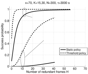
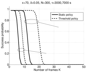
Figure 2: A comparison of success probability with erasure codes when using threshold and static policies; $N=300$, $x=70$, $\tau=3000,7000$: a) Erasure Codes, $K=15,30$ b) Fountain codes, $\delta=0.05$.

The way the energy constraints are handled so far is by using only a fraction of the transmission opportunities. This was done uniformly in time by transmitting at a probability that is time independent; we will refer to this strategy as static policy. In this section we consider an alternative way to distribute the transmissions: we use every possible transmission opportunity till some time limit and then stop transmitting. This is motivated by the ”spray and wait” policy [17] that is known to trade off very efficiently message delay and number of replicas in case of a single message.

In addition we need to specify the values of $p_{i}$: the probability packet $i$ when there is an opportunity to transmit (and the time limit has not yet elapsed). We have $\sum_{i=1}^{K}p_{i}=1$.

In the lack of redundancy, we recall that the success probability writes

$$P_{s}(\tau,{\bf p})=\prod_{i=1}^{K}\Big{(}1-\exp(-\lambda\int_{0}^{\tau}X_{i}(v)dv)\Big{)}$$

Clearly, transmitting always when there is an opportunity to transmit is optimal if by doing so the energy constraint are not violated. This can be considered to be a trivial time limit policy with a limit of $r=\tau$. Otherwise, the optimal value $r$ for a threshold is the one that achieves the energy constraints, or equivalently, the one for which the expected number of transmissions during time interval $[0,r]$ by the source is $x$; as before, $x$ is related to the total constraint on the energy through the constraint ${\cal E}(\tau)\leq\varepsilon x$. The value $r$ of the time limit is then given by $\sigma(z)$, see eq. (8).

Since we considered a time limit policy, $X_{i}(v)$ first grows till the time limit $r$ is reached and then it stays unchanged during the interval $(r,\tau]$. For the non-trivial case where $r=\sigma(z)$ we thus have:

$$P_{s}(\tau,{\bf p})=\prod_{i=1}^{K}\Big{[}1-\exp\Big{(}-{\lambda}\int_{0}^{\sigma(z)}N{p_{i}}\Big{(}1-e^{-\lambda v}\Big{)}dv$$

$$-\lambda(\tau-\sigma(z))X_{i}(\sigma(z))\Big{)}\Big{]}=\prod_{i=1}^{K}\tilde{Z}(p_{i})$$

where $\tilde{Z}(p_{i}):=1-\exp\Big{(}p_{i}\tilde{L}(\tau)\Big{)},$ $p_{i}\tilde{L}(\tau):=-\lambda\,\int_{0}^{\tau}X_{i}(v)dv$ and where we have by eq. (5) and (8)

$$X_{i}(\sigma(z))=Np_{i}\Big{(}1-e^{-\lambda\sigma(z)}\Big{)}=\frac{Np_{i}x}{N-z}$$

Also, the integral can be expressed as

$$\int_{0}^{\sigma(z)}X_{i}(v)dv=-\frac{Np_{i}}{\lambda}\left[-\frac{x}{N-z}+\log\Big{(}1-\frac{x}{N-z}\Big{)}\right]$$

In particular, the following holds

$$\tilde{L}(\tau)=\frac{Nx}{N-z}+N\log\Big{(}1-\frac{x}{N-z}\Big{)}-\lambda(\tau-\sigma(z))\frac{Nx}{N-z}$$

$$=-\frac{Nx}{N-z}\lambda\tau-\beta(z)\mbox{, \qquad where}$$

$$\beta(z)=-\frac{Nx}{N-z}-N\Big{(}1-\frac{x}{N-z}\Big{)}\log\Big{(}1-\frac{x}{N-z}\Big{)}\geq 0.$$

Finally, the $p_{i}$’s are selected to be all equal (and to sum to 1) due to the same arguments as in the proof Theorem II.1 as here too, $\log(\tilde{Z})$ is concave in its argument.

In the case of redundancy, the calculations are similar to those in eq. (V), where

$$P_{s}(\tau,H,K)=\sum_{s=K}^{H+K}{{H+K}\choose s}\tilde{Z}^{s}(p_{i})(1-\tilde{Z}(p_{i}))^{N-s}$$ (12)

Hence, given $H\geq 0$, it holds

$$P_{s}^{*}(\tau,H,K)=\exp\left(-\frac{\frac{Nx}{N-z}\lambda\tau+\beta(z)}{H+K}\right)$$

$$\times \sum_{s=K}^{H+K}{{H+K}\choose s}\left[\exp\left(\frac{\frac{Nx}{N-z}\lambda\tau+\beta(z)}{H+K}\right)-1\right]^{s}$$

Here again, we used the fact that the success probability is maximized for equal $p_{i}$’s, i.e.

$$p_{i}^{*}(t)=\begin{cases}1/(H+K)&\quad{\mbox{if}}\quad t\leq\sigma(z)\\ 0&\quad{\mbox{if}}\quad t>\sigma(z)\end{cases}$$

and $P_{s}^{*}(\tau,H,K)$ is given as in eq. (V). The proof follows the same lines as that of Lemma III.1.

As a final remark, consider the trivial case where the energy constraint is not active: $\tau<\sigma(z)$, i.e., it is optimal to transmit all the $x$ packets up to time $\tau$; in this case results from Thm. III.1 hold.

Now we want to specialize the use of threshold policies in the case of fountain codes when the energy constraint is active: $\tau\geq\sigma(z)$. In this case, the number of packets that reach the destination during the time interval $[0,\tau]$ has a Poisson distribution with parameter $\Lambda=-\tilde{L}(\tau)=\frac{Nx}{N-z}\lambda\tau+\beta(z)$; the probability that less than $M=K\log(K)$ packets reach the destination is given by

$$P_{M}(\tau)=\exp\left({-\frac{Nx}{N-z}\lambda\tau-\beta(z)}\right)\sum_{i=0}^{M-1}\frac{1}{i!}\Big{(}\frac{Nx}{N-z}\lambda\tau+\beta(z)\Big{)}^{i}$$

and the statement of Cor. IV.1 holds accordingly (notice that when the energy constraint is not active, we fall back to the original form of Cor IV.1).

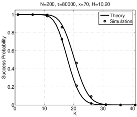
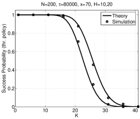
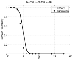
Figure 3: a) Simulation results for the success probability of erasure coded messages, static policy, $H=10,20$, $N=200$, $\tau=80000$ s, $x=70$. b) Same as a) but under threshold policies c) Simulation results for the success probability of fountain coded messages, static policy, $N=200$, $\tau=80000$ s, $x=70$, $\delta=0.02$.

V-A Comparison with static policies

Here we would like to see what is the relative performance of static and threshold policies, both for fountain codes and erasure codes. In Fig. 2a) and Fig. 2b) we reported on the case a bound on energy exists $x=70$; in such case, $\sigma(z)=1000$ s. As concerns erasure codes, when the number of frames is high ($30$) the usage of a large number of redundant frames proves much more effective compared to static policies. Conversely, a for a lower number of frames, the advantage of threshold policies is less marked.

In the case of fountain codes, threshold policies are again more efficient than static policies, and the effect is more relevant for large values of the time constraint $\tau$. We recall that we refer to optimal static policies.

VI Numerical Validation

In this section we provide a numerical validation of the model. Our experiments are trace based; message delivery is simulated by a Matlab${}^{\mbox{\scriptsize\textregistered}}$ script receiving as input pre-recorded contact traces.

Synthetic Mobility

We considered first a Random Waypoint (RWP) mobility model [18]. We registered a contact trace using Omnet++ with $N=200$ nodes moving on a squared playground of side $5$ Kms. The communication range is $R=15$ m, the mobile speed is $v=5$ m/s and the system starts in steady-state conditions in order to avoid transient effects [19]. The time limit is set to $\tau=80000$ s, which corresponds roughly to $1$ day operations, and the constraint on the maximum number of copies is $x=70$. With this first set of measurements, we want to check the fit of the model for the erasure codes and fountain codes. In the case of erasure codes, we fixed $H=10$ and $20$ and increased the number of message frames $K$. We selected at random pairs of source and destination nodes and registered the sample probability that the message is received at the destination by time $\tau$. As seen in Fig. 3a) the fit with the model is rather tight and an abrupt transition from high success probability to zero is visible. Also, in Fig. 3b) we reported on the results obtained in case of threshold policies; the fit is similar to what obtained for static policies, confirming the gain of performance with respect to static policies.

We repeated the same experiment in the case of fountain codes, as reported in Fig. 3c) for static policies; in this case the code specific parameter is $\delta=0.02$ and again we increased $K$. Even in this case we see that the threshold effect predicted by the model is apparent.

Real World traces

Our model captures the behavior of a sparse mobile ad hoc network under some assumptions: the most stringent is the uniformity and the stationarity of intermeeting intensities. We would like now to understand what is the impact of non-uniform and non-stationary encounter patterns. We considered two sets of experimental contact traces:

Haggle: in [2] and related works, the authors report extensive experimentation conducted in order to trace the meeting pattern of mobile users. A version of iMotes, equipped with a Bluetooth radio interface, was distributed to a number of people, each device collecting the time epoch of meetings with other Bluetooth devices. In the case of Haggle traces, due to the presence of several spurious contacts with erratic Bluetooth devices, we restricted the contacts to a subset having experienced at least $50$ contacts, resulting in $19$ active nodes.

CN: the CN dataset has been obtained by monitoring $21$ employee within Create-Net and working on different floors of the same building during a $4$-week period. Employees volunteered to carry a mobile running a Java application relying on Bluetooth connectivity. The application periodically triggers (every $60$ seconds) a Bluetooth node discovery; detected nodes are recorded via their Bluetooth address, together with the current timestamp on the device storage for a later processing.

Fig 4 a) and b) depict the results of experiments performed with these data sets. A major impact is played by the non-stationarity of traces. This is mainly due to “holes” appearing in the trace which impose unavoidable cutoff effects on the success probability. In particular, in the case of fountain coding, for $K>1$, i.e., when the original file is actually fragmented, the performance is rather poor. This is due to the increase with $K$ of the number of frames $M$ required for decoding, exacerbated by the reduced size of the network. For example, for $K=3$ and $\delta=0.05$ it holds $M=13$, i.e. $M$ is close to $N$ for the Haggle trace and larger than $N/2$ for the CN trace; this means that, in order to deliver the message, basically almost all nodes should meet the destination and deliver a frame within $\tau$.

With erasure codes, both traces show the characteristic cutoff of performances at the increase of $K$. The decay, though, depends on the trace considered; in particular, a close look to the two data sets showed that the Haggle trace has higher average inter-meeting intensity compared to the CN trace over the considered interval; the shape seen in Fig 4a) resembles more closely the theoretical sigmoid cutoff predicted by the model.

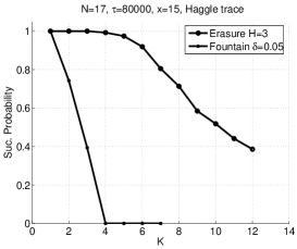
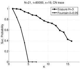
Figure 4: a) Simulation results for the success probability of static policies, Haggle trace, $N=17$, $\tau=80000$ s, $x=17$ and $\delta=0.05$ b) Simulation results for the success probability of static policy, CN trace, $N=21$, $\tau=80000$ s, $x=17$ and $\delta=0.05$.

VII Conclusions and Remarks

We have considered in this paper the tradeoff between energy and probability of successful delivery in presence of finite duration of contacts or limited storage capacity at a node: it can store only part (a frame) of a file that is to be transferred. To improve performance we considered the generation of erasure codes at the source which allows the DTN to gain in spatial storage diversity. Both fixed erasure codes (Reed Solomon type codes) as well as rateless fountain codes have been studied.

Fountain codes can be viewed as special case of general network coding such as those studied in [10, 7, 8]. We note however that in order to go beyond fountain codes (in which coding is done at the source) and consider general network coding (where coding is also done in the relay nodes), one needs not only change the coding approach but one should allow storage of several frames at each relay node. Also, interesting hints come from the presence of non-stationary patterns arising in real world traces. New tradeoff issues arise which we shall study in future work.

VIII Appendix

VIII-A Proof of Theorem II.1.

Proof:

The case $p=0$ is trivial so we assume below $p>0$. We have

$$P_{s}^{*}(\tau) = \max_{{\bf p}:\sum_{i}p_{i}=p}P_{s}(\tau)=\max_{{\bf p}:\sum_{i}p_{i}=p}\prod_{i=1}^{K}Z(p_{i})$$

${\bf p^{*}}$ is optimal if and only if it maximizes $g({\bf p}):=\sum_{i=1}^{K}\log(Z(p_{i}))$ s.t. $\sum_{i}p_{i}=p$, $p_{i}\geq 0$. Note that $L(\tau)$ is non-positive. $\log Z$ turns out to be a concave function. It then follows from Jensen’s inequality that

$$g({\bf p}) = \frac{1}{K}\sum_{i=1}^{K}\log(Z(p_{i}))$$ (14)

$$\leq \log\Big{(}Z\Big{(}\frac{1}{K}\sum_{i=1}^{K}p_{i}\Big{)}\Big{)}=\log\Big{(}Z\Big{(}\frac{p}{K}\Big{)}\Big{)}$$

where equality is attained for $p_{i}=p/K$. This concludes the proof.∎

VIII-B Proof of Lemma III.1

Proof:

Let $A(K,H)$ be the set of subsets $h\subset\{1,...,K+H\}$ that contain at least $K$ elements. For example, $\{1,2,...,K\}\in A(K,H)$. Fix $p_{i}$ such that $\sum_{i=1}^{K+H}p_{i}=p$. Then the probability of successful delivery by time $\tau$ is given by

$$P_{s}(\tau,K,H)=\sum_{h\in A(H,K)}\prod_{i\in h}Z(p_{i})$$

For any $i$ and $j$ in $\{1,...,K+H\}$ we can write

$$P_{s}(\tau,K,H)=Z(p_{i})Z(p_{j})g_{1}+(Z(p_{1})+Z(p_{2}))g_{2}+g_{3}$$

where $g_{1}$, $g_{2}$ and $g_{3}$ are nonnegative functions of $\{Z(p_{m}),m\not=i,m\not=j\}$. For example,

$$g_{1}=\sum_{h\in A_{\{i,j\}}(H,K)}\prod_{\stackrel{{\scriptstyle m\in h}}{{m\not=i}},\;{m\not=j}}Z(p_{m})$$

where $A_{v}(K,H)$ is the set of subsets $h\subset\{1,...,K+H\}$ that contain at least $K$ elements and such that $v\subset h$.

Now consider maximizing $P_{s}(\tau,K,H)$ over $p_{i}$ and $p_{j}$ that satisfy $p^{\prime}=p_{i}+p_{j}$ for a given $p^{\prime}\leq p$. Since $Z(\cdot)$ is strictly concave, it follows by Jensen’s inequality that $Z(p_{i})+Z(p_{j})$ has a unique maximum at $p_{i}=p_{j}=p^{\prime}/2$. This is also the unique maximum of the product $Z(p_{i})Z(p_{j})$ (using the same argument as in eq. (14)), and hence of $P_{s}(\tau,K,H)$.

Since this holds for any $i$ and $j$ and for any $p^{\prime}\leq p$, this implies the Lemma.∎

VIII-C Proof of Proposition III.1

Proof:

From Thm. III.1,

$$P_{s}^{*}(\tau,K,H)=P\{S_{H+K,\widehat{p}}\leq H+K\}-P\{S_{H+K,\widehat{p}}<K\},$$

where $\widehat{p}=1-\exp\Big{(}\frac{L(p^{*},\tau)p^{*}}{H+K}\Big{)}$.

We can rewrite $-L(\tau,p^{*})p^{*}=N\cdot\Gamma_{0}^{(0)}$, where we obtain

$$\Gamma_{0}^{(N)}=-\frac{1}{p^{*}}\Big{(}1-\lambda p^{*}\tau-e^{-\lambda p^{*}\tau}\Big{)}=\lambda\tau\Big{(}1+\frac{\frac{x}{N-z}}{\log(1-\frac{x}{N-z})}\Big{)}$$

and we define

$$\Gamma_{0}:=\lim_{N\to\infty}\Gamma_{0}^{(N)}=\lambda\tau\Big{(}1+\frac{\widehat{x}}{\log(1-\widehat{x})}\Big{)}$$

Notice also that,

$$E[S_{H+K,\widehat{p}}] = (H+K)\widehat{p}=(H+K)\Big{(}1-e^{-\frac{N\Gamma_{0}^{(N)}}{H+K}}\Big{)}$$

$$= (H+K)\Big{(}\frac{N\Gamma_{0}^{(N)}}{H+K}+o\big{(}\frac{1}{H+K}\big{)}\Big{)}$$

from which it follows that

$$\lim_{N\rightarrow\infty}\frac{E[S_{H+K,\widehat{p}}]}{N} = \lim_{N\to\infty}(H+K)\widehat{p}/N=\Gamma_{0}$$

Notice that the binomial r.v. $S_{H+K,\widehat{p}}$ can be interpreted as the sum of $H+K$ independent binary random variables $i_{n}$ with mean $\widehat{p}$ and variance $\widehat{p}(1-\widehat{p})$. Also, the series of the normalized variances $\sigma^{2}_{i_{n}}=\frac{1}{n^{2}}\widehat{p}(1-\widehat{p})\leq\frac{1}{n^{2}}$ is finite. Thus, the Strong Law of Large Numbers [20] ensures that $\lim_{N\to\infty}{S_{H+K,\widehat{p}}}/{N}=\Gamma_{0}$ P-a.s.

Now we can derive

$$\lim_{N\to\infty}P\{S_{H+K,\widehat{p}}\leq H+K\}=\begin{cases}0,&\mbox{if}\quad\widehat{K}+\widehat{H}\leq\Gamma_{0}\\ 1,&\mbox{if}\quad\widehat{K}>\Gamma_{0}\end{cases}$$

and, in a similar way,

$$\lim_{N\to\infty}P\{S_{H+K,\widehat{p}}<K\}=\begin{cases}0,&\mbox{if}\quad\widehat{K}<\Gamma_{0}\\ 1,&\mbox{if}\quad\widehat{K}\geq\Gamma_{0}\end{cases}$$

Finally, by enumeration,

$$\lim_{N\to\infty}P_{s}(\tau,K,H)=\begin{cases}0&\mbox{if}\ \widehat{K}+\widehat{H}\leq\Gamma_{0}\\[5.69054pt] 0&\displaystyle\mbox{if}\ \widehat{K}+\widehat{H}>\Gamma_{0}\ \mbox{and}\ \widehat{K}\geq\Gamma_{0}\\[5.69054pt] 1&\mbox{if}\ \displaystyle\widehat{K}+\widehat{H}>\Gamma_{0}\ \mbox{and}\ \widehat{K}<\Gamma_{0}\end{cases}$$

This concludes the proof.∎

References

- [1] S. Burleigh, L. Torgerson, K. Fall, V. Cerf, B. Durst, K. Scott, and H. Weiss, “Delay-tolerant networking: an approach to interplanetary Internet,” IEEE Communications Magazine, vol. 41, pp. 128–136, June 2003.
- [2] A. Chaintreau, P. Hui, J. Crowcroft, C. Diot, R. Gass, and J. Scott, “Impact of human mobility on opportunistic forwarding algorithms,” IEEE Transactions on Mobile Computing, vol. 6, pp. 606–620, 2007.
- [3] T. Spyropoulos, K. Psounis, and C. Raghavendra, “Efficient routing in intermittently connected mobile networks: the multi-copy case,” ACM/IEEE Transactions on Networking, vol. 16, pp. 77–90, February 2008.
- [4] M. Grössglauser and D. Tse, “Mobility increases the capacity of ad hoc wireless networks,” IEEE/ACM Transactions on Networking, vol. 10, pp. 477–486, August 2002.
- [5] Y. Wang, S. Jain, M. Martonosi, and K. Fall, “Erasure-coding based routing for opportunistic networks,” in Proc. of SIGCOMM workshop on Delay-tolerant networking (WDTN). Philadelphia, Pennsylvania, USA: ACM, August 26 2005, pp. 229–236.
- [6] S. Jain, M. Demmer, R. Patra, and K. Fall, “Using redundancy to cope with failures in a delay tolerant network,” SIGCOMM Comput. Commun. Rev., vol. 35, no. 4, pp. 109–120, 2005.
- [7] C. Fragouli, J.-Y. L. Boudec, and J. Widmer, “Network coding: an instant primer,” SIGCOMM Comput. Commun. Rev., vol. 36, no. 1, pp. 63–68, 2006.
- [8] Y. Lin, B. Liang, and B. Li, “Performance modeling of network coding in epidemic routing,” in Proc. of MobiSys workshop on Mobile opportunistic networking (MobiOpp). San Juan, Puerto Rico: ACM, June 11 2007, pp. 67–74.
- [9] J. Widmer and J.-Y. L. Boudec, “Network coding for efficient communication in extreme networks,” in Proc. of the ACM SIGCOMM workshop on Delay-tolerant networking (WDTN), Philadelphia, Pennsylvania, USA, August 26 2005, pp. 284–291.
- [10] A. E. Fawal, K. Salamatian, D. C. Y. Sasson, and J. L. Boudec, “A framework for network coding in challenged wireless network,” in Proc. of MobiSys. Uppsala, Sweden: ACM, June 19-22 2006.
- [11] R. Groenevelt and P. Nain, “Message delay in MANETs,” in Proc. of SIGMETRICS. Banff, Canada: ACM, June 6 2005, pp. 412–413, see also R. Groenevelt, Stochastic Models for Mobile Ad Hoc Networks. PhD thesis, University of Nice-Sophia Antipolis, April 2005.
- [12] T. Karagiannis, J.-Y. L. Boudec, and M. Vojnović, “Power law and exponential decay of inter contact times between mobile devices,” in MobiCom. Montréal, Québec, Canada: ACM, September 9–14 2007, pp. 183–194.
- [13] E. Altman, T. Başar, and F. De Pellegrini, “Optimal monotone forwarding policies in delay tolerant mobile ad hoc networks,” in Proc. of ACM/ICST Inter-Perf. Athens, Greece: ACM, October 24 2008.
- [14] X. Zhang, G. Neglia, J. Kurose, and D. Towsley, “Performance modeling of epidemic routing,” Elsevier Computer Networks, vol. 51, pp. 2867–2891, July 2007.
- [15] B. Bollobás, Random Graphs. Cambridge University Press, 2001.
- [16] D. J. MacKay, Information Theory, Inference, and Learning Algorithms. Cambridge, UK: Cambridge University Press, 2003.
- [17] T. Spyropoulos, K. Psounis, and C. S. Raghavendra, “Spray and wait: an efficient routing scheme for intermittently connected mobile networks,” in Proc. of SIGCOMM workshop on Delay-tolerant networking (WDTN). Philadelphia, Pennsylvania, USA: ACM, 2005.
- [18] T. Camp, J. Boleng, and V. Davies, “A survey of mobility models for ad hoc network research,” Wireless Communications & Mobile Computing (WCMC), vol. 2, no. 5, pp. 483–502, August 2002.
- [19] J.-Y. L. Boudec and M. Vojnovic, “Perfect simulation and stationarity of a class of mobility models,” in Proc. of INFOCOM. Miami, USA: IEEE, March 13–17 2005, pp. 183–194.
- [20] W. Feller, Introduction to Probability Theory and Its Applications, 3rd ed. New York: Wiley, 1971.