Effects of high-order correlations on personalized recommendations for bipartite networks

Abstract

In this paper, we introduce a modified collaborative filtering (MCF) algorithm, which has remarkably higher accuracy than the standard collaborative filtering. In the MCF, instead of the cosine similarity index, the user-user correlations are obtained by a diffusion process. Furthermore, by considering the second-order correlations, we design an effective algorithm that depresses the influence of mainstream preferences. Simulation results show that the algorithmic accuracy, measured by the average ranking score, is further improved by 20.45% and 33.25% in the optimal cases of MovieLens and Netflix data. More importantly, the optimal value $\lambda_{\rm opt}$ depends approximately monotonously on the sparsity of the training set. Given a real system, we could estimate the optimal parameter according to the data sparsity, which makes this algorithm easy to be applied. In addition, two significant criteria of algorithmic performance, diversity and popularity, are also taken into account. Numerical results show that as the sparsity increases the algorithm considered the second-order correlation can outperform the MCF simultaneously in all three criteria.

, , , ,

1 Introduction

With the expansion of the Internet services, people are becoming increasingly dependent on the Internet with an information overload. Consequently, how to efficiently help people find information that they truly need is a challenging task nowadays [1]. Being an effective tool to address this problem, the recommender system has caught increasing attention and become an essential issue in Internet applications such as e-commerce system and digital library system [2]. Motivated by the practical significance to the e-commerce and society, the design of an efficient recommendation algorithm becomes a joint focus from engineering science to mathematical and physical community. Various kinds of algorithms have been proposed, such as correlation-based methods [3, 4], content-based methods [5, 6, 7, 8], spectral analysis [9, 10], iteratively self-consistent refinement [11], principle component analysis [12], network-based methods [13, 14, 15, 16], and so on. For a review of current progress, see Ref. [17, 18] and the references therein.

One of the most successful recommendation algorithms, called collaborative filtering (CF), has been developed and extensively investigated over the past decade [3, 4, 19]. When predicting the potential interests of a given user, such approach firstly identifies a set of similar users from the past records and then makes a prediction based on the weighted combination of those similar users’ opinions. Despite its wide applications, collaborative filtering suffers from several major limitations including system scalability and accuracy [20]. Recently, some physical dynamics, including mass diffusion (MD) [14, 15, 21] and heat conduction (HC) [13], have found their applications in personalized recommendations. Based on MD and HC, several effective network-based recommendation algorithms have been proposed [13, 14, 15, 16]. These algorithms have been demonstrated to be of both high accuracy and low computational complexity. However, the algorithmic accuracy and computational complexity may be very sensitive to the statistics of data sets. For example, the algorithm presented in Ref. [15] runs much faster than the standard CF if the number of users is much larger than that of objects, while when the number of objects is huge, the advantage of this algorithm vanishes because its complexity is mainly determined by the number of objects (see Ref. [15] for details). Since the CF algorithm has been extensively applied in the real e-commerce systems [4, 22], it’s meaningful to find some ways to increase the algorithmic accuracy of CF. We therefore present a modified collaborative filtering (MCF) method, in which the user correlation is defined based on the diffusion process. Recently, Liu et al. [23] studied the user and object degree correlation effect to CF, they found that the algorithm accuracy could be remarkably improved by adjusting the user and object degree correlation. In this paper, we argue that the high-order correlations should be taken into account to depress the influence of mainstream preferences and the accuracy could be improved in this way. The correlation between two users is, in principle, an integration of many underlying similar tastes. For two arbitrary users, the very specific yet common tastes shall contribute more to the similarity measure than those mainstream tastes. Figure 1 shows an illustration of how to find the specific tastes by eliminating the mainstream preference. To the users $A$ and $C$, the commonly selected objects 1 and 2 could reflect their tastes, where 1 denotes the mainstream preference shared by all $A$, $B$ and $C$, and 2 is the specific taste of $A$ and $C$. Both 1 and 2 contribute to the correlation between $A$ and $C$. Since 1 is the mainstream preference, it also contributes to the correlations between $A$ and $B$, as well as $B$ and $C$. Tracking the path $A\rightarrow B\rightarrow C$, the mainstream preference 1 could be identified by considering the second-order correlation between $A$ and $C$. Statistically speaking, two users sharing many mainstream preferences should have high second-order correlation, therefore we can depress the influence of mainstream preferences by taking into account the second-order correlation. The numerical results show that the algorithm involving high-order correlations is much more accurate and provides more diverse recommendations.

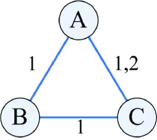
Figure 1: Illustration of the user correlation network. The users $A$, $B$ and $C$ are correlated because they have collected some common objects, where object $1$ has been collected by all of the three users, while object 2 is only collected by user $A$ and $C$.

2 Problem description and performance metrics

Denote the object set as $O=\{o_{1},o_{2},\cdots,o_{m}\}$ and the user set as $U$ = $\{u_{1},u_{2},$ $\cdots,$ $u_{n}\}$, a recommender system can be fully described by an adjacent matrix $A=\{a_{ij}\}\in R^{m,n}$, where $a_{ij}=1$ if $o_{i}$ is collected by $u_{j}$, and $a_{ij}=0$ otherwise. For a given user, a recommendation algorithm generates an ordered list of all the objects he/she has not collected before.

To test the recommendation algorithmic accuracy, we divide the data set into two parts: one is the training set used as known information for prediction, and the other one is the probe set, whose information is not allowed to be used. Many metrics have been proposed to judge the algorithmic accuracy, including precision [17], recall [17], F-measure [3], average ranking score [15], and so on. Since the average ranking score does not depend on the length of recommendation list, we adopt it in this paper. Indeed, a recommendation algorithm should provide each user with an ordered list of all his/her uncollected objects. For an arbitrary user $u_{i}$, if the entry $u_{i}$-$o_{j}$ is in the probe set (according to the training set, $o_{j}$ is an uncollected object for $u_{i}$), we measure the position of $o_{j}$ in the ordered list. For example, if there are $L_{i}=100$ uncollected objects for $u_{i}$, and $o_{j}$ is the 10th from the top, we say the position of $o_{j}$ is $10/100$, denoted by $r_{ij}=0.1$. Since the probe entries are actually collected by users, a good algorithm is expected to give high recommendations, leading to small $r_{ij}$. Therefore, the mean value of the position $r_{ij}$, $\langle r\rangle$ (called average ranking score [15]), averaged over all the entries in the probe, can be used to evaluate the algorithmic accuracy: the smaller the ranking score, the higher the algorithmic accuracy, and vice verse. For a null model with randomly generated recommendations, $\langle r\rangle=0.5$.

Besides accuracy, the average degree of all recommended objects, $\langle k\rangle$, and the mean value of Hamming distance, $S$, are taken into account to measure the algorithmic popularity and diversity [16]. The smaller average degree, corresponding to the less popular objects, are preferred since those lower-degree objects are hard to be found by users themselves. In addition, the personal recommendation algorithm should present different recommendations to different users according to their tastes and habits. The diversity can be quantified by the average Hamming distance, $S=\langle H_{ij}\rangle$, where $H_{ij}=1-Q_{ij}/L$, $L$ is the length of recommendation list, and $Q_{ij}$ is the overlapped number of objects in $u_{i}$’s and $u_{j}$’s recommendation lists. The higher $S$ indicates a more diverse and thus more personalized recommendations.

3 Modified collaborative filtering algorithm based on diffusion process

In the standard CF, the correlation between $u_{i}$ and $u_{j}$ can be evaluated directly by the well-known cosine similarity index

$$s_{ij}^{c}=\frac{\sum_{l=1}^{m}a_{li}a_{lj}}{\sqrt{k(u_{i})k(u_{j})}},$$ (1)

where $k(u_{i})=\sum_{l=1}^{m}a_{li}$ is the degree of user $u_{i}$. Inspired by the diffusion process presented by Zhou et al. [15], the user correlation network can be obtained by projecting the user-object bipartite network. How to determine the edge weight is the key issue in this process. We assume a certain amount of resource (e.g., recommendation power) is associated with each user, and the weight $s_{ij}$ represents the proportion of the resource $u_{j}$ would like to distribute to $u_{i}$. This process could be implemented by applying the network-based resource-allocation process [24] on a user-object bipartite network where each user distributes his/her initial resource equally to all the objects he/she has collected, and then each object sends back what it has received to all the users who collected it, the weight $s_{ij}$ (the fraction of initial resource $u_{j}$ eventually gives to $u_{i}$) can be expressed as:

$$s_{ij}=\frac{1}{k(u_{j})}\sum^{m}_{l=1}\frac{a_{li}a_{lj}}{k(o_{l})},$$ (2)

where $k(o_{l})=\sum^{n}_{i=1}a_{li}$ denotes the degree of object $o_{l}$. For the user-object pair $(u_{i},o_{j})$, if $u_{i}$ has not yet collected $o_{j}$ (i.e., $a_{ji}=0$), the predicted score, $v_{ij}$, is given as

$$v_{ij}=\frac{\sum_{l=1}^{n}s_{li}a_{jl}}{\sum_{l=1}^{n}s_{li}}.$$ (3)

Based on the definitions of $s_{ij}$ and $v_{ij}$, given a target user $u_{i}$, the MCF algorithm is given as following

(i)

Calculating the user correlation matrix $\{s_{ij}\}$ based on the diffusion process, as shown in Eq. (2);

(ii)

For each user $u_{i}$, based on Eq. (3), calculating the predicted scores for his/her uncollected objects;

(iii)

Sorting the uncollected objects in descending order of the predicted scores, and those objects in the top will be recommended.

The standard CF and the MCF have similar process, and their only difference is that they adopt different measures of user-user correlation (i.e., $s_{ij}^{c}$ for the standard CF and $s_{ij}$ for MCF).

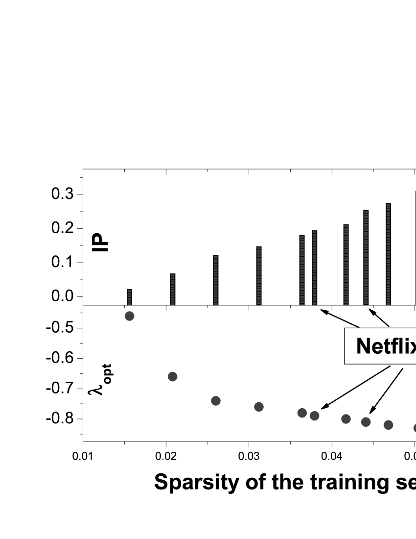
Figure 2: The optimal $\lambda_{\rm opt}$ and the improvement (IP) vs. the sparsity of the training sets. All the data points are averaged over ten independent runs with different data-set divisions. The results corresponding to Netflix data are marked.

4 Numerical results of MCF

We use two benchmark data sets, one is MovieLens, which consists of 1682 movies (objects) and 943 users. The other one is Netflix, which consists of 3000 movies and 3000 users (we use a random sample of the whole Netflix dataset). The users vote movies by discrete ratings from one to five. Here we applied a coarse-graining method [15, 16]: A movie is set to be collected by a user only if the giving rating is larger than 2. In this way, the MovieLens data has 85250 edges, and the Netflix data has 567456 edges. The data sets are randomly divided into two parts: the training set contains $p$ percent of the data, and the remaining $1-p$ part constitutes the probe.

Implementing the standard CF and MCF when $p=0.9$, the average ranking scores on MovieLens and Netflix data are improved from from 0.1168 to 0.1038 and from 0.2323 to 0.2151, respectively. Clearly, using the simply diffusion-based simlarity, subject to the algorithmic accuracy, the MCF outperforms the standard CF. The corresponding average object degree and diversity are also improved (see Fig.3 and Fig.4 below).

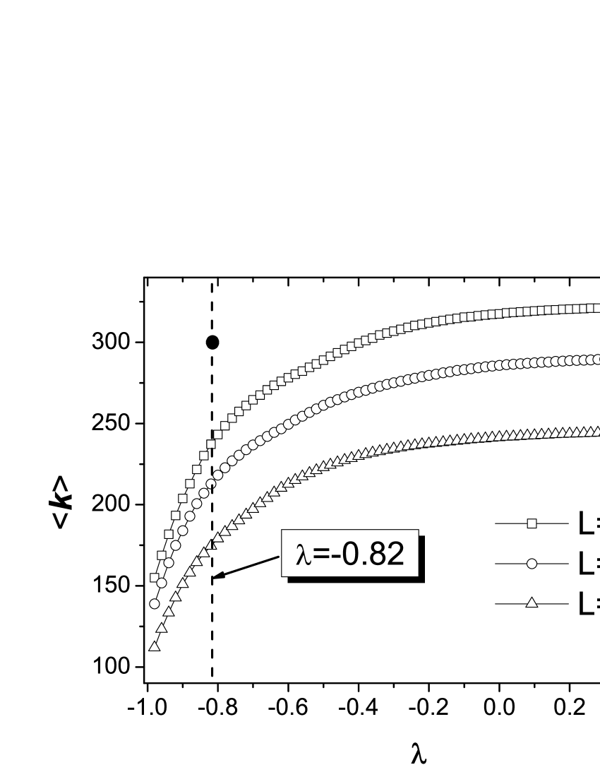
Figure 3: Average degree of recommended objects, $\langle k\rangle$, vs. $\lambda$ when $p=0.9$. Squares, circles and triangles represent lengths $L=10,20$ and $50$, respectively. The black point ($\bullet$) corresponds to the average degree obtained by the standard CF with $L=20$. All the data points are averaged over ten independent runs with different data-set divisions.

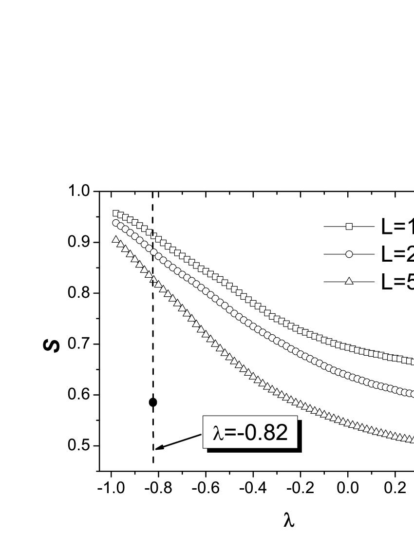
Figure 4: $S$ vs. $\lambda$ when $p=0.9$. Squares, circles and triangles represent the lengths $L=10,20$ and $50$, respectively. The black point ($\bullet$) corresponds to the diversity obtained by the standard CF with $L=20$. All the data points are averaged over ten independent runs with different data-set divisions.

5 Improved algorithm

To investigate the effect of second-order user correlation to algorithm performance, we use a linear form to investigate the effect of the second-order user correlation to MCF, where the user similarity matrix could be demonstrated as

$$\textbf{H}=\textbf{S}+\lambda\textbf{S}^{2},$$ (4)

where H is the newly defined correlation matrix, $\textbf{S}=\{s_{ij}\}$ is the first-order correlation defined as Eq. (2), and $\lambda$ is a tunable parameter. As discussed before, we expect the algorithmic accuracy can be improved at some negative $\lambda$.

When $p=0.9$, the algorithmic accuracy curves of MovieLens and Netflix have clear minimums around $\lambda=-0.82$ and $\lambda=-0.84$, which strongly support the above discussion. Compared with the routine case ($\lambda=0$), the average ranking scores can be further reduced to 0.0826 (improved 20.45%) and 0.1436( improved 33.25%) at the optimal values. It is indeed a great improvement for recommendation algorithms. Since the data sparsity can be turned by changing $p$, we investigate the effect of the sparsity on the two data sets respectively, and find that although we test the algorithm on two different data sets, the optimal $\lambda_{\rm opt}$ are strongly correlated with the sparsity in a uniform way for both MovieLens and Netflix. Figure 2 shows that when the sparsity increases, $\lambda_{\rm opt}$ will decrease, and the improvement of the average ranking scores will increase. These results can be treated as a good guideline for selecting optimal $\lambda$ of different data sets. Figure 3 reports the average degree of all recommended objects as a function of $\lambda$. One can see from Fig. 3 that when $p=0.9$ the average object degree is positively correlated with $\lambda$, thus to depress the influence of mainstream interests gives more opportunity to the less popular objects, which could bring more information to the users than the popular ones. When the list length, $L$, bing equal to 20, at the optimal point $\lambda_{\rm opt}=-0.82$, the average degree is reduced by 29.3% compared with the standard CF. When $p=0.9$, Fig. 4 exhibits a negative correlation between $S$ and $\lambda$, indicating that to consider the second-order correlations makes the recommendation lists more diverse. When $L=20$, the diversity $S$ is increased from 0.592 (corresponding to the standard CF) to 0.880 (corresponding to the case $\lambda=-0.82$ in the improved algorithm). Figure 3 and Figure 4 show how the parameter $\lambda$ affects the average object degree $\langle k\rangle$ and diversity $S$, respectively. Clearly, the smaller $\lambda$ leads to less popularity and higher diversity, and thus the present algorithm can find its advantage in recommending novel objects with diverse topics to users, compared with the standard CF. Generally speaking, the popular objects must have some attributes fitting the tastes of the masses of the people. The standard CF may repeatedly count those attributes and assign more power for the popular objects, which increases the average object degree and reduces the diversity. The present algorithm with negative $\lambda$ can to some extent eliminate the redundant correlations and give higher chances to less popular objects and the objects with diverse topics different from the mainstream [25].

Table 1: Algorithmic performance for MovieLens data when $p=0.9$. The precision, diversity and popularity are corresponding to $L=50$. NBI is an abbreviation of the network-based recommendation algorithm, proposed in Ref. [15]. Heter-NBI is an abbreviation of NBI with heterogenous initial resource distribution, proposed in Ref. [16]. CB-CF is an abbreviation of the correlation-based collaborative filtering method, proposed in Ref. [23]. Improved MCF is an abbreviation of the algorithm presented in this paper. The parameters in Heter-NBI and IMCF are set as the ones corresponding to the lowest ranking scores (for Heter-NBI [16], $\beta_{\texttt{opt}}=-0.80$; for CB-CF [23], $\lambda_{\texttt{opt}}=-0.96$; for IMCF, $\lambda_{\texttt{opt}}=-0.82$). Each number presented in this table is obtained by averaging over ten runs, each of which has an independently random division of training set and probe.

Algorithms	$\langle r\rangle$	$S$	$\langle k\rangle$
GRM	0.1390	0.398	259
CF	0.1168	0.549	246
NBI	0.1060	0.617	233
Heter-NBI	0.1010	0.682	220
CB-CF	0.0998	0.692	218
IMCF	0.0877	0.826	175

6 Conclusions

In this paper, a modified collaborative filtering algorithm is presented to improve the algorithmic performance. The numerical results indicate that the usage of diffusion based correlation could enhance the algorithmic accuracy. Furthermore, by considering the second-order correlations, $\textbf{S}^{2}$, we presented an effective algorithm that has remarkably higher accuracy. Indeed, when $p=0.9$ the simulation results show that the algorithmic accuracy can be further improved by 20.45% and 33.25% on MovieLens and Netflix data. Interestingly, we found even for different data sets, the optimal value of $\lambda$ exhibits a uniform tendency versus sparsity. Therefore, if we know the sparsity of the training set, the corresponding optimal $\lambda_{\rm opt}$ could be approximately confirmed. In addition, when the sparsity gets less than 1%, the improved algorithm wouldn’t be effective any more, while as the sparsity increases, the improvement of the presented algorithm is enlarged.

Ignoring the degree-degree correlation in user-object entries, The algorithmic complexity of MCF is $\textbf{O}(m\langle k_{u}\rangle\langle k_{o}\rangle+mn\langle k_{o}\rangle)$, where $\langle k_{u}\rangle$ and $\langle k_{o}\rangle$ denote the average degrees of users and objects. The first term accounts for the calculation of user correlation, and the second term accounts for the one of the predictions. It approximates to $\textbf{O}(mn\langle k_{o}\rangle)$ for $n\gg\langle k_{u}\rangle$. Clearly, the computational complexity of MCF is much less than that of the standard CF especially for the systems consisted of huge number of objects. In the improved algorithm, in order to calculate the second-order correlations, the diffusion process must flow from the user to the objects twice, therefore, the algorithmic complexity of the improved algorithm is $\textbf{O}(n\langle k_{u}\rangle^{2}\langle k_{o}\rangle^{2}+mn\langle k_{o}\rangle)$. Since the magnitude order of the object $m$ is always much larger than the ones of $\langle k_{u}\rangle$ and $\langle k_{o}\rangle$, the improved algorithm is also as comparably fast as the standard CF.

Beside the algorithmic accuracy, two significant criteria of algorithmic performance, average degree of recommended objects and diversity, are taken into account. A good recommendation algorithm should help the users uncovering the hidden (even dark) information, corresponding those objects with very low degrees. Therefore, the average degree is a meaningful measure for a recommendation algorithm. In addition, since a personalized recommendation system should provide different recommendations lists according to the user’s tastes and habits [2], diversity plays a crucial role to quantify the personalization [26, 27]. The numerical results show that the present algorithm outperforms the standard CF in all three criteria. How to automatically find out relevant information for diverse users is a long-standing challenge in the modern information science, we believe the current work can enlighten readers in this promising direction.

How to automatically find out relevant information for diverse users is a long-standing challenge in the modern information science, the presented algorithm also could be used to find the relevant reviewers for the scientific papers or funding applications [28, 29], and the link prediction in social and biological networks [30, 31]. We believe the current work can enlighten readers in this promising direction.

We acknowledge GroupLens Research Group for providing us the data. This work is partially supported by and National Basic Research Program of China (No. 2006CB705500), the National Natural Science Foundation of China (Nos. 10905052, 70901010, 60744003), the Swiss National Science Foundation (Project 205120-113842), and Shanghai Leading Discipline Project (No. S30501). T.Z. acknowledges the National Natural Science Foundation of China under Grant Nos. 10635040 and 60973069.

References

- [1] P. Resnick, H. R. Varian, Commun. ACM 40 (1997) 56.
- [2] J. B. Schafer, J. A. Konstan, J. Riedl, Data Min. & Knowl. Discovery 5 (2001) 115.
- [3] J. L. Herlocker, J. A. Konstan, K. Terveen, J. Riedl, ACM Trans. Inf. Syst. 22 (2004) 5.
- [4] J. A. Konstan, B. N. Miller, D. Maltz, J. L. Herlocker, L. R. Gordon, J. Riedl, Commun. ACM 40 (1997) 77.
- [5] M. Balabanović, Y. Shoham, Commun. ACM 40 (1997) 66.
- [6] M. J. Pazzani, Artif. Intell. Rev. 13 (1999) 393.
- [7] Y. Gao, H. Luo, J. Fan, Lect. Notes Comput. Sci. 5371 (2009) 217.
- [8] H. Luo, J. Fan, D. A. Keim, S. Satoh, Lect. Notes Comput. Sci. 5371 (2009) 459.
- [9] D. Billsus, M. Pazzani, Proc. Int’l Conf. Machine Learning, 1998, p. 46.
- [10] B. Sarwar, G. Karypis, J. A. Konstan, J. Riedl, Proc. ACM WebKDD Workshop at the ACM-SIGKDD Conf. on Knowledge Discovery in Databases, 2000.
- [11] J. Ren, T. Zhou, Y.-C. Zhang, Europhys. Lett. 80 (2008) 58007.
- [12] K. Goldberg, T. Roeder, D. Gupta, C. Perkins, Inform. Ret. 4 (2001) 133.
- [13] Y.-C. Zhang, M. Blattner, Y.-K. Yu, Phys. Rev. Lett. 99 (2007) 154301.
- [14] Y.-C. Zhang, M. Medo, J. Ren, T. Zhou, T. Li, F. Yang, Europhys. Lett. 80 (2008) 68003.
- [15] T. Zhou, J. Ren, M. Medo, Y.-C. Zhang, Phys. Rev. E 76 (2007) 046115.
- [16] T. Zhou, L.-L. Jiang, R.-Q. Su, Y.-C. Zhang, Europhys. Lett. 81 (2008) 58004.
- [17] G. Adomavicius, A. Tuzhilin, IEEE Trans. Know. & Data Eng. 17 (2005) 734.
- [18] J. -G. Liu, M. Z. Q. Chen, J. Chen, F. Deng, H. -T. Zhang, Z. Zhang, T. Zhou. Int. J. Inf. & Syst. Sci. 5(2) (2009) 230.
- [19] D. Sun, T. Zhou, J.-G. Liu, R.-R. Liu, C.-X. Jia, B.-H. Wang, Phys. Rev. E 80 (2009) 017101.
- [20] B. Sarwar, G. Karypis, J. A. Konstan, J. Reidl, Proc. ACM Conf. E-Commerce, 2000, p. 158.
- [21] J.-G. Liu, B.-H. Wang, Q. Guo, Int. J. Mod. Phys. C 20 (2009) 285.
- [22] G. Linden, B. Smith, J. York, IEEE Internet Computing, 7 (2003) 76.
- [23] J.-G. Liu, T. Zhou, Z.-G. Xuan, H.-A. Che, B.-H. Wang, Y.-C. Zhang, arXiv:0907.1228.
- [24] Q. Ou, Y.-D. Jin, T. Zhou, B.-H. Wang, B.-Q. Yin, Phys. Rev. E 75 (2007) 021102.
- [25] T. Zhou, R.-Q. Su, R.-R. Liu, L.-L. Jiang, B.-H. Wang, Y.-C. Zhang, arXiv: 0805.4127.
- [26] C. N. Ziegler, S. M. McNee, J. A. Konstan, G. Lausen, Proc. 14th Intl. Conf. WWW, 2005, p. 22.
- [27] T. Zhou, Z. Kuscsik, J.-G. Liu, M. Medo, J. Walkeling, Y.-C. Zhang, arXiv: 0808.2670.
- [28] J.-G. Liu, Y.-Z. Dang, Z.-T. Wang, Physica A 366 (2006) 578.
- [29] J.-G. Liu, Z.-G. Xuan, Y.-Z. Dang, Q. Guo, Z.-T. Wang, Physica A 377 (2007) 302.
- [30] T. Zhou, L. Lü, Y.-C. Zhang, Eur. Phys. J. B (to be published).
- [31] L. Lü, C.-H. Jin, T. Zhou, Phys. Rev. E (to be published).