On The Origins Of Eccentric Close-in Planets

Abstract

Strong tidal interaction with the central star can circularize the orbits of close-in planets. With the standard tidal quality factor $Q$ of our solar system, estimated circularization times for close-in extrasolar planets are typically shorter than the ages of the host stars. While most extrasolar planets with orbital radii $a\lesssim 0.1\,$AU indeed have circular orbits, some close-in planets with substantial orbital eccentricities have recently been discovered. This new class of eccentric close-in planets implies that either their tidal $Q$ factor is considerably higher, or circularization is prevented by an external perturbation. Here we constrain the tidal $Q$ factor for transiting extrasolar planets by comparing their circularization times with accurately determined stellar ages. Using estimated secular perturbation timescales, we also provide constraints on the properties of hypothetical second planets exterior to the known ones.

1. Introduction

The median eccentricity of the current sample of $\sim 300$ planets is 0.19, while it is 0.013 for close-in planets with semi-major axis $a<0.1\,$AU. The circular orbits of close-in planets most likely result from orbital circularization due to tides (e.g., Rasio et al., 1996; Marcy et al., 1997). This requires the tidal circularization time $\tau_{\rm circ}$ to be short compared to the age of the system $\tau_{\rm age}$. Since $\tau_{\rm circ}$ is a very steep function of $a$ (see Eq. 1 or 6), while $\tau_{\rm age}\sim 1-10\,$Gyr for most systems, a sharp decline in eccentricity is expected below some critical value of $a$. However, the observed transition seems to occur around $0.03-0.04\,$AU, whereas the calculated $\tau_{\rm circ}$ becomes comparable to $\tau_{\rm age}$ at $\sim 0.1\,$AU as we see below (Figure 1). Since almost one quarter (presently 16/68) of planets within $0.1\,$AU have $e>0.1$, their high eccentricities demand explanation.

First, we calculate the circularization times for transiting planets, and compare them with the estimated ages of the systems. The circularization time $\tau_{\rm circ}=-e/\dot{e}$, where $\dot{e}$ is the sum of the eccentricity change due to the tides raised on the star by the planet and those raised on the planet by the star, is (Goldreich & Soter, 1966; Hut, 1981; Eggleton et al., 1998; Mardling & Lin, 2002):

$$\tau_{\rm circ}=\frac{2}{81}\frac{Q_{\rm p}^{\prime}}{n}\frac{M_{\rm p}}{M_{*}}\left(\frac{a}{R_{\rm p}}\right)^{5}\left[\frac{Q_{\rm p}^{\prime}}{Q_{*}^{\prime}}\left(\frac{M_{\rm p}}{M_{*}}\right)^{2}\left(\frac{R_{*}}{R_{\rm p}}\right)^{5}F_{*}+F_{\rm p}\right]^{-1}\,$$ (1)

The subscripts p and $*$ represent the planet and star, respectively. The modified tidal quality factor for a planet is defined as $Q_{\rm p}^{\prime}\equiv 3Q_{\rm p}/2k_{\rm p}$, where $k_{\rm p}$ is the Love number, and $Q_{\rm p}$ is the specific dissipation function, which depends on the planetary structure as well as the frequency and amplitude of tides. We also define

$$F_{*} = \left[f_{1}(e^{2})-\frac{11}{18}f_{2}(e^{2})\frac{\Omega_{*,{\rm rot}}}{n}\right]$$ (2)

$$F_{\rm p} = \left[f_{1}(e^{2})-\frac{11}{18}f_{2}(e^{2})\frac{\Omega_{{\rm p,rot}}}{n}\right]\ ,$$ (3)

where $n=\sqrt{G(M_{*}+M_{\rm p})/a^{3}}$ is the mean motion, $\Omega_{\rm rot}$ is the rotational frequency, and

$$f_{1}(e^{2}) = \left(1+\frac{15}{4}e^{2}+\frac{15}{8}e^{4}+\frac{5}{64}e^{6}\right)/(1-e^{2})^{13/2},$$ (4)

$$f_{2}(e^{2}) = \left(1+\frac{3}{2}e^{2}+\frac{1}{8}e^{4}\right)/(1-e^{2})^{5}\ .$$ (5)

Generally $F_{*}$ and $F_{p}$ are comparable, and thus the stellar damping is negligible unless the planet-to-star mass (radius) ratio is large (small) or $Q_{*}^{\prime}\ll Q_{p}^{\prime}$. We define the circularization time due to damping in the planet as

$$\tau_{{\rm circ},0}=\frac{2}{81}\frac{Q_{\rm p}^{\prime}}{n}\frac{M_{\rm p}}{M_{*}}\left(\frac{R_{\rm p}}{a}\right)^{-5}F_{\rm p}^{-1}\ .$$ (6)

Note that $\tau_{{\rm circ},0}$ can be shorter or longer than $\tau_{{\rm circ}}$, depending on the sign of $F_{*}$, which changes at $(\Omega_{*,{\rm rot}}/n)_{\rm crit}=18/11(f_{1}/f_{2})$. In the limit $e\rightarrow 0$, this equation leads to the standard expression for the circularization time (Eq. 4.198 of Murray & Dermott, 1999).

Figure 1 compares the circularization times calculated from Eq. 1 and 6 with the estimated stellar ages for the systems in Table 1 . Here we assume $Q_{\rm p}^{\prime}=10^{5}$, and $Q_{*}^{\prime}=10^{6}$, which are the standard values motivated by measurements in our Solar System (e.g. Yoder & Peale, 1981; Zhang & Hamilton, 2008), and for main-sequence stars (e.g. Carone & Pätzold, 2007). For $\Omega_{\rm p,rot}$, we assume that planets with circular orbits are perfectly synchronized, i.e., $\Omega_{\rm p,rot}/n=1$, since the spin-orbit synchronization times are $\sim 10^{-3}\,\tau_{\rm circ}$ (Rasio et al., 1996). On the other hand, planets with eccentric orbits should spin down until they reach quasi-synchronization (Dobbs-Dixon et al., 2004); in practice we adopt a planetary spin frequency such that the rate of change of spin frequency is zero (Eq. 54 of Mardling & Lin, 2002). For the stellar spin, we assume typical periods derived from the observed $v_{\rm rot}\sin i$, $P_{*,{\rm rot}}\sim 3\,$– 70 d (Barnes, 2001).

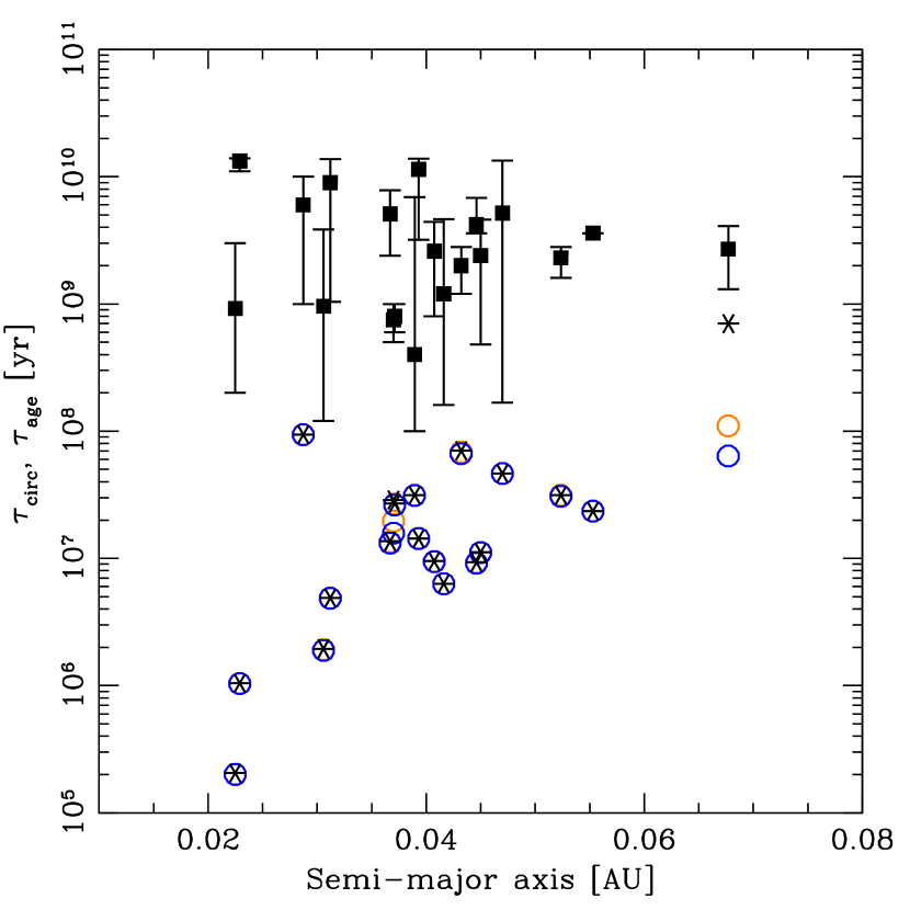
Figure 1.— Circularization times calculated from Eq. 6 (stars), Eq. 1 with $\Omega_{*,{\rm rot}}/n=3\,$d (orange circles) and 70 d (blue circles), compared with the estimated stellar ages (squares) for systems with transiting planets. Here we assume $Q_{\rm p}^{\prime}=10^{5}$ and $Q_{*}^{\prime}=10^{6}$. For all transiting planets, the estimated circularization time is shorter than the age of the host star.

Figure 1 compares the circularization times calculated from Eq. 1 and 6 with the estimated stellar ages for the systems in Table 1. For most systems the tidal damping in the star is negligible. Two systems with non-negligible stellar damping are WASP-14 and HAT-P-2. Both have a large planetary mass (see Table 1), and thus the first term in Eq. 1 is significant. Clearly, the estimated circularization times are always shorter than stellar ages, which implies that all these planets should have been circularized by now if their tidal $Q$ values were similar to those of their solar-system analogues. However, our sample contains at least 6 systems with a non-zero orbital eccentricity. Possible explanations are that (1) the structure of these planets is different and their actual $Q$ is greater than what we assumed; or (2) they currently experience external perturbations which maintain their orbital eccentricities against tidal dissipation.

2. Constraints on the Tidal $Q$ value of close-in planets

Now we use Eq. 1 to place constraints on the tidal $Q$ values of the planets. An upper limit on $Q$ is provided for planets with circular orbits since the circularization must have occurred within the lifetime of the systems ($\tau_{\rm circ}<\tau_{\rm age}$). Our assumption here is that these close-in planets formed through tidal circularization of initially eccentric orbits. Nagasawa et al. (2008) showed that about one third of multiple planetary systems could form close-in planets through tidal circularization following a large eccentricity gain through planet–planet scattering or Kozai-type perturbations. Direct observational evidence for initially large orbital eccentricities comes from the absence of planetary orbits within twice the Roche limit around the star (Faber et al., 2005; Ford & Rasio, 2006).

On the other hand, close-in, eccentric planets impose a lower limit on $Q$ values, since $\tau_{\rm circ}\geq\tau_{\rm age}$ is expected for these systems, provided that they are not currently subject to any eccentricity excitation mechanism.

For $P_{*,{\rm rot}}\sim 3-70\,$d, all planets in Table 1 take $\Omega_{*,{\rm rot}}/n<(\Omega_{*,{\rm rot}}/n)_{\rm crit}$, and hence $F_{*}>0$ and $\tau_{{\rm circ},0}>\tau_{\rm circ}$. For planets with zero (non-zero) eccentricity, we require $\tau_{\rm circ}<\tau_{{\rm circ},0}<\tau_{\rm age}$ ($\tau_{\rm age}<\tau_{\rm circ}<\tau_{{\rm circ},0}$). In other words, we assume that zero (non-zero) eccentricity planets have been (have not been) circularized within the lifetime of the system, independent of the rotation period of the star. This gives the upper and lower limits for circular and eccentric planets, respectively, as

$$Q_{\rm p}^{\prime} < \frac{81}{2}n\left(\frac{M_{*}}{M_{\rm p}}\right)\left(\frac{R_{\rm p}}{a}\right)^{5}F_{\rm p}\tau_{\rm age}\equiv Q_{\rm p,crit}^{\prime},$$ (7)

$$Q_{\rm p}^{\prime} > Q_{\rm p,crit}^{\prime}\left(1-\frac{81}{2}\frac{n}{Q_{*}^{\prime}}\left(\frac{M_{\rm p}}{M_{*}}\right)\left(\frac{R_{*}}{a}\right)^{5}F_{*}\tau_{\rm age}\right)^{-1}.$$ (8)

The latter also gives the lower limit for the stellar tidal $Q$ factor, since the denominator must be positive:

$$Q_{*}^{\prime}>\frac{81}{2}n\left(\frac{M_{\rm p}}{M_{*}}\right)\left(\frac{R_{*}}{a}\right)^{5}F_{*}\tau_{\rm age}\equiv Q_{*,{\rm min}}^{\prime}\ .$$ (9)

This corresponds to a minimum stellar $Q$ value of $Q_{*}^{\prime}\sim 3\times 10^{4}-4\times 10^{7}$, with a median value of $0.4-1\times 10^{6}$ for $P_{*,{\rm rot}}=3-70\,$d, which agree well with observations (e.g. Carone & Pätzold, 2007).

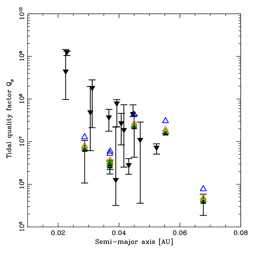
Figure 2.— Estimated tidal $Q$ factors for the case of slowly rotating stars ($\Omega_{*}/n<(\Omega_{*}/n)_{\rm crit}$). Upper/lower limits calculated from Eq. 6 are shown in black down/up triangles for planets with zero/non-zero eccentricities. Open triangles are the corresponding estimates from Eq. 1, which approach black ones as we take 2, 5, and 10 times the minimum stellar tidal $Q$s (blue, orange, and green triangles, respectively) obtained from Eq. 9.

Figure 2 shows the upper and lower limits for the planets’ $Q$ values as a function of semi-major axis for circular and eccentric orbits, respectively. Since the lower limits on $Q$ values for eccentric planets depend on $Q_{*}^{\prime}$, we take three different cases of $Q_{*}^{\prime}=2$, $5$, and $10\,Q_{*,{\rm min}}^{\prime}$ as examples. Note that, with this definition of $Q_{*}^{\prime}$, $Q_{\rm p}^{\prime}$ becomes independent of the stellar spin rate. Since circularization times are shorter for planets with smaller orbital radii, we tend to overestimate the maximum $Q$ values at the shortest-period end. All transiting planets appear within the range $10^{5}\lesssim Q_{\rm p}^{\prime}\lesssim 10^{9}$. The figure also shows that the high eccentricities of some planets (marked with upper triangles) can be explained by assuming relatively large ($Q_{\rm p}^{\prime}\gtrsim 10^{6}$) but reasonable ($Q_{\rm p}^{\prime}\lesssim 10^{9}$) tidal $Q$ values.

Although these estimated $Q$ values are larger than those of Jupiter or Neptune, they cannot be excluded. Recent theoretical studies of the excitation and dissipation of dynamical tides within rotating giant planets have shown that tidal $Q$ values fluctuate strongly depending on the tidal forcing frequency, and the effective $Q$’s could go up to $\sim 10^{9}$ depending on the spin rate and internal structure of the planet (e.g., presence/absence of a core, radiative envelope, or a density jump, see Ogilvie & Lin, 2004; Wu, 2005). According to these recent models, it appears possible that some planets maintain large eccentricities simply because of their larger $Q$ values.

3. Dynamical Perturbations

Candidate perturbation mechanisms that could excite and maintain planetary eccentricities include (1) tidal interaction with the central star (Dobbs-Dixon et al., 2004), (2) quadrupole or higher-order secular perturbation from an additional body, or (3) resonant interaction with another planet. Here we discuss the effects of these competing mechanisms against tidal eccentricity damping.

Tidal dissipation inside the central star can increase the planet eccentricity only when $\Omega_{*,{\rm rot}}>n$, or equivalently $de/dt>0$ in Eq. 1. For a synchronized planet ($\Omega_{p,{\rm rot}}\sim n$) with a small eccentricity ($e^{2}\ll 1$), we obtain $\Omega_{*,{\rm rot}}/n>18/11(1+7/18(Q_{*}^{\prime}/Q_{\rm p}^{\prime})(M_{*}/M_{\rm p})^{2}(R_{\rm p}/R_{*})^{5})$. For a Jupiter-like planet around a main-sequence star, this yields $\Omega_{*,{\rm rot}}>9.6n$ for $Q_{*}^{\prime}\sim Q_{\rm p}^{\prime}$. Since the rotation period for planet-hosting stars typically lies in the range 3 – 70 d, eccentricity excitation may occur for planets only if their orbital periods are within 29 – 673 d or longer. For a $10M_{\rm J}$ planet with radius $1R_{\rm J}$, we have $\Omega_{*,{\rm rot}}>1.7n$, which corresponds to an orbital period greater than 5.1 d. Therefore, this is unlikely to be responsible for the eccentricity of observed planets within $a\sim 0.06$–0.18 AU.

Another possibility is an undetected additional planet exciting the eccentricity of the detected planet. If there is a large mutual inclination angle ($i\gtrsim 40^{\circ}$) between the two planets, Kozai-type perturbations can become important (Kozai, 1962). Such highly non-coplanar orbits could result from planet–planet scattering after dissipation of the gaseous disk. Chatterjee et al. (2007); Nagasawa et al. (2008) have performed extensive numerical scattering experiments and showed that the final inclination of planets could be as high as $70^{\circ}$, with a median of 10 – $20^{\circ}$. If $i\lesssim 40^{\circ}$, octupole perturbations may still moderately excite the eccentricity of the close-in planet. The secular interaction timescale of a pair of planets with small mutual inclination can be derived from the classical Laplace-Lagrange theory (Brouwer & Clemence, 1961; Murray & Dermott, 1999).

For this secular perturbation from an additional planet to be causing the large eccentricity of the close-in planet, it must occur fast enough compared to other perturbations causing orbital precession. In particular, GR precession and tides are important effects that would compete against the perturbation from the additional body . For detailed discussions see Holman et al. (1997); Kiseleva et al. (1998).

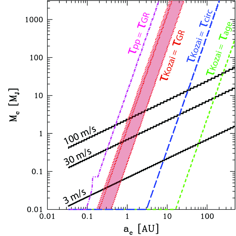
Figure 3.— Various secular eccentricity excitation timescales for the planet GJ 436 b caused by a hypothetical planetary (or stellar) companion GJ 436 c with mass $M_{\rm c}$ and semi-major axis $a_{\rm c}$. The solid black lines show the predicted radial velocity amplitudes caused by the undetected companion. The dot-dashed line shows the threshold right of which the secular interaction between planets with $i\lesssim 40$ deg is suppressed by GR precession, while the three red dotted lines are the similar thresholds for the Kozai mechanism with the assumed orbital eccentricity of the companion $e_{\rm c}=$ 0.01, 0.5, and 0.9 from left to right. We use $\tau_{\rm pp}$, $\tau_{\rm Kozai}$, and $\tau_{\rm GR}$ as in Takeda et al. (2008); Fabrycky & Tremaine (2007). Thresholds for $\tau_{\rm circ}$ and $\tau_{\rm age}$ are also shown for comparison.

Figure 3 illustrates the constraints on the mass and orbital radius of the hypothetical outer planet in the GJ 436 system. These are set by comparing the GR precession and secular timescales. Similar results are seen for other systems with eccentric close-in planets. Generally GR precession occurs faster than any other perturbation mechanism. In order to induce Kozai cycles in the inner planet (left of the dotted lines) while not causing radial-velocity amplitudes above the detection limit of $\sim 5\,{\rm m}\,{\rm s}^{-1}$ (below black lines), the mass upper limit of the hypothetical planet is $\sim 1M_{\rm Neptune}$. For near-coplanar systems even tighter constraints are placed on the properties of the secondary planet (left of the dot-dashed line).

However, one caveat is that our diagram only rules out the possibility of hypothetical bodies being currently responsible for the high eccentricity of GJ 436 b. Also, while Kozai-type perturbations are almost always suppressed by GR precession, eccentricity excitation through secular octupole perturbations may be occasionally enhanced by GR effects (Ford et al., 2000; Adams & Laughlin, 2006). For the case of the GJ 436 system, we have numerically tested the effect of a hypothetical secondary planet c on the eccentricity evolution of the inner planet b. We have found that, within the detectable radial-velocity limit $\lesssim 5\,m/s$, planet c cannot excite the eccentricity of planet b from 0.01 to the observed 0.15, even if its eccentricity is as high as 0.5. This result holds for other systems since they have even heavier planets. Therefore, we can safely exclude the possibility that these planets obtain their current high eccentricities through secular perturbation from an undetected outer planet with $\lesssim M_{\rm Neptune}$ if their orbits are initially near-circular.

Yet another possibility is a resonant perturbation from an undetected planet. Recently Ribas et al. (2008) suggested that the eccentricity of GJ 436 b might be caused by a mean-motion resonance (MMR) with an unseen super-Earth, but there is little observational support for this (e.g. Bean & Seifahrt, 2008). Also, the combined effects of GR precession and MMR are not fully understood yet. In any case, it is unlikely that such resonances are responsible for all the close-in eccentric planets, considering the small fraction of extrasolar multiple planets in MMR.

4. Summary

In this letter, we have investigated the origins of close-in planets on an eccentric orbit. We place constraints on the tidal Q factor of transiting planets by comparing the stellar age with the tidal circularization time, and find that $10^{5}\lesssim Q_{\rm p}^{\prime}\lesssim 10^{9}$, which agrees well with current theoretical estimates, can explain these eccentric planets. We also show that it is difficult to explain the high eccentricities of these planets by invoking a current interaction with an unseen second planet. Our results suggest that at least some of the close-in eccentric planets may be simply in the process of getting circularized.

This work was supported by NSF Grant AST-0507727.

Table 1Data are from http://exoplanet.eu/. Ages are computed using the stellar evolution database in Takeda et al. (2007), unless marked with $\ast$. Median values of the derived posterior age probability distribution functions are presented here, together with the 95% credible intervals in parenthesis.

Planet ID	$M_{\rm p}$ [$M_{J}$]	$R_{\rm p}$ [$R_{J}$]	$a$ [AU]	e	$M_{*}$ [$M_{\odot}$]	$R_{*}$ [$R_{\odot}$]	Age [Gyr]
OGLE-TR-56 b	1.29	1.3	0.0225	0	1.17	1.32	0.92 (0.20 –3.00)
OGLE-TR-113 b	1.32	1.09	0.0229	0	0.78	0.77	13.28 (11.00 – 13.92)
GJ 436 b $\ast$	0.072	0.38	0.02872	0.15	0.452	0.464	6.00 (1.00 – 10.00)
OGLE-TR-132 b	1.14	1.18	0.0306	0	1.26	1.34	0.96 (0.12 – 3.84)
HD 189733 b	1.15	1.156	0.0312	0	0.8	0.753	8.96 (1.04 – 13.72)
TrES-2 $\ast$	1.98	1.22	0.0367	0	0.98	1	5.10 (2.40 – 7.80)
WASP-14 b $\ast$	7.725	1.259	0.037	0.095	1.319	1.297	0.75 (0.5 – 1)
WASP-10 b $\ast$	3.06	1.29	0.0371	0.057	0.71	0.783	0.8 (0.6 – 1)
HAT-P-3 b $\ast$	0.599	0.89	0.03894	0	0.936	0.824	0.40 (0.10 – 6.90)
TrES-1	0.61	1.081	0.0393	0	0.87	0.82	11.40 (3.20 – 13.84)
HAT-P-5 b $\ast$	1.06	1.26	0.04075	0	1.16	1.167	2.60 (0.80 – 4.40)
OGLE-TR-10 b	0.63	1.26	0.04162	0	1.18	1.16	1.20 (0.16 – 4.64)
HD 149026 b $\ast$	0.36	0.71	0.0432	0	1.3	1.45	2.00 (1.20 – 2.80)
HAT-P-4 b $\ast$	0.68	1.27	0.0446	0	1.26	1.59	4.20 (3.60 – 6.80)
HD 209458 b	0.69	1.32	0.045	0.07	1.01	1.12	2.40 (0.48 – 4.60)
OGLE-TR-111 b	0.53	1.067	0.047	0	0.82	0.831	5.17 (0.17 – 13.41)
HAT-P-6 b $\ast$	1.057	1.33	0.05235	0	1.29	1.46	2.30 (1.60 – 2.80)
HAT-P-1 b $\ast$	0.524	1.36	0.0553	0.067	1.133	1.115	3.60
HAT-P-2 b $\ast$	8.64	0.952	0.0677	0.517	1.298	1.412	2.70 (1.30 – 4.10)

References

- Adams & Laughlin (2006) Adams, F. C. & Laughlin, G. 2006, ApJ, 649, 992
- Barnes (2001) Barnes, S. A. 2001, ApJ, 561, 1095
- Bean & Seifahrt (2008) Bean, J. L. & Seifahrt, A. 2008, ArXiv e-prints, 806
- Brouwer & Clemence (1961) Brouwer, D. & Clemence, G. M. 1961, Methods of celestial mechanics (New York: Academic Press, 1961)
- Carone & Pätzold (2007) Carone, L. & Pätzold, M. 2007, P&SS, 55, 643
- Chatterjee et al. (2007) Chatterjee, S., Ford, E. B., Matsumura, S., & Rasio, F. A. 2007, ArXiv Astrophysics e-prints
- Dobbs-Dixon et al. (2004) Dobbs-Dixon, I., Lin, D. N. C., & Mardling, R. A. 2004, ApJ, 610, 464
- Eggleton et al. (1998) Eggleton, P. P., Kiseleva, L. G., & Hut, P. 1998, ApJ, 499, 853
- Faber et al. (2005) Faber, J. A., Rasio, F. A., & Willems, B. 2005, Icarus, 175, 248
- Fabrycky & Tremaine (2007) Fabrycky, D. & Tremaine, S. 2007, ApJ, 669, 1298
- Ford et al. (2000) Ford, E. B., Kozinsky, B., & Rasio, F. A. 2000, ApJ, 535, 385
- Ford & Rasio (2006) Ford, E. B. & Rasio, F. A. 2006, ApJL, 638, L45
- Goldreich & Soter (1966) Goldreich, P. & Soter, S. 1966, Icarus, 5, 375
- Hebrard et al. (2008) Hebrard, G., et al. 2008, ArXiv e-prints, 806
- Holman et al. (1997) Holman, M., Touma, J., & Tremaine, S. 1997, Nature, 386, 254
- Hut (1981) Hut, P. 1981, A&A, 99, 126
- Kiseleva et al. (1998) Kiseleva, L. G., Eggleton, P. P., & Mikkola, S. 1998, MNRAS, 300, 292
- Kozai (1962) Kozai, Y. 1962, AJ, 67, 591
- Marcy et al. (1997) Marcy, G. W., Butler, R. P., Williams, E., Bildsten, L., Graham, J. R., Ghez, A. M., & Jernigan, J. G. 1997, ApJ, 481, 926
- Mardling & Lin (2002) Mardling, R. A. & Lin, D. N. C. 2002, ApJ, 573, 829
- Murray & Dermott (1999) Murray, C. D. & Dermott, S. F. 1999, Solar system dynamics (Solar system dynamics by Murray, C. D., 1999)
- Nagasawa et al. (2008) Nagasawa, M., Ida, S., & Bessho, T. 2008, ArXiv e-prints, 801
- Narita et al. (2007) Narita, N., Sato, B., Ohshima, O., & Winn, J. N. 2007, ArXiv e-prints, 712
- Ogilvie & Lin (2004) Ogilvie, G. I. & Lin, D. N. C. 2004, ApJ, 610, 477
- Queloz et al. (2000) Queloz, D., et al. 2000, A&A, 359, L13
- Rasio et al. (1996) Rasio, F. A., Tout, C. A., Lubow, S. H., & Livio, M. 1996, ApJ, 470, 1187
- Ribas et al. (2008) Ribas, I., Font-Ribera, A., & Beaulieu, J.-P. 2008, ArXiv e-prints, 801
- Sterne (1939) Sterne, T. E. 1939, MNRAS, 99, 451
- Takeda et al. (2007) Takeda, G., Ford, E. B., Sills, A., Rasio, F. A., Fischer, D. A., & Valenti, J. A. 2007, ApJS, 168, 297
- Takeda et al. (2008) Takeda, G., Kita, R., & Rasio, F. A. 2008, ArXiv e-prints, 802
- Winn et al. (2005) Winn, J. N., et al. 2005, ApJ, 631, 1215
- Wu (2005) Wu, Y. 2005, ApJ, 635, 688
- Yoder & Peale (1981) Yoder, C. F. & Peale, S. J. 1981, Icarus, 47, 1
- Zhang & Hamilton (2008) Zhang, K. & Hamilton, D. P. 2008, Icarus, 193, 267