The entanglement in one-dimensional random XY spin chain with Dzyaloshinskii-Moriya interaction

Abstract

The impurities of exchange couplings, external magnetic fields and Dzyaloshinskii–Moriya (DM) interaction considered as Gaussian distribution, the entanglement in one-dimensional random $XY$ spin systems is investigated by the method of solving the different spin-spin correlation functions and the average magnetization per spin. The entanglement dynamics at central locations of ferromagnetic and antiferromagnetic chains have been studied by varying the three impurities and the strength of DM interaction. (i) For ferromagnetic spin chain, the weak DM interaction can improve the amount of entanglement to a large value, and the impurities have the opposite effect on the entanglement below and above critical DM interaction. (ii) For antiferromagnetic spin chain, DM interaction can enhance the entanglement to a steady value. Our results imply that DM interaction strength, the impurity and exchange couplings (or magnetic field) play competing roles in enhancing quantum entanglement.

I Introduction

Entanglement is not only important in the quantum information processing (QIP), such as quantum teleportation,^[1] dense coding,^[2] quantum secret sharing,^[3] quantum computation,^[4] but also relevant to quantum phase transitions^[5] in condensed matter physics. In order to realize quantum information process, great effort has been devoted to studying and characterizing the entanglement in cavity QED.^[6-8] Now, much attention has been paid to the entanglement in spin systems, such as the Ising model^[9] and all the kinds of Heisenberg XY XXZ XYZ models.^[10-13] However; as far as we know, most discussions mentioned above merely focused on the models with spin exchange couplings, while Dzyaloshinskii–Moriya interaction has seldom been taken into account. The antisymmetric DM interaction, introduced by Dzyaloshinskii and Moriya, is a combination of superexchange and spin-orbital interactions. In fact, some one-dimensional and two-dimensional spin models have manifested such interactions.^[14,15] Therefore, it is worthwhile including DM interaction in the studies of spin chain entanglement.
Impurities necessarily exist in real materials and their effects are more pronounced in condensed matter physics. Thus, it is important to study the effects of impurities in view of the possible realizations of one-dimensional ferromagnetic and antiferromagnetic chains. In the previous researches, the impurity effects on the quantum entanglement have been studied in a three-spin system^[16,17] and a large spin systems under zero temperature.^[18] However, in these works, they have just studied single impurity.
Recently, Huang et al.,^[19] Osenda et al.^[20] and we^[21] have demonstrated that for a class of one-dimensional magnetic systems, entanglement can be controlled and tuned by introducing impurities into the systems. For the pure case, Osterloh et al.^[22] examined the entanglement between two spins of position $i$ and $j$ in the spin chain as the system goes through quantum phase transition. They demonstrated that entanglement shows scaling behaviour in the vicinity of the transition point. For a two-qubit spin chain with DM interaction, researchers^[23,24] have considered thermal entanglement and teleportation. For a particular spin system the allowed components of the DM interaction are determined by the corrections to the energy symmetry of the spin complex. Since the DM terms break spin-spin rotational symmetry, we need to calculate how spin exchange couplings and DM interaction have effect on the entanglement and phase transition point. It is an interesting quantum phenomenon that the entanglement shares many features with quantum phase transition (QPT), QPT is a critical change in the properties of the ground state of a many body system due to modifications in the interactions among its constituents. The associated level crossings lead to the presence of non-analyticities in the energy spectrum. Therefore, the knowledge about the entanglement, the non-local correlation in quantum systems, is considered as the key to understand QPT. That is the purpose and motivation of the present work to investigate the behaviour of entanglement at and around the quantum critical point in one-dimensional $XY$ spin system with DM interaction, which can display a variety of interesting physical phenomena providing new insight in two-site entanglement and the related QPT as well under the effect of the impurities of exchange couplings, external magnetic fields and DM interaction.
We consider Heisenberg $XY$ model of $N$ spin-$\frac{1}{2}$ particles with nearest-neighbour interactions. In the presence of impurities and DM interaction,^[25] one-dimensional Hamiltonian is given by^[19]

$$H=-\frac{1+\gamma}{2}\sum_{i=1}^{N}J_{i,i+1}\sigma_{i}^{x}\sigma_{i+1}^{x}-\frac{1-\gamma}{2}\times\sum_{i=1}^{N}J_{i,i+1}$$

$$\times\sigma_{i}^{y}\sigma_{i+1}^{y}-\sum_{i=1}^{N}h_{i}\sigma_{i}^{z}-\frac{1}{2}\sum_{i=1}^{N}\vec{D}_{i,i+1}\cdot(\vec{\sigma}_{i}\times\vec{\sigma}_{i+1})$$ (1)

where $J_{i,i+1}$ and $D_{i,i+1}$ are exchange interaction and DM interaction along $z$-direction between sites $i$ and $i+1$ respectively, $h_{i}$ is the strength of external magnetic field on site $i$, $\sigma^{x,y,z}$ are the Pauli matrices, $\gamma$ is the degree of anisotropy and $N$ is the number of sites. For all the interval $0<\gamma\leq 1$ and $N=\infty$, they undergo a quantum phase transition at the critical value $\lambda_{c}=1$. The periodic boundary conditions satisfy $\sigma_{N+1}^{x}=\sigma_{1}^{x},\sigma_{N+1}^{y}=\sigma_{1}^{y},\sigma_{N+1}^{z}=\sigma_{1}^{z}$. Let us define the raising and lowing operators $a_{i}^{+}$, $a_{i}^{-}$ and introduce Fermi operators $c_{j}^{+}$ and $c_{j}$,^[26] the Hamiltonian has the form

$$H=-\sum_{i=1}^{N}[((J_{i,i+1}+iD_{i,i+1})c_{i}^{+}c_{i+1}+h.c)+$$

$$(J_{i,i+1}\gamma c_{i}^{+}c_{i+1}^{+}+h.c)]-2\sum_{i=1}^{N}h_{i}(c_{i}^{+}c_{i}-\frac{1}{2})$$ (2)

In this study, the exchange interaction has the form $J_{i,i+1}=J(1+\alpha_{i,i+1})$, where $\alpha$ introduces the impurity in a Gaussian form centered at $\dfrac{N+1}{2}$ with strength or height $\zeta$, $\alpha_{i,i+1}=\zeta\exp\Big{(}-\epsilon\Big{(}i-\dfrac{N+1}{2}\Big{)}\Big{)}$, $\epsilon$ is the value of the width of the distribution. For $J<0$, the spin chain is antiferromagnetic; for $J>0$, the spin chain is ferromagnetic. The external magnetic field and Dzyaloshinskii–Moriya interaction take the form $h_{i}=h(1+\beta_{i})$ and $D_{i,i+1}=D(1+\eta_{i,i+1})\exp\Big{(}\dfrac{\pi}{2}i\Big{)}$, where $\beta_{i}=\xi\exp\Big{(}-\epsilon\Big{(}i-\dfrac{N+1}{2}\Big{)}\Big{)}$, $\eta_{i,i+1}=\kappa\exp\Big{(}-\epsilon\Big{(}i-\dfrac{N+1}{2}\Big{)}\Big{)}$. When $\alpha=\beta=\eta=0$, we recover the pure case; when $\eta=0$, we recover the case described in Ref. [19]. For the distributions of exchange interaction impurity, Dzyaloshinskii–Moriya interaction impurity and the magnetic field impurity, we fix the value of width of the distribution at $\epsilon=0.1$ in all the calculations. As the center $\Big{(}\dfrac{N+1}{2}\Big{)}$ and the width ($\epsilon$) of the Gaussian distribution are fixed, we can obtain different impurities $\alpha,\,\beta,\,\eta$ of the Gaussian distributions only by changing strengths or heights $\zeta,\,\xi,\,\kappa$. By introducing the dimensionless parameter $\lambda=J/2h$, the symmetrical matrix $A$ and the antisymmetrical $B$, the Hamiltonian becomes

$$H=\sum_{i,j=1}^{N}[c_{i}^{+}A_{i,j}c_{j}+\frac{1}{2}(c_{i}^{+}B_{i,j}c_{j}^{+}+h.c)]$$ (3)

The above Hamiltonian can be diagonalized by making linear transformation of the fermionic operators $\eta_{k}=\sum_{i=1}^{N}g_{ki}c_{i}+h_{ki}c_{i}^{+},\eta_{k}^{+}=\sum_{i=1}^{N}g_{ki}c_{i}^{+}+h_{ki}c_{i},$ then the Hamiltonian becomes

$$H=\sum_{k=1}^{N}\Lambda_{k}\eta_{k}^{+}\eta_{k}+const,$$ (4)

two coupled matrix equations satisfy $\phi_{k}(A-B)=\Lambda_{k}\psi_{k},$ $\psi_{k}(A+B)=\Lambda_{k}\phi_{k},$ where the components of the two column vectors $\phi_{ki},\psi_{ki}$ are given by $\phi_{ki}=g_{ki}+h_{ki},\psi_{ki}=g_{ki}-h_{ki}.$ Finally, the ground state of the system $|\psi_{0}\rangle$ can be written as $\eta_{k}|\psi_{0}|=0$.

Using Wick’s theorem,^[27] spin-spin correlation functions for the ground state and the average magnetization per spin can be expressed as
$S_{lm}^{x}=\frac{1}{4}\left(\begin{array}[]{cccc}G_{l,l+1}&G_{l,l+2}&\cdots&G_{l,m}\\ \vdots&\vdots&\ddots&\vdots\\ G_{m-1,l+1}&G_{m-1,l+1}&\cdots&G_{m-1,m}\end{array}\right)$,
$S_{lm}^{y}=\frac{1}{4}\left(\begin{array}[]{cccc}G_{l+1,l}&G_{l+1,l+1}&\cdots&G_{l+1,m-1}\\ \vdots&\vdots&\ddots&\vdots\\ G_{m,l}&G_{m,l+1}&\cdots&G_{m,m-1}\end{array}\right)$,
$S_{lm}^{z}=\frac{1}{4}(G_{l,l}G_{m,m}-G_{m,l}G_{l,m}),M_{i}^{z}=\frac{1}{2}G_{i,i}$
where $G_{i,j}=-\sum_{k}^{N}\psi_{ki}\phi_{kj}$ Next, we give the expression of concurrence that quantifies the amount of entanglement between two qubits.

For a system described by the density matrix $\rho$, the concurrence $C$ reads^[28]

$$C(\rho)=\max(0,\lambda_{1}-\lambda_{2}-\lambda_{3}-\lambda_{4})$$ (5)

where $\lambda_{1}$, $\lambda_{2}$, $\lambda_{3}$, and $\lambda_{4}$ are the eigenvalues (with $\lambda_{1}$ being the largest one) of the spin-flipped density operator $R$, which is defined by $R=\sqrt{\sqrt{\rho}\tilde{\rho}\sqrt{\rho}}$, where $\tilde{\rho}=(\sigma_{y}\otimes\sigma_{y})\rho^{*}(\sigma_{y}\otimes\sigma_{y})$; $\tilde{\rho}$ denotes the complex conjugate of $\rho$; $\sigma_{y}$ is the usual Pauli matrix. Using the operator expansion for the density matrix and the symmetries of the Hamiltonian,^[29] in the basis states $\{|\uparrow\uparrow\rangle,\,|\uparrow\downarrow\rangle,\,|\downarrow\uparrow\rangle,|\downarrow\downarrow\rangle\}$, $\rho$ has the general form. We can express all the matrix elements in the density matrix in terms of different spin-spin correlation functions.
In this study, we focus our discussion on the transverse Ising model with $\gamma=1$. We examine the dynamics of entanglement in varying the impurities of exchange couplings, external magnetic fields and Dzyaloshinskii–Moriya interaction. First, we examine the change of the entanglement for the nearest-neighbouring concurrence $C(i,i+1)$ for different values of the impurity as the parameter $\lambda$ varies. Figure 1 depicts the nearest-neighbouring concurrence $C(49,50)$ as a function of the reduced coupling constant $\lambda$ at different values of the exchange couplings impurity $\zeta$ and external magnetic fields impurity $\xi$ with the system size $N=99$. Figure 1(a) shows the change of concurrence $C(49,50)$ as a function of $\lambda$ for different values of exchange couplings impurity with $D=0$, i.e. in the absence of DM interaction. For the case of $\lambda>0$, we can see that the concurrence increases and arrives at a maximum close to the critical point $\lambda_{c}$, while it is close to zero above $\lambda_{c}$. As $\zeta$ increases the concurrence tends to increase faster, and $\lambda_{m}$, where concurrence approaches a maximum, shifts to left very rapidly. This is consistent with the result reported in Refs. [19,21] (Fig.1). A similar behaviour can be seen for the case of $\lambda<0$, that is to say, the entanglement has equal value for ferromagnetic and antiferromagnetic chains with the same $|\lambda|$. The effect of the external magnetic field $\xi$ in the Gaussian distribution is also shown in Fig.1(b). However, different from the effect of the exchange couplings, the concurrence increases slowly and tends to moving to infinity by increasing the value of the parameter $\xi$. This is also consistent with the result in Refs.[19,21] (Fig.1). In Figs.1(c) and 1(d), taking DM interaction into account, we give a plot of the concurrence against exchange couplings impurity and external magnetic field impurity with $D=0.5|J|$. As $\zeta$ increases, the concurrence increases slowly and the peak value decreases, which can be seen in Fig.1(c), different from the result in Fig.1(a) for ferromagnetic spin chain. Moreover, some interesting physical phenomena occur for the antiferromagnetic chain, for example, the concurrence decreases to zero at the critical point ($\lambda_{0}$) and increases from zero to a finite steady value across the transition point. Therefore, we can further understand the relation between the entanglement and quantum transition. In Fig.1(d), the numerical calculations show that the steady concurrence decreases with the increase of $\xi$ for the antiferromagnetic chain, which indicates that the behaviour is very different from those in Fig.1(b). Now weexplain why the curves of concurrence have some maximum or minimum at some special values of the DM interactions and external magnetic fields. As $[\partial C(49,50)/\partial\lambda]_{\lambda_{c}}$ diverges, the maximal or minimal entanglement will not occur at the critical point but in the vicinity of the transition point ($[\partial C(49,50)/\partial\lambda]_{\lambda_{m}}=0,$ $[\partial^{2}C(49,50)/\partial^{2}\lambda]_{\lambda_{m}}<0$ or $[\partial^{2}C(49,50)/\partial^{2}\lambda]_{\lambda_{m}}>0$). In our model, when $D=0$, quantum transition point $\lambda_{c}=\dfrac{1+\beta_{i,i+1}}{1+\alpha_{i,i+1}}$, from the above expression, we can know the transition point shifts and is affected by the impurities of exchange couplings and external magnetic fields. For the entanglement length (or the correlation length), the position of the related maximal and minimal concurrence will shift in the same way. However, DM interactions lead to different coefficients in the first two parts of Eq.(2), so the critical point $\lambda_{c}$ occurs between the two ones $\Big{(}\dfrac{1+\beta_{i,i+1}}{1+\alpha_{i,i+1}},\dfrac{1+\beta_{i,i+1}}{1+\alpha_{i,i+1}-\frac{D}{J}(1+\eta_{i,i+1})}\Big{)}$. For the case of $J<0$, there exist two critical points. Of course, we can figure out exact critical value and maximum or minimum of the concurrence through solving the first order and second order derivative of the entanglement respectively.
From Fig.1, we can see that DM interaction plays an important role in enhancing entanglement, so it is necessary to study the effect of DM interaction on the entanglement. In Fig.2, we show the results of the nearest-neighbouring concurrence as a function of the parameter $\lambda$ for DM interaction impurity at different strengths of DM interaction $D$. We can easily find that the competing roles played by DM interaction impurity $\kappa$, strength $D$ and exchange couplings $J$ (the external magnetic field is fixed) in enhancing quantum entanglement will exist in spin chain. The competing effect leads to shift of the critical point and the entanglement. The results show that when the absolute value of $\lambda$ is below $\lambda_{c}$, the concurrence only increases with $|\lambda|$, DM interaction impurities will have no effect on the entanglement once strength is fixed, i.e. exchange couplings is predominant in the competing role. The effect of weak DM interaction strength $D=0.1|J|$ is shown in Fig.2(a). Contrast to the exchange couplings impurity, DM interaction impurity can enhance the entanglement, the concurrence increases and tends to move to infinity($>0$) by increasing the value of the parameter $\kappa$. It is interesting to find that the entanglement peak and steady value between the nearest neighbours with $D=0.5|J|$ increase to a value larger than those in Fig. 2(a). With the increasing $D$, in Fig.2(c), the concurrence decreases as $\kappa$ increases. We can imagine that there must be a critical DM strength ($D_{c}$), below $D_{c}$, impurity enhances entanglement, while above $D_{c}$, impurity shrinks entanglement. In other words, at some special values of the DM interactions, the entanglement varies at different critical vicinities, which is similar to the analysis in Fig.1. The comparison among the different curve in Fig.2(d) shows that the concurrence decreases rapidly above $\lambda_{c}$ by increasing the value of the parameter $\kappa$, which is different from the results obtained from Figs. 2(a) and 2(b). That is to say, the strong $D$ is not helpful to keeping the better entanglement for Gaussian distribution.
The effect of DM strength is demonstrated in Fig.3 by the evolutions of the concurrence. Figure 3(a) corresponds to the case of $\kappa=0$, the nearest-neighbouring concurrence increases with the increase of $D$, a critical point occurs with small DM interaction strength and the peak of the maximal entanglement becomes larger. It is the DM interaction that leads to considerable different evolutions of the entanglement, hence the entanglement is rather sensitive to any small change with the DM interaction. Thus, by adjusting DM interaction one can obtain a strong entanglement. Similar behaviours to those in Figs.2(c)and 2(d) are shown in Figs.3(c) and 3(d), we can see that DM interaction strength is not certain to enhance the entanglement, and the entanglement tends to be reduced in the presence of strong DM interaction at $\kappa=1.0$. The results we have obtained here are also consistent with those in Fig.2.
According to finite-size scaling analysis, the two-site entanglement is considered as a function of the system size (including the thermodynamic limit) and the distance $|\lambda-\lambda_{c}|$ from the critical point. The entanglement can approximately collapse to a single curve for different system sizes ranging from 41 up to 401, thus all key ingredients of the finite-size scaling are present in the concurrence. The first order derivative around the critical point becomes sharper (the peak position $\lambda_{\min}$ approaches the critical point $\lambda_{c}$) as the system size increases, and is expected to be divergent in an infinite system ($\partial C/\partial\lambda=A_{1}\ln|\lambda-\lambda_{c}|+{\rm const}$). Though there is no divergence when $N$ is finite, the anomalies are obvious. Its value diverges logarithmically with the increasing system size as $\partial C/\partial\lambda=A_{2}\ln N+{\rm const}$. Thus, we can see that the QPT of the system is reflected by the behaviour of the concurrence and its $\lambda$ derivative and finite size scaling is fulfilled over a very broad range of values of $N$, which are of interest in quantum information.
In summary, from the above analysis, it is clearly noted that the three different impurities and DM interaction strength, which play the competing roles in enhancing quantum entanglement, have a notable influence on the nearest-neighbouring concurrence in the one-dimensional $s=\dfrac{1}{2}$ random $XY$ spin system. The nearest-neighbouring concurrence exhibits some interesting phenomena. For an antiferromagnetic spin chain, there is a critical point where the entanglement is zero. DM interaction is predominant in the competing role and can enhance the entanglement to a steady value. For a ferromagnetic spin chain, the weak DM interaction can improve the amount of entanglement to a large value. However, under condition of strong DM interaction, there is a critical point $D_{c}$ where the impurities have the opposite effect on the entanglement below and above $D_{c}$. Thus we can employ DM interaction strength as well as three different impurities to realize quantum entanglement control. For the case of $\gamma\neq 1$ (XY model) or the next nearest-neighbouring concurrence related QPT, we will present further reports in the future.

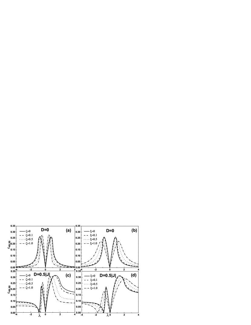
Figure 1: The nearest neighbour concurrence $C(49,50)$ for the impurities $\zeta$ and the impurities $\xi$ as a function of the reduced coupling constant $\lambda$ with $N=99$, $\gamma=1$, $\kappa=0$.

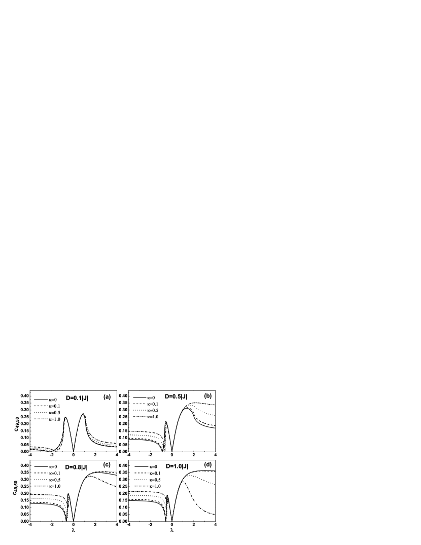
Figure 2: The nearest neighbour concurrence $C(49,50)$ as a function of the parameter $\lambda$ for the DM interaction impurities $\kappa$ with $N=99$, $\gamma=1$, $\zeta=\xi=0$.

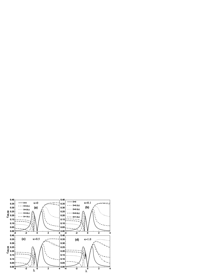
Figure 3: The nearest neighbour concurrence $C(49,50)$ as a function of the parameter $\lambda$ for the DM interaction strength $D$ with $N=99$, $\gamma=1$, $\zeta=\xi=0$.

References

-
(1)
Bennett C H, Brassard G, Cr peau C, Jozsa R, Peres A, and Wootters W K, 1993 Phys. Rev. Lett. 70 1895.
Shan C J, Man Z X, Xia Y J, Liu T K. 2007 I. J. Quantum Information, 5 359. - (2) Cheng W W, Huang Y X, Liu T K and Li H, 2007 Chin. Phys. 16 38.
- (3) Shan C J, Man Z X, Xia Y J, Liu T K. 2007 I. J. Quantum Information, 5 335.
- (4) Grover L 1998 Phys. Rev. Lett. 80 4329.
- (5) Gu S J,Tian G S, Lin H Q 2007 Chin. Phys. Lett. 24 2737.
- (6) Shan C J, Xia Y J 2006 Acta. Phys. Sin. 55 1585.(in Chinese)
- (7) Liu T K, 2007 Chin. Phys. 16 3396.
- (8) Lu D M and Zheng S B, 2007 Chin. Phys. Lett. 24 596.
- (9) Pang C Y and Li Y L, 2006 Chin. Phys. Lett. 23 3145.
- (10) Zhai X Y and Tong P Q, 2007 Chin. Phys. Lett. 24 2475.
- (11) Wu Y, Machta J, 2005 Phys. Rev. Lett. 95 137208.
- (12) Wang X G 2001 Phys. Rev. A 64 012313.
- (13) Zhang G F and Li S S, 2005 Phys. Rev. A 72 034302.
- (14) Zhao J Z, Wang X Q, Xiang T, Su Z B, Yu L, 2003 Phys. Rev. Lett. 90 2072041.
- (15) Chutia S, Friesen M, and Joynt R, 2006 Phys. Rev. B 73 241304.
- (16) Fu H C,Solomon A I, Wang X G, 2002 J. Phys. A 35 4293. Li S B, Xu J B, 2005 Phys. Lett. A 334 109.
- (17) Cheng W W, Huang Y X, Liu T K and Li H, 2007 Physica E 39 150.
- (18) Xin R, Song Z, Sun C P, 2005 Phys. Lett. A 342 30.
- (19) Huang Z, Osenda O, Kais S, 2004 Phys. Lett. A 322 137.
- (20) Osenda O, Huang Z, Kais S, 2003 Phys. Rev. A 67 062321.
- (21) Shan C J, Cheng W W, Liu T K, Huang Y X and Li H, 2008 Chin. Phys. 17 (in press)
- (22) Osterloh A, Amico L, Falci G, and Fazio R, 2002 Nature(London) 416 608.
- (23) Zhang G F, 2007 Phys. Rev. A 75 034304
- (24) Gurkan Z N, Pashaev O K 2007 arxiv: 0705.0679v1
- (25) Dzyaloshinsky I, Thermodynamic A 1958 J. Phys. Chem. Solids 4 241. Moriya T 1960 Phys. Rev. Lett. 4 228
- (26) Lieb E, Schultz T, Mattis D, 1961 Ann. Phys. 60 407.
- (27) Wick G C, 1950 Phys. Rev. 80 268.
- (28) Wooters W K, 1998 Phys. Rev. Lett. 80 2245.
- (29) Osborne T J, Nielsen M A, 2002 Phys. Rev. A 66 032110.