Bi-stability in voltage-biased NISIN structures

Abstract

As a generic example of a voltage-driven superconducting structure we study a short superconductor connected to normal leads by means of low transparency tunnel junctions, with a voltage bias $V$ between the leads. The superconducting order parameter $\Delta$ is to be determined self-consistently. We study the stationary states of the system as well as the dynamics after a perturbation. We find a region in parameter space where there are two stable stationary states at a given voltage. These bi-stable states are distinguished by distinct values of the superconducting order parameter $\Delta$ and of the current between the leads. We have evaluated (1) the multi-valued superconducting order parameter $\Delta$ at given $V$; (2) the current between the leads at a given V; and (3) the critical voltage at which superconductivity in the island ceases. With regards to dynamics, we find numerical evidence that the stationary states are stable and that no complicated non-stationary regime can be induced by changing the voltage. This result is somewhat unexpected and by no means trivial, given the fact that the system is driven out of equilibrium. The response to a change in the voltage is always gradual, even in the regime where changing the interaction strength induces rapid anharmonic oscillations of the order parameter.

I Introduction

Electron transport devices combining superconducting (S), insulating (I) and normal metal (N) elements are known as superconducting hetero-structures. Often such hetero-structures are more than the sum of their parts.Lam98 ; Bee95 Phenomena that are not present in bulk S, I or N systems appear when a device contains junction between these components. The following examples are well known: (1) The conductance of a high transparency NS junction does not equal the conductance of the normal metal on its own, as one might naively expect. If the normal metal is free of impurities, the conductance is higher than that of the normal metal.Blo82 This surprising effect is due to a process known as Andreev reflection.And64 During Andreev reflection at an NS interface, an electron impinging on the interface from the N side is reflected back as a hole, while a Cooper pair propagates away from the interface on the S side. (2) In Josephson junctions, the simplest of which is perhaps the SIS hetero-structure,Jos62 a DC current can flow at zero bias voltage. This happens when the superconducting phase difference across the junction is non-zero.Tin96

The above examples can be understood in terms of equilibrium properties of the hetero-structure. When a superconducting device is perturbed outside equilibrium, yet more interesting effects can occur,Kopnin for instance, oscillations under stationary non-equilibrium conditions. An elementary example: if a Josephson junction is biased with a DC (i.e. fixed) voltage, an AC (i.e. oscillating) current flows through the junction.Tin96 Another example of the kind has been investigated in the context of cold Fermi gases in optical traps. In these systems, the interaction between atoms can be tuned and changed by means of a so-called Feshbach resonance. If the interaction is attractive, the gas forms a BCS-condensate. Recent studiesBar06 ; Yuz05 have considered what happens if the value of the attractive pairing interaction is changed abruptly. It was discovered that, depending on the ratio between the initial and final values of the interaction strength, the condensate order parameter can perform anharmonic oscillations that do not decay in time.

The initial motivation for the research presented in this paper came form the study of Keizer et al.,Kei06 where the authors investigated the suppression of the superconducting order parameter by a voltage applied to a superconducting wire. It was assumed that $\Delta$ remains stationary. However, this assumption does not seem well-justified: the stationary voltage could induce periodic oscillations of $|\Delta|$ or even richer chaotic dynamics. Thus prompted, we wanted to address the validity of this assumption for a decidedly simpler NISIN structure, namely a short superconductor connected to normal leads by means of tunnel junctions. The structure is biased with a voltage $V$.

We require that (1) the dominant energy relaxation mechanism in the superconductor is the tunneling of electrons to the leads, and (2) spatial variations of the superconducting order parameter inside the superconductor are negligible. To meet the first requirement, the superconductor must have dimensions smaller than the inelastic scattering length of quasi-particles. This is not an unrealistic requirement given current experimental techniques. To meet the second requirement, the superconductor should firstly contain impurities or have an irregular shape, so that the electron wave-functions of the isolated island are isotropic on the scale of the superconducting coherence length.deG66 Secondly, the tunnel junctions connecting it to the leads should have a bigger normal-state resistance than that of the superconductor proper. In this case, opening up the system by connecting leads does not re-introduce spatial anisotropy of wave-functions inside the island.

The study of NISIN structures has a long history.Giaver ; Hidaku Our study complements several previous studies.Kei06 ; San01 ; Mar95 These dealt with quasi-one-dimensional superconducting wires between normal leads. Setups where either the superconductor was impurity-free or the transparency of the NS interfaces were high were considered. For these setups, spatial variations of the order parameter, specifically the spatial gradient of the superconducting phase, can be large. Including these spatial variations in the description of the superconductor significantly complicates matters. Hence these studies focused on numerical calculations and assumed that the superconducting order-parameter and all other quantities of interest were stationary. It should also be mentioned that asymmetric couplings, where the superconductor is coupled more strongly to one lead than the other, did not receive detailed analysis. The only asymmetric setup considered consisted of one interface with tunable transparency and the other perfectly transparent.Mar95 One of the main conclusions of these studies is that, if the bias voltage is large enough, the system switches to the normal state. Some evidence for a bi-stable region where, depending on the history of the system, either the superconducting or the normal state can occur at a given voltage, was reported.Kei06

The absence of spatial variations in the system we study allows us to perform analytical calculations, provided we assume stationarity. Results are obtained for an arbitrary ratio of the coupling strengths to the leads. We derive transcendental equations relating the superconducting order parameter to the bias voltage, and derive an explicit formula for the current between the leads. As mentioned, the assumption of stationarity is however not a priori justified. As was seen in the examples mentioned at the beginning of this introduction, non-equilibrium conditions in superconductors often go hand in hand with non-stationary behavior of observable quantities. Indeed, the NISIN junction that we study is a non-linear system subjected to a driving force (and to damping). Non-linearity here means that the dynamical equations for one-particle Green functions are not linear in the Green functions. This is due to the existence of a non-zero superconducting order parameter. The driving force is provided by the voltage (and the damping by tunneling of electrons from the island into the leads). Non-linear driven systems (think of the nonlinear pendulum) often have chaotic dynamics. The assumption of stationarity would miss this. We therefore supplement our analytical calculation with numerical calculations that study the dynamics in real time.

Our main results are the following: The stationary states that we found analytically are stable. Furthermore, there is a parameter region where two different stationary states are stable at the same voltage. (This is the “bi-stability” of the title.) For a symmetric coupling to the source and drain leads, one of the two states is superconducting (characterized by a non-zero order parameter) and the other is normal. Since we are in the regime of high tunnel barriers, at a given voltage, the superconducting island allows less current to flow between the leads than the island in the normal state.Blo82 This current is a directly measurable quantity and allows one to distinguish between superconducting and normal states. For some asymmetric couplings however, both the stable states are superconducting. We have calculated the current that flows between the leads at a given voltage, and at arbitrary asymmetry of the coupling to the two leads. We find that the value of the current also allows one to distinguish between different stable superconducting states at a given voltage.

The time-dependent calculations revealed that once the bias voltage becomes constant in time, the system always relaxes into one of the stationary states. Non-stationary behavior of physical quantities always decays in time, unlike in the case of a DC-biased Josephson junction. (Despite it being a non-linear system, a superconductor driven by a voltage is therefore fundamentally different from a nonlinear pendulum driven by an external force.) If the bias voltage is changed slowly, an initial stationary state evolves adiabatically. By changing the voltage slowly we have observed the expected hysteresis associated with the existence of two stable states at some voltages.

The rest of the paper is structured as follows. In Sec. II we specify the model to be studied, and present the equations that determine its state. In Sec. III we solve these equations analytically, assuming that the system is in a stationary state. We analyze the stationary stationary states we find and calculate the $I$-$V$ characteristic of the system. In Sec. IV we establish that the stationary states are the only stable states of the DC-biased system. We do so by studying the dynamics of the system after a perturbation. In Sec. V we summarize our main results.

II Model

As stated in the introduction, we consider a superconducting island connected to two normal leads by means of low transparency tunnel barriers. The superconducting order parameter is taken to be spatially isotropic inside the island. The physical requirements for this condition to hold have already been discussed in the introduction. We assume that the dominant energy relaxation mechanism for the superconductor is tunneling of electrons to the leads. For given barrier transparencies, this restricts the size of the superconductor to less than the inelastic scattering length of quasi-particles inside the superconductor.

Our analysis of the system is based on the Keldysh Green function technique.Kel64 ; Ram86 ; Brink03 We start our discussion of the equations governing the system by defining the necessary Green functions.

II.1 Definition of Green functions

The Green functions are expectation values of products of the Heisenberg operators $a_{m\pm}^{\dagger}(t)$ and $a_{m\pm}(t)$ that create and annihilate electrons in levels of the isolated island. Here $m$ labels single particle levels. The $\pm$ index accounts for Kramer’s degeneracy. As we are dealing with a problem involving superconductivity, all Green functions are $2\times 2$ matrices in Nambu space. It is useful to define Nambu space matrices $\eta_{j}$, $j=0,\ldots,3$ such that $\eta_{0}$ is the identity matrix and $\eta_{1}$, $\eta_{2}$ and $\eta_{3}$ are the standard Pauli matrices. We also define matrices $\eta_{\pm}=(\eta_{1}\pm i\eta_{2})/2$.

The retarded ($R$), Keldysh ($K$) and advanced ($A$) Green functions of each level are defined asNote1

$$R_{m}(t,t^{\prime}) = -i\eta_{3}\left<\left(\begin{array}[]{rr}\{a_{m+}(t),a_{m+}^{\dagger}(t^{\prime})\}&\{a_{m+}(t),a_{m-}(t^{\prime})\}\\ \{a_{m-}^{\dagger}(t),a_{m+}^{\dagger}(t^{\prime})\}&\{a_{m-}^{\dagger}(t),a_{m-}(t^{\prime})\}\end{array}\right)\right>\theta(t-t^{\prime}),$$ (1c)

$$K_{m}(t,t^{\prime}) = -i\eta_{3}\left<\left(\begin{array}[]{rr}{[a_{m+}(t),a_{m+}^{\dagger}(t^{\prime})]}&{[a_{m+}(t),a_{m-}(t^{\prime})]}\\ {[a_{m-}^{\dagger}(t),a_{m+}^{\dagger}(t^{\prime})]}&{[a_{m-}^{\dagger}(t),a_{m-}(t^{\prime})]}\end{array}\right)\right>,$$ (1f)

$$A_{m}(t,t^{\prime}) = \eta_{3}R_{m}(t^{\prime},t)^{\dagger}\eta_{3}.$$ (1g)

The Green functions are grouped into a matrix

$$G_{m}(t,t^{\prime})=\left(\begin{array}[]{cc}R_{m}(t,t^{\prime})&K_{m}(t,t^{\prime})\\ 0&A_{m}(t,t^{\prime})\end{array}\right).$$ (2)

This further $2\times 2$ matrix structure is referred to as Keldysh space. As with Nambu space, it is useful to define matrices $\tau_{j}$, $j=0,\ldots,3$. The matrix $\tau_{j}$ is the same as the matrix $\eta_{j}$ but now operating in Keldysh space. We also carry over the definition of $\tau_{\pm}$ from Nambu space. A basis for the $4\times 4$ matrices that result from combining Keldysh and Nambu indices is constructed by means of a tensor product $\tau_{j}\otimes\eta_{k}$, with the $\tau$’s always acting in Keldysh space and the $\eta$’s in Nambu space.

The quantities that we calculate, namely the order parameter $\Delta(t)$ and the current $I(t)$, are collective in the sense that they result from the sum of the contributions of all the individual levels. Accordingly a formalism exists that does not require knowledge of the Green functions of individual levels but only the sumsRam86 ; Bel99 ; Naz05 ; Naz99 ; Naz94

$${\cal G}(t,t^{\prime})=\frac{i\delta_{s}}{\pi}\sum_{m}{\cal G}_{m}(t,t^{\prime}),\hskip 5.69054pt{\cal G}=G,\,R,\,K,\,A,$$ (3)

that are known as quasi-classical Green functions. Here $\delta_{s}$ is the mean level spacing of the island.

We will work with the quasi-classical Green functions throughout the present section. The advantage of doing so is that the theory can be formulated with the least amount of clutter. When doing time-dependent numerics in Sec. IV however, we find it more convenient to work with the Green functions of the individual levels. In principle though, the theory outlined in this section, following as it does from the theory outlined in Sec. IV, gives exactly the same answers.

II.2 Equations of motion

The equations that determine the Green functions can be derived from the circuit theory of non-equilibrium superconductivity.Naz05 ; Naz99 ; Naz94 Viewed as a matrix in time, Nambu and Keldysh indices, the Green function $G$ satisfies the commutation relationNote2

$$\left[H-\Sigma,G\right]=0.$$ (4)

Here $H$ describes the dynamics of the isolated superconductor:

$$H(t,t^{\prime}) = \tau_{0}\otimes\eta_{3}\,\delta(t-t^{\prime})\left[i\partial_{t}-h(t)\right],$$ (5a)

$$h(t) = \left(\begin{array}[]{rr}-\mu_{s}(t)&\Delta(t),\\ \Delta(t)^{*}&\mu_{s}(t)\end{array}\right).$$ (5d)

The matrix $h(t)$ is a remnant of the Bogoliubov-de Gennes Hamiltonian.deG66 Bearing in mind that we consider a non-equilibrium setup, we must allow the order parameter $\Delta(t)$ and the chemical potential $\mu_{s}(t)$ of the superconductor to be time-dependent. Their values at each instant in time are determined by imposing self-consistency.

The time derivative standing to the right of $G$ in the term $GH$ of Eq. (4) can be shifted to act on the second time argument of $G$ at the cost of a minus sign, i.e.

$$\int d\tilde{t}\,G(t,\tilde{t})\partial_{\tilde{t}}\delta(\tilde{t}-t^{\prime}) = -\int d\tilde{t}\,\partial_{\tilde{t}}G(t,\tilde{t})\delta(\tilde{t}-t^{\prime})$$ (6)

$$= -\partial_{t^{\prime}}G(t,t^{\prime}).$$

The self-energy contains a term corresponding to each lead, i.e.

$$\Sigma=\Sigma^{(l)}+\Sigma^{(r)},$$ (7)

$l$ and $r$ referring to the left and right leads respectively. The leads act as reservoirs, broadening the island levels to a finite lifetime and determining their filling. The self-energy of lead $j$ is $\Sigma^{(j)}=-i\Gamma_{j}G^{(j)}$, where Green function $G^{(j)}$ of lead $j$ is defined similarly to the Green function of the superconductor (Eq. 3), with the sum now running over states in the lead. Here $\Gamma_{j}$ is the tunneling rate from any island level to lead $j$. (For simplicity, we take the rates associated with different levels to be the same.) The leads are large compared to the superconductor, and therefore $G_{j}$ does not depend on the state of the superconductor. Furthermore, since the leads are normal, the off-diagonal Nambu space matrix elements of the lead Green functions are zero. Explicitly then, the Green function for lead $j=l,\,r$ has the form

$$G^{(j)}(t,t^{\prime})=\left(\begin{array}[]{cc}R^{(j)}(t,t^{\prime})&K^{(j)}(t,t^{\prime})\\ 0&A^{(j)}(t,t^{\prime})\end{array}\right),$$ (8)

with

$$R^{(j)}(t,t^{\prime}) =\delta(t-t^{\prime})\eta_{3}=-A^{(j)}(t,t^{\prime}),$$ (9a)

$$K^{(j)}(t,t^{\prime}) =2\left(\begin{array}[]{cc}\sigma_{j}(t,t^{\prime})&0\\ 0&\sigma_{j}(t,t^{\prime})^{*}\end{array}\right).$$ (9d)

The function $\sigma_{j}$ describes the distribution of particles in lead $j$. In general it is given by

$$\sigma_{j}(t,t^{\prime})=\int\frac{dE}{2\pi}e^{-iE(t-t^{\prime})}[1-2f_{j}(E)]e^{-i\left[\phi_{j}(t)-\phi_{j}(t^{\prime})\right]},$$ (10)

where $f_{j}(E)$ is the filling factor of states at energy $E$ in lead $j$. The phase $\phi_{j}$ sets the time-dependent chemical potential $\mu_{j}(t)=\partial_{t}\phi_{j}(t)$ in lead $j$. The time-dependent bias voltage between the leads is

$$V(t)=(\mu_{l}(t)-\mu_{r}(t))/e,$$ (11)

where $e$ is the electron charge. It is convenient to define the total inverse lifetime or Thouless energy $E_{\rm Th}=\Gamma_{l}+\Gamma_{r}$ and a dimensionless symmetry parameter $\gamma=(\Gamma_{l}-\Gamma_{r})/E_{\rm Th}$. For a perfectly symmetric coupling to the leads, $\gamma=0$ while $\gamma=\pm 1$ corresponds to the island being coupled to only one of the two leads.

The commutator equation (4) on its own is not enough to specify $G$ uniquely. Indeed what Eq. (4) says is that $G$ has the same eigenstates as $H-\Sigma$, but it does not say anything about the eigenvalues of $G$. Additional to Eq. (4) there is a also relation between the eigenvalues of $G$ and those of $H-\Sigma$.She85 Let $\left|\lambda\right>$ be a simultaneous eigenstate of $H-\Sigma$ and $G$, such that its eigenvalue with respect to $H-\Sigma$ is $\lambda$. Then its eigenvalue with respect to $G$ is ${\rm sgn}\left({\rm Im}(\lambda)\right)$. (One can show that the eigenvalues of $H-\Sigma$ come in complex conjugate pairs and that there are no purely real eigenvalues.) Hence $G$ squares to unity, i.e.

$$G^{2}=I.$$ (12)

II.3 Gauge invariance

At this point we have defined three different Fermi-energies, namely that of the superconductor $\mu_{s}(t)$ and those of the leads $\mu_{j}(t)$, $j=l,\,r$. Since the reference point from which energy is measured is arbitrary, there is some redundancy. This redundancy is encoded in a symmetry of the equations for the Green function and boils down to gauge-invariance. Consider a transformation on the Green function

$$G \to\tilde{G}=UGU^{\dagger},$$ (13a)

$$U(t,t^{\prime}) =\delta(t-t^{\prime})\,\tau_{0}\otimes\exp(i\eta_{3}\Lambda(t)).$$ (13b)

As is easy to verify, $\tilde{G}$ obeys equations of the same form as $G$, with chemical potentials and the order parameter transformed according to

$$\mu_{j}(t) \to \tilde{\mu}_{j}(t)=\mu_{j}(t)+\partial_{t}\Lambda(t),\,j=s,\,l,\,r,$$

$$\Delta(t) \to \tilde{\Delta}(t)=\Delta(t)\exp[2i\Lambda(t)].$$ (14b)

When considering stationary solutions we will fix the gauge by demanding that $\Delta$ is time-independent. When considering non-stationary solutions we will fix the gauge such that the reference point from which chemical potentials are measured is halfway between the chemical potentials of the reservoirs, i.e. $\mu_{r(l)}(t)=+(-)eV(t)/2$.

II.4 Self-consistency of $\Delta$

The value of the order parameter is set by the self-consistency condition

$$\Delta(t) = g\delta_{s}\sum_{m}\left<a_{m-}(t)a_{m+}(t)\right>$$ (15)

$$= -\frac{\pi g}{2}{\rm Tr}\left[\eta_{-}K(t,t)\right],$$

where $g>0$ is the dimensionless pairing interaction strength. This self-consistency equation suffers from the usual logarithmic divergence which requires regularization by introducing a large energy cut-off $E_{\rm c.o.}$. We define $\Delta_{0}$ as the order parameter of an isolated superconductor at zero temperature for given $g$ and $E_{\rm c.o.}$.

$$\Delta_{0}=\frac{E_{\rm c.o.}}{\sinh\tfrac{1}{g}}\Rightarrow\frac{1}{g}=\int_{0}^{E_{\rm c.o.}}\frac{dE}{\sqrt{E^{2}+\Delta_{0}^{2}}}.$$ (16)

This definition then allows us to express $\Delta$ in Eq. (15) in terms of $\Delta_{0}$ rather than in terms of $E_{\rm c.o.}$ and $g$.

II.5 Current and chemical potential

The current from the superconductor into reservoir $j$ isNote3

$$I_{j}(t)=\frac{\pi}{2e}G_{j}\int dt^{\prime}\,{\rm Tr}\Big{[}\tau_{-}\otimes\eta_{3}\Big{(}G(t,t^{\prime})G^{(j)}(t^{\prime},t)-G^{(j)}(t,t^{\prime})G(t^{\prime},t)\Big{)}\Big{]},\hskip 5.69054ptG_{l(r)}=(1+(-)\gamma)\frac{E_{\rm Th}}{\delta_{s}}\frac{e^{2}}{[\hbar]}.$$ (17)

Here $G_{j}$ is the tunneling conductance of the tunnel barrier between lead $j$ and the superconductor, and we have indicated in square brackets a factor of $\hbar$ which equals unity in the units we use throughout the paper. The total rate of change of the charge in the superconductor equals minus the sum of the currents to the leads, i.e.

$$-\frac{d}{dt}Q(t)=I_{l}(t)+I_{r}(t).$$ (18)

The charge in the superconductor is related to the chemical potential $\mu_{s}$ by means of the capacitance $C$ of the superconductor, so that $\mu_{s}$ has to obey

$$\frac{1}{e}\frac{d}{dt}\mu_{s}(t)=C\frac{d}{dt}Q(t).$$ (19)

When the system is not stationary, this equation sets the value of $\mu_{s}(t)$ at each instant in time, since $dQ(t)/dt$ can be calculated directly from $G(t,t^{\prime})$.

II.6 Summary

In summary then, our task is to find the Green function $G$ as defined in Eq. (3) of the superconductor. In general, the procedure for doing this is as follows: We make an Ansatz for the order parameter $\Delta(t)$ and the chemical potential $\mu_{s}(t)$. We then diagonalize the operator $H-\Sigma$ (that depends on $\Delta$ and $\mu$). The Green function $G$ is constructed in the eigenbasis of $H-\Sigma$, according the prescription of Sec. II.2. Subsequently we judge the correctness of the Ansatz for $\Delta(t)$ and $\mu(t)$ by inquiring whether Eqs. (15) and (19) are satisfied.

III Stationary solutions

We consider a time-independent bias voltage between the left and right reservoirs. In this case the chemical potentials $\mu_{l}$ and $\mu_{r}$ of the reservoirs are time-independent. We make the Ansatz that the chemical potential $\mu_{s}$ and the order parameter $\Delta$ of the superconductor are also time-independent. The Green function $G(t,t^{\prime})$ only depends on the time-difference $t-t^{\prime}$. It is convenient to work with the Fourier transformed Green function $G(E)$ which is related to $G(t,t^{\prime})$ by

$$G(t,t^{\prime})=\int\frac{dE}{2\pi}e^{-iE(t-t^{\prime})}G(E).$$ (20)

It is also convenient to construct a traceless operator $M=H-\Sigma-\tau_{0}\otimes\eta_{0}\,\mu_{s}$ with Keldysh structure

$$M=\left(\begin{array}[]{cc}M_{R}&M_{K}\\ 0&M_{A}\end{array}\right).$$ (21)

In the energy representation the components of $M$ have the explicit form

$$M_{R}(E) = \left(\begin{array}[]{cc}E+iE_{\rm Th}&-\Delta\\ \Delta^{*}&-E-iE_{\rm Th}\end{array}\right),$$ (22c)

$$M_{A}(E) = \left(\begin{array}[]{cc}E-iE_{\rm Th}&-\Delta\\ \Delta^{*}&-E+iE_{\rm Th}\end{array}\right),$$ (22f)

$$M_{K}(E) = 2iE_{\rm Th}\left(\begin{array}[]{cc}\sigma(E)&0\\ 0&\sigma(-E)\end{array}\right),$$ (22i)

$$\sigma(E) = \frac{1-\gamma}{2}\sigma_{l}(E)+\frac{1+\gamma}{2}\sigma_{r}(E).$$ (22j)

We take the left and right leads to be in local zero-temperature equilibrium at Fermi energies $\mu_{l}=\mu+eV/2$ and $\mu_{r}=\mu-eV/2$ so that the filling factors in both reservoirs is a step function $f_{j}(E)=\theta(-E)$ and from Eq. (10) follows

$$\sigma_{l}(E) = {\rm sgn}\left(E-\mu-eV/2\right),$$ (23a)

$$\sigma_{r}(E) = {\rm sgn}\left(E-\mu+eV/2\right),$$ (23b)

where $\mu$ is the average chemical potential $(\mu_{r}+\mu_{l})/2$ in the leads, in the gauge where the phase of the order parameter is time-independent. The value of $\mu$ will later be determined by requiring self-consistency of the order parameter $\Delta$. The Green function $G(E)$ obeys $[M(E),G(E)]=0$. The retarded, advanced and Keldysh components of this equation are

$$[M_{R}(E),R(E)]=[M_{A}(E),A(E)]=0,$$ (24a)

$$M_{R}(E)K(E)+M_{K}(E)A(E)$$

$$\hskip 14.22636pt-R(E)M_{K}(E)-K(E)M_{A}(E)=0.$$ (24b)

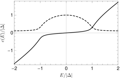
Figure 1: The function $c(E)$ as defined in Eq. (25g) frequently appears in expressions associated with stationary solutions. The solid line represents the real part and the dashed line the imaginary part. The Thouless energy was taken as $E_{\rm Th}=0.1\,|\Delta|$.

With the aide of the prescription below Eq. (11) for choosing the eigenvalues of $G$, one then readily finds for the retarded and advanced Green functions

$$R(E) = \frac{1}{c(E)}\left(\begin{array}[]{cc}E+iE_{\rm Th}&-\Delta\\ \Delta^{*}&-E-iE_{\rm Th}\end{array}\right),$$ (25c)

$$A(E) = \frac{1}{c(-E)}\left(\begin{array}[]{cc}E-iE_{\rm Th}&-\Delta\\ \Delta^{*}&-E+iE_{\rm Th}\end{array}\right),$$ (25f)

$$c(E) = \sqrt{(E+iE_{\rm Th})^{2}-|\Delta|^{2}}.$$ (25g)

The function $c(E)$, which we will frequently encounter, is defined with branch cuts along the lines $E_{\pm}=\pm|\Delta|\pm x-iE_{\rm Th}$ with $x$ real and positive. The branch with $\lim_{E\in R\to\pm\infty}c(E)/E=1$ is taken. Considered as a function of real $E$, the real part of $c(E)$ is odd, and the imaginary part is even and positive so that

$$c(E)^{*}=-c(-E).$$ (26)

The real and imaginary parts of $c(E)$ is plotted for real $E$ in Fig. 1.

Figure 2: The density of states of the superconducting island (Eq. 27) for finite Thouless energy (solid line). The dashed line shows the density of states of the isolated superconducting island with the same $|\Delta|$, while the horizontal dot-dashed line shows the density of states of the normal island. A value of $E_{\rm Th}=0.1\,|\Delta|$ was used.

Note that $R(E)^{2}=A(E)^{2}=\eta_{0}$ as required by Eq. 12. In general the superconducting density of states is $\varrho(E)={\rm Tr}\,\eta_{3}\left[R(E)-A(E)\right]/2\delta_{s}$ so that we find from the solutions for $R$ and $A$ (Eq. 25)

$$\varrho(E)=\frac{2}{\delta_{s}}{\rm Re}\left[\frac{E+iE_{\rm Th}}{c(E)}\right].$$ (27)

The density of states for an isolated superconductor has singularities at energies $E=\pm|\Delta|$ of the form $1/\sqrt{E^{2}-|\Delta|^{2}}$. The coupling to the leads regularizes the singularities at an energy scale of $E_{\rm Th}$. Furthermore, whereas the density of states of the isolated superconductor vanishes for energies $|E|<|\Delta|$, the coupling to the leads softens the gap so that there are some states for energies $|E|<|\Delta|$ as shown in Fig. 2.

The next step is to solve Eq. (24b) for $K(E)$. Here we use the fact that $R(E)K(E)A(E)=-K(E)$, which follows from the requirement that $G^{2}=I$ (Eq. 12). Note also that $R(E)=M_{R}(E)/c(E)$ and $A(E)=M_{A}(E)/c(-E)$. Using these identities and multiplying Eq. (24b) from the left by $R(E)$, we find

$$K(E)=\frac{1}{c(E)+c(-E)}\left[M_{K}(E)-R(E)M_{K}(E)A(E)\right].$$ (28)

After some algebra we obtain

$$K(E)=\left(\begin{array}[]{cc}K^{(1)}(E)&K^{(2)}(E)\\ -K^{(2)}(E)^{*}&K^{(1)}(-E)\end{array}\right),$$ (29)

where

$$K^{(1)}(E) = \delta_{s}\varrho(E)\sigma(E)-\frac{|\Delta|^{2}}{E}{\rm Re}\left[\frac{1}{c(E)}\right]\left[\sigma(E)+\sigma(-E)\right],$$ (30a)

$$K^{(2)}(E) = -\Delta{\rm Re}\left[\frac{1}{c(E)}\right]\left\{\left[\sigma(E)-\sigma(-E)\right]-\frac{iE_{\rm Th}}{E}\left[\sigma(E)+\sigma(-E)\right]\right\}.$$ (30b)

Having obtained $K(E)$ we can find $|\Delta|$ and $\mu$ from the self-consistency condition Eq. (15). Below we write the real and imaginary parts of the self-consistency equation separately. The real part reads

$$0=\int dE\left\{{\rm Re}\left[\frac{1}{c(E)}\right]\frac{\sigma(E)-\sigma(-E)}{2}-\frac{1}{\sqrt{E^{2}+\Delta_{0}^{2}}}\right\},$$ (31)

while the imaginary part reads

$$0=\int dE\,\frac{1}{E}{\rm Re}\left[\frac{1}{c(E)}\right]\left[\sigma(E)+\sigma(-E)\right].$$ (32)

These integrals can be done explicitly. We use the identities

$$\int_{0}^{E}dE^{\prime}\,{\rm Re}\frac{1}{c(E^{\prime})}=F_{R}(E)-F_{R}(0),$$ (33a)

$$\int_{0}^{E}dE^{\prime}\,\frac{1}{E^{\prime}}{\rm Re}\frac{1}{c(E^{\prime})}=\frac{1}{\sqrt{E_{\rm Th}^{2}+|\Delta|^{2}}}F_{I}(E),$$ (33b)

where

$$F_{R}(E) = \ln\left|\frac{E+iE_{\rm Th}+c(E)}{\Delta_{0}}\right|,$$ (34a)

$$F_{I}(E) = \arctan\left[\frac{{\rm Re}[c(E)]}{\sqrt{E_{\rm Th}^{2}+|\Delta|^{2}}}\right].$$ (34b)

Here the branch for which $-\pi/2<\arctan(x)<\pi/2$ is implied. Thus we obtain the transcendental equations

$$0=(1-\gamma)F_{R}(\tfrac{eV}{2}+\mu)+(1+\gamma)F_{R}(\mu-\tfrac{eV}{2}),$$ (35a)

$$0=(1-\gamma)F_{I}(\tfrac{eV}{2}+\mu)+(1+\gamma)F_{I}(\mu-\tfrac{eV}{2}),$$ (35b)

that determine $|\Delta|$ and $\mu$ for given $V$, $E_{\rm Th}$ and $\gamma$. Below we solve these equations analytically in certain limiting cases and numerically for more general cases. Only the amplitude of $\Delta$ is fixed by these equations. By choosing the appropriate gauge [cf. Eq. (14b)], we can set the phase of $\Delta$ to any value. In the rest of this section we therefore drop the absolute value notation, and take $\Delta$ real and positive.

Before explicitly finding $\Delta$ and $\mu$, we calculate the current from Eq. (17) and the solution for $K(E)$. Assuming that the self-consistency equation (Eq. 32) is fulfilled, we find that the current $I_{r}$ from the superconductor to the right lead equals minus the current $I_{l}$ from the superconductor to the left lead, as it should. For the current $I=I_{r}=-I_{l}$ from the left lead to the right lead we find

$$I = \frac{(1-\gamma^{2})eE_{\rm Th}}{2}\int_{\mu-\tfrac{eV}{2}}^{\mu+\tfrac{eV}{2}}dE\,\varrho(E)$$ (36)

$$= \frac{G_{N}}{e}{\rm Re}\left[c(\mu+\tfrac{eV}{2})-c(\mu-\tfrac{eV}{2})\right].$$

Here $G_{N}$ is the series conductance of the tunneling barriers to the leads

$$G_{N}=\left[G_{l}^{-1}+G_{r}^{-1}\right]^{-1},$$ (37)

and $G_{l}$ and $G_{r}$ are the junction conductances given in Eq. (17).

Now we investigate the transcendental equations (Eqs. 35) for $\mu$ and $\Delta$. There are three parameters, namely $E_{\rm Th}$, $\gamma$ and $V$ that determine the solution. Two of these, $E_{\rm Th}$ and $\gamma$, are fixed for a given device, while the voltage $V$ can be varied for a given device. (Recall that $E_{\rm Th}$ measures the overall coupling to the leads, while $\gamma$ measures the degree of asymmetry between the two lead couplings.) Hence it is natural to specify values for $E_{\rm Th}$ and $\gamma$ and then consider $\Delta$, $\mu$ and $I$ as functions of $V$. In Fig. 3 we show four curves of $\Delta$ versus $V$, each corresponding to a different choice of the parameters $E_{\rm Th}$ and $\gamma$. In Fig. 4 we show the corresponding curves of $\mu$ versus $V$.

Figure 3: The order parameter $\Delta$ versus voltage $V$, for given $E_{\rm Th}$ and $\gamma$. Curves $A$, $B$, $C$ and $D$ respectively correspond to $E_{\rm Th}=0.35\Delta_{0}$ and $\gamma=0.2$; $E_{\rm Th}=0.2\Delta_{0}$ and $\gamma=0.075$; $E_{\rm Th}=0.1\Delta_{0}$ and $\gamma=0.1$; and $E_{\rm Th}=0.01\Delta_{0}$ and $\gamma=0.3$.

Figure 4: The chemical potential $\mu$ versus voltage $V$, for given $E_{\rm Th}$ and $\gamma$. Curves $A$, $B$, $C$ and $D$ correspond to the same parameter values as in Fig. 3.

Let us firstly note the general trend that increasing $E_{\rm Th}$ leads to a smaller order parameter. The reason for this is that $E_{\rm Th}^{-1}$ is the typical time an electron remains in the superconductor. The shorter this time (the larger $E_{\rm Th}$) the harder it is for electrons to form Cooper pairs, and superconductivity is inhibited. Secondly, note that at large enough $E_{\rm Th}$ the order parameter is a decreasing function of $V$. We can therefore obtain the critical Thouless energy $E_{\rm Th}^{(c)}$ beyond which superconductivity vanishes by setting $V$ to zero and asking how large can we make $E_{\rm Th}$ before $\Delta$ becomes zero.

In the case of $V=0$, the self-consistency equations are solved by $\mu=0$ and

$$\Delta=\left\{\begin{array}[]{lr}\Delta_{0}\sqrt{1-\frac{2E_{\rm Th}}{\Delta_{0}}}&E_{\rm Th}<\Delta_{0}/2\\ 0&E_{\rm Th}>\Delta_{0}/2\end{array}\right..$$ (38)

From this we conclude that the critical Thouless energy is $E_{\rm Th}^{(c)}=\Delta_{0}/2$.

Having established the range of $E_{\rm Th}$ in which superconductivity persists, we now take a closer look at $\Delta$ as a function of $V$. We have chosen the parameters of the four solutions in Fig. 3 to show all the different possible shapes that curve of $\Delta$ versus $V$ can take. We see that at a given voltage $V$ there can be either zero, one, two or three non-zero solutions $\Delta$.

To characterize the different types of curve, we consider $V$ as a function of $\Delta$ on the interval $\Delta\in[0,\Delta_{0}\sqrt{1-2E_{\rm Th}/\Delta_{0}}]$. In curves of the type $A$ in Fig. 3, $V$ is a monotonically decreasing function of $\Delta$. In contrast, curves of type $B$, $C$ and $D$ have local extrema. A curve of type $B$ has a local minimum at the left boundary $\Delta=0$ of the $\Delta$ interval on which the function $V(\Delta)$ is defined. Then the curve reaches a maximum at some intermediate value $\Delta_{1}$, before dropping to zero at the right boundary $\Delta=\Delta_{0}\sqrt{1-2E_{\rm Th}/\Delta_{0}}$. Curves $C$ and $D$ are distinguished from curve $B$ by the fact that $V$ reaches a local maximum instead of a minimum at the left boundary $\Delta=0$ of the $\Delta$ interval. There is another local maximum at intermediate $\Delta_{1}$ before $V$ drops to zero at $\Delta=\Delta_{0}\sqrt{1-2E_{\rm Th}/\Delta_{0}}$. In curves of type $C$, the absolute maximum of $V$ as a function of $\Delta$ is at the intermediate value $\Delta_{1}$ while for curves of type $D$ the absolute maximum of $V$ is at $\Delta=0$.

Next we ask how the $E_{\rm Th}$—$\gamma$ parameter space is divided into regions $A$, $B$, $C$ and $D$ corresponding to the respective types of solution of the self-consistency equations. Specifically, which regions share a mutual border? Assuming that the function $V(\Delta)$ changes smoothly as $E_{\rm Th}$ and $\gamma$ are varied, the transitions $A\leftrightarrow B$, $B\leftrightarrow C$, $C\leftrightarrow D$ and $D\leftrightarrow A$ are possible. The transition $A\leftrightarrow C$ is not possible. Whenever one tries to smoothly deform a curve of type $A$ in Fig. 3 to a curve of type $C$, one invariably reaches a curve of type $B$ or $D$ during an intermediate stage of the deformation. Similarly the transition $B\leftrightarrow D$ is impossible. A smooth deformation of a curve of type $B$ into one of type $D$ passes through an intermediate stage where the curve is of types $A$ or $C$. To illustrate these ideas we consider a polynomial equation of the form

$$\frac{\tilde{V}}{\Delta_{0}}=\frac{V_{0}}{\Delta_{0}}-\frac{1}{6}\left(\frac{\Delta}{\Delta_{0}}\right)^{6}-\frac{a}{4}\left(\frac{\Delta}{\Delta_{0}}\right)^{4}-\frac{b}{2}\left(\frac{\Delta}{\Delta_{0}}\right)^{2}.$$ (39)

We ask what are the respective regions of the $a$—$b$ plane in which $\tilde{V}(\Delta)$ is a curve of type $A$, $B$, $C$ and $D$. Region $A$, where $\tilde{V}(\Delta)$ is of type $A$, is given by $a>0,\,b>0$ or $a<0,\,b>a^{2}/4$. Region $B$ where $\tilde{V}(\Delta)$ is of type $B$ consists of all points $(a,b)$ such that $b<0$. Region $C$ consists of all points $(a,b)$ such that $a<0$ and $0<b<3a^{2}/16$. Region $D$ consists of all points $(a,b)$ such that $a<0$ and $3a^{2}/16<b<a^{2}/4$. The regions and their borders are shown in the inset in Fig. 5. The most pertinent feature of the figure is that the four distinct regions meet in the single point $a=b=0$.

Based on a combination of numerical and analytical results we have concluded that the $E_{\rm Th}$—$\gamma$ parameter space has a very similar topology to this polynomial example. (In principle it could have differed from the polynomial example by having disconnected regions of the same type, for instance two islands of region $D$, one embedded in a sea of region $A$, the other in a sea of region $C$.) Fig. 5 is a schematic diagram of how the $E_{\rm Th}$—$\gamma$ parameter space is partitioned into regions $A$, $B$, $C$ and $D$. The following features of the diagram are conjectures based on numerical evidence: (1) The regions of types $A$, $B$, $C$ and $D$ are simply connected. (2) The border between regions $A$ and $D$ starts at the corner $\gamma=1$, $E_{\rm Th}=0$. Other features are deduced from analytical results: (1) The line $\gamma=0$, $E_{\rm Th}<\Delta_{0}/2\sqrt{2}$ belongs to region $B$. (2) The line $\gamma=0$, $\Delta_{0}/2\sqrt{2}<E_{\rm Th}<\Delta_{0}/2$ belongs to region $A$. (3) For $E_{\rm Th}>\Delta_{0}/2$ the system is in the normal state while it is superconducting for $E_{\rm Th}<\Delta_{0}/2$. 4) The border of regions $D$ and $C$ meets the border of region $B$ and $C$ at $E_{\rm Th}=0$, $\gamma=0$.

Figure 5: Schematic diagram of the partitioning of the $E_{\rm Th}$—$\gamma$ parameter space into regions where the curve of $\Delta$ versus $V$ is of the types $A$, $B$, $C$ and $D$ (Fig. 3). The regions $A$, $B$, $C$, and $D$ meet at point $Q$. The line $E_{\rm Th}=\Delta_{0}/2$ separates the normal and superconducting regions of parameter space. The dots in the figure indicate the parameter values that correspond to the curves in Fig. 3. The inset shows the regions $A$, $B$, $C$, and $D$ in the parameter space $a$—$b$ of the polynomial $\tilde{V}(\Delta)$ of Eq. (39). The topology of the $E_{\rm Th}$—$\gamma$ parameter space of the superconductor in the region of the point $Q$ can be understood by considering the topology of the parameter space of the polynomial.

In region $D$, superconductivity can persist up to voltages that are large compared to $\Delta_{0}$. For given $E_{\rm Th}$ and $\gamma$ there is however always a critical voltage $V_{c}$ beyond which superconductivity ceases. (This is a second order phase-transition.) For the voltage $V_{c}$ we have obtained the following analytical result from Eq. (35). At finite $\gamma$ and for $E_{\rm Th}$ sufficiently small, $V_{c}$ obeys the power law

$$V^{(c)}=\frac{\Delta_{0}}{2e}\left[\frac{2E_{\rm Th}}{\Delta_{0}}\sec\frac{\pi\lambda}{2}\right]^{-\frac{1}{\lambda}},\hskip 5.69054pt\lambda=\frac{1-|\gamma|}{1+|\gamma|}.$$ (40)

This power law is valid as long as $V^{(c)}\gg\Delta_{0}/e$. It is from this result that we are able to conclude that the region of finite $\gamma$ and infinitesimal $E_{\rm Th}$ belongs to region $D$.

Another analytical result can be obtained for the case of perfectly symmetric coupling to the leads, i.e. $\gamma=0$. In this case, Eq. (35b) is solved by $\mu=0$ and the relation between $\Delta$ and $V$ can be stated as

$$eV=\Delta_{0}\left(1+\frac{\Delta^{2}}{\Delta_{0}^{2}}\right)\sqrt{1-\frac{4E_{\rm Th}^{2}/\Delta_{0}^{2}}{\left(1-\frac{\Delta^{2}}{\Delta_{0}^{2}}\right)^{2}}}.$$ (41)

This result is plotted for several values of $E_{\rm Th}$ in Fig. 6. It is from this result that we are able to conclude that the line segment $\gamma=0$, $0<E_{\rm Th}<\Delta_{0}/2\sqrt{2}$ belongs to region $B$ while the line segment $\gamma=0$, $\Delta_{0}/2\sqrt{2}<E_{\rm Th}<\Delta_{0}/2$ belongs to region $A$. The $E_{\rm Th}\to 0$ limit of Eq. (41) can be obtained by considering a bulk superconductor and assuming a quasi-particle distribution function $n(E)=(\theta(-eV/2-E)+\theta(eV/2-E))/2$. It is also worth noting that the same result is obtained for a T-junction where the stem of the T is a superconductor and the bar a voltage-biased dirty normal metal wire.Kei06

Figure 6: The order parameter $\Delta$ versus voltage $V$ for symmetric coupling to the leads, i.e. $\gamma=0$, according to Eq. (41). Different curves correspond to different $E_{\rm Th}$. From the top curve to bottom curve we took $E_{\rm Th}/\Delta_{0}=.01$, $0.14$, $0.26$, $1/2\sqrt{2}(\simeq 0.35)$, $0.42$ and $0.47$. The curve corresponding to $E_{\rm Th}=1/2\sqrt{2}\Delta_{0}$ is plotted thicker than the others. For smaller $E_{\rm Th}$ are of type $B$ with two non-zero values for $\Delta$ at some voltages. For larger $E_{\rm Th}$, curves are of type $A$, with at most one non-zero $\Delta$ at every voltage.

Finally, we consider the $I-V$ curves associated with the solutions $\Delta$ and $\mu$ of Figs. 3 and 4. The results are shown in Fig. 7. From these curves we can infer the results that will be obtained in an experiment in which the voltage $V$ is swept adiabatically from zero to several $\Delta_{0}/e$ and back to zero. In region $A$ of parameter space there is a single current associated with each voltage. At some voltage $V_{+}$ of order $\Delta_{0}/e$ the system makes a phase transition to the normal state, but this does not lead to a discontinuity in the current versus voltage curve. In contrast, in regions $B$, $C$ and $D$, the current will make discontinuous jumps as the voltage is swept. Hysteresis will also be observed. Suppose the device is in region $B$ of parameter space. As $V$ is swept from $0$ upwards, a voltage $V_{+}$ is crossed where the current makes a finite jump. After the jump, the system is in the normal state and the current is $G_{N}V$. ($G_{N}$ is the normal state conductance of the setup, cf. Eq. 37.) On the backward sweep from $V>V_{+}$ to zero, the system remains normal when $V_{+}$ is reached. At some voltage $V_{-}<V_{+}$ the current jumps from its value $G_{N}V_{-}$ in the normal state to a smaller value, signaling the onset of superconductivity. The behavior of the system in region $C$ of parameter space is similar. The upward sweep of the voltage produces a jump in the current at a voltage $V_{+}$. After the jump the system is normal and the current is given by $I=G_{N}V$. The difference from region $B$ appears when the voltage is swept back from $V_{+}$ to zero. At some voltage smaller than $V_{+}$ the current starts deviating from its value in the normal state, but there is no discontinuous jump yet. Even so, the system has turned superconducting. When the jump in current now occurs at $V_{-}<V_{+}$, the system switches between two different superconducting states. Finally, for parameters in region $D$, the voltage sweep produces results similar to that in region $C$. The difference between regions $C$ and $D$ is that in $D$ the system also jumps between two superconducting states at $V_{+}$ during the forward sweep.

Figure 7: The current $I$ through the superconductor versus the voltage $V$ across it. Curves $A$, $B$, $C$ and $D$ correspond to the respective parameter values quoted in Figs. 3 and 4. The dashed line shows the current through the system in the absence of superconductivity.

IV Dynamics

We concluded the previous section with a discussion of hysteresis in the current–voltage characteristic of the superconducting island. The conclusions we drew rely on the assumption that after the system is perturbed by a change in the bias voltage, it relaxes into a stationary state. The validity of this assumption is by no means obvious, since the system is driven (by the bias voltage) and the stationary state is not an equilibrium state. Frankly, our own initial expectation was that the presence of a bias voltage would cause the dynamics of $|\Delta(t)|$ to be quasi-periodic or chaotic. We therefore did numerical simulations in order to investigate the dynamics of $|\Delta(t)|$ in the presence of a bias voltage. Our main result is this: Suppose the bias voltage assumes the constant value $V_{f}$ for times $t>t_{f}$. Then (contrary to our original expectations) at $t\gg t_{f}$ the superconductor will always be found in one of the stationary states associated with $V_{f}$. This is true regardless of the history of the system prior to $t<t_{f}$. In particular, the time dependence of the bias voltage prior to $t_{f}$ does not matter. Nor does the state of the superconductor prior to $t_{f}$ matter. Only when there is more than one non-zero stationary solution associated with $V_{f}$ does the history of the system have any baring on its final state. In this case, the history of the system determines which of the possible stationary states eventually becomes the final state of the superconductor. For slowly varying voltages, the predictions of the previous section regarding hysteresis are confirmed. In this section we discuss the numerics that yielded the above results.

For the purpose of numerics we find it advantageous not to take the sum over levels of the Green function as we did in the previous sections. Instead we work with the Green functions of each individual level. The advantage of this scheme is that it allows us to work with ordinary differential equations. From these differential equations it is straight-forward to construct a time-series in which the next element can be calculated if the present elements are known. As far as we can see, no such ‘local in time’ update equations exist for the Green functions summed over levels. Naturally there are disadvantages to working with the individual level Green functions as well; the number of equations to be solved numerically is increased significantly. As a result the calculation is computationally expensive and therefore time-consuming.

The Green functions of the individual levels obey the equations

$$(H_{m}-\Sigma)G_{m}=G_{m}(H_{m}-\Sigma)=I.$$ (42)

Here $H_{m}$ differs from the operator $H$ that appeared in Eq. (5) in that it contains the energy $\varepsilon_{m}$ of level $m$. It is explicitly given by

$$H_{m}(t,t^{\prime}) = \tau_{0}\otimes\eta_{3}\,\delta(t-t^{\prime})\left[i\partial_{t}-h_{m}(t)\right],$$ (43a)

$$h_{m}(t) = \left(\begin{array}[]{cc}\varepsilon_{m}-\mu_{s}(t)&\Delta(t)\\ \Delta(t)^{*}&\mu_{s}(t)-\varepsilon_{m}\end{array}\right).$$ (43d)

The operator $h_{m}(t)$ is the time-dependent Bogoliubov-de Gennes Hamiltonian.deG66 The self-energy $\Sigma$ is the same as in Sect. II.2.

We measure energies from a point halfway between the chemical potentials of the leads. As a result the phases $\phi_{j}(t)$ that appear in the reservoir self-energies are $\phi_{r(l)}(t)=+(-)\phi(t)/2$ where $\phi$ is related to the voltage $V$ by $V(t)=\partial_{t}\phi(t)/e$.

We parameterize the Green functions in terms of a set of auxiliary functions. This eliminates some redundancies that are present due to symmetries of the equations of motion. We start by noting that since the retarded and advanced Green functions are related by Eq. (1g), we do not need to consider both. We work with the retarded Green function. We define a matrix $r_{m}(t,\tau)$ that is related to $R_{m}(t,t-\tau)$ by the equation

$$R_{m}(t,t-\tau) = i\,\eta_{3}~{}r_{m}(t,\tau),$$ (44a)

$$r_{m}(t,\tau) = r_{m}^{(0)}(t,\tau)\,\eta_{0}+i\,\bm{r}_{m}(t,\tau)\cdot\bm{\eta}.$$ (44b)

Here the component $r_{m}^{(0)}(t,\tau)$ of $r_{m}(t,\tau)$ is a scalar function whereas the other three components are grouped into a vector $\bm{r}_{m}(t,\tau)$ such that

$$\bm{r}_{m}(t,\tau)=\left(r^{(1)}_{m}(t,\tau),r^{(2)}_{m}(t,\tau),r^{(3)}_{m}(t,\tau)\right).$$ (45)

The vector $\bm{\eta}=(\eta_{1},\eta_{2},\eta_{3})$ contains the Pauli matrices in Nambu space. Before the voltage bias between the leads is established, (i.e. for $t\leq 0$ and all $\tau$), the functions $r_{m}^{(0)}(t,\tau)$ and $\bm{r}_{m}(t,\tau)$ are real. When the equations of motion (42) for the retarded Green function are rewritten in terms $r^{(0)}$ and $\bm{r}$, we find that their reality is preserved at all times.

Next we consider the Keldysh Green function. In order to calculate the time-evolution of the order parameter we only need to know the Keldysh Green function at coinciding times. Here the parameterization

$$K_{m}(t,t)=i\,\eta_{3}~{}\bm{k}_{m}(t)\cdot\bm{\eta},$$ (46)

in terms of a real vector

$$\bm{k}_{m}(t)=\left(k^{(1)}_{m}(t),k^{(2)}_{m}(t),k^{(3)}_{m}(t)\right),$$ (47)

is respected by the initial condition and preserved by the equations of motion.

From the equations of motion (Eq. 42) we derive differential equations

$$\frac{d}{dt}r_{m}(t,\tau)=b_{m}(t)r_{m}(t,\tau)-r_{m}(t,\tau)b_{m}(t-\tau),$$ (48)

$$\frac{d}{dt}\bm{k}_{m}(t)+2\bm{b}_{m}(t)\times\bm{k}_{m}(t)+2E_{\rm Th}\bm{k}_{m}(t)=4E_{\rm Th}\bm{f}_{m}(t),$$ (49)

for the matrix $r_{m}(t,\tau)$ and the vector $\bm{k}_{m}(t)$. The equation (49) with $E_{\rm Th}=0$ was studied in Refs. Bar06, ; Yuz05, . In these references the dynamics of the order parameter of an isolated superconductor was calculated. We see that coupling the system to leads introduces two terms proportional to $E_{\rm Th}$. One (on the left-hand side of Eq. (49)) can be considered a damping term and is proportional to ${\bm{k}}_{m}(t)$. The other (on the right-hand side of Eq. (49)) can be considered a driving or source term.

In Eq. (49), $b_{m}(t)$ is a matrix and $\bm{b}_{m}(t)$ a vector such that

$$b_{m}(t) = i\,\bm{b}_{m}(t)\cdot\bm{\eta},$$ (50a)

$$\bm{b}_{m}(t) = \left({\rm Re}\,\Delta(t),-{\rm Im}\,\Delta(t),\mu_{s}(t)-\varepsilon_{m}\right).$$ (50b)

The equation for $\bm{k}_{m}(t)$ contains a source term $4E_{\rm Th}\bm{f}_{m}(t)$. The vector $\bm{f}_{m}(t)$ is given by

$$\bm{f}_{m}(t)=\int_{0}^{\infty}d\tau\,\left[r_{m}^{(0)}(t,\tau)\bm{s}(t,\tau)-\bm{r}_{m}(t,\tau)s^{(0)}(t,\tau)-\bm{r}_{m}(t,\tau)\times\bm{s}(t,\tau)\right].$$ (51)

In this equation the scalar function $s^{(0)}(t,\tau)$ and the vector $\bm{s}(t,\tau)$ parameterize the Keldysh component of the self-energy as follows

$$\Sigma_{K}(t,t^{\prime}) = 2E_{\rm Th}\,\eta_{3}~{}s(t,\tau),$$ (52a)

$$s(t,\tau) = s^{(0)}(t,\tau)\,\eta_{0}+i\bm{s}(t,\tau)\cdot\bm{\eta}.$$ (52b)

Referring back to Sec. II, where $\Sigma_{K}$ is expressed in terms of the Fourier transform of the reservoir filling factors, we find explicitly

$$s^{(0)}(t,\tau) = \frac{1}{\pi}\mathcal{P}\left(\frac{1}{\tau}\right)\cos\frac{\phi(t)-\phi(t-\tau)}{2},$$ (53a)

$$\bm{s}(t,\tau) = -\frac{\gamma}{\pi\tau}\left(0,0,\sin\frac{\phi(t)-\phi(t-\tau)}{2}\right).$$

By imposing self-consistency, the order parameter $\Delta(t)$ is expressed in terms of the components of $\bm{k}_{m}(t)$ as

$$\Delta(t)=\frac{g\delta_{s}}{2}\sum_{m=-\Omega}^{\Omega}k_{m}^{(1)}(t)-ik_{m}^{(2)}(t),$$ (54)

where the number of levels on the island is $2\Omega+1$. This makes the differential equations non-linear, since they contain terms in which $\Delta(t)$ multiplies ${\bm{k}}_{m}$ and $r$. We eliminate the dimensionless pairing strength $g$ and the mean level spacing $\delta_{s}$ in favor of $\Delta_{\rm eq}$, the order parameter of the island in equilibrium, by means of the equilibrium self-consistency relation

$$\frac{2}{g\delta_{s}}=\sum_{m=-\Omega}^{\Omega}\frac{1}{\xi_{m}}\frac{2}{\pi}\arctan\frac{\xi_{m}}{E_{\rm Th}},$$ (55)

where

$$\xi_{m}=\sqrt{\varepsilon_{m}^{2}+\Delta_{\rm eq}^{2}}.$$ (56)

As with $\Delta(t)$, the chemical potential $\mu_{s}(t)$ is determined by a self-consistency equation. The chemical potential takes into account the work that must be performed against the electric field of the excess charge on the superconductor in order to add more charge. Thus $\mu_{s}(t)$ is related to the charge of the island by $\mu_{s}(t)=e[Q(t)-Q_{0}]/C$ where $C$ is the capacitance of the island. In this equation $Q_{0}$ represents the fixed positive background charge and $Q(t)$ is the combined charge of all the electrons on the island. Since the differential equations (48) and (49) only depend on the difference $\mu_{s}(t)-\mu_{s}(t-\tau)$, the positive background charge need not be specified. The charge $Q(t)$ is related to the Keldysh Green function. Indeed, the average number $n_{m}(t)$ of electrons (with spin-degeneracy included) in level $m$ at time $t$ is given by $n_{m}(t)=(1-i{\rm Tr}[K_{m}(t,t)])/2$. Hence $\mu_{s}(t)$ is related to $\bm{k}_{m}$ by the equation

$$\mu_{s}(t)-\mu_{s}(t-\tau)=\frac{e^{2}}{2C}\sum_{m=-\Omega}^{\Omega}k_{m}^{(3)}(t)-k_{m}^{(3)}(t-\tau).$$ (57)

Finally, we have to specify the initial conditions for $r_{m}(t,\tau)$ and $\bm{k}_{m}(t)$. We will assume for our simulations that the voltage between the reservoirs is zero and the system is in zero-temperature equilibrium for times $t<0$. The corresponding initial condition at $t=0$ is

$$r^{(0)}_{m}(0,\tau) = -\theta(\tau)e^{-E_{\rm Th}\tau}\cos(\xi_{m}\tau),$$ (58a)

$$\bm{r}_{m}(0,\tau) = \theta(\tau)e^{-E_{\rm Th}\tau}\frac{\sin(\xi_{m}\tau)}{\xi_{m}}\left(-\Delta_{\rm eq},0,\varepsilon_{m}\right),$$

$$\bm{k}_{m}(0) = \frac{1}{\xi_{m}}\frac{2}{\pi}\arctan\frac{\xi_{m}}{E_{\rm Th}}\left(\Delta_{\rm eq},0,-\varepsilon_{m}\right).$$ (58c)

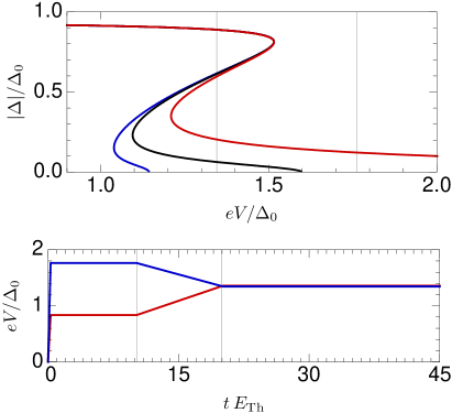
Figure 8: Top panel: The stationary solutions for $\Delta$ vs. the bias voltage $V$, corresponding to the parameters used in generating Fig. 9. The outer curve (red) corresponds to $E_{\rm Th}=0.069\Delta_{0}$ and $\gamma=0.2$. The middle curve (black) corresponds to $E_{\rm Th}=0.069\Delta_{0}$ and $\gamma=0.1$. The inner curve (blue) corresponds to $E_{\rm Th}=0.069\Delta_{0}$ and $\gamma=0.05$. The vertical lines indicate $V_{f}$ and $V_{2}$. ($V_{1}$ is beyond the left edge of the figure.) Bottom panel: The time-dependence of the voltage. The upper (blue) curve corresponds to the blue curves of $\Delta$ vs. $t$ in Fig. 9. The lower (red) curve corresponds to the red curves of $\Delta$ vs. $t$ in Fig. 9.

We are now ready to study the time-evolution of $\Delta(t)$ when a non-zero bias voltage $V(t)$ between the leads is present for times $t>0$. In the calculations we report on here, we worked with $E_{\rm Th}=0.069\,\Delta_{0}$ and three different $\gamma$, namely $\gamma=0.05$, $\gamma=0.1$ and $\gamma=0.2$. These all correspond to points from regions $C$ and $D$ in the $E_{\rm Th}$–$\gamma$ parameter space of Fig. 5. Hence, for each of the parameter choices, there is a bias voltage interval $[V_{-},V_{+}]$ where there are more than one non-zero stationary solutions for $|\Delta|$. The three curves of stationary $|\Delta|$ versus $V$, corresponding to the different parameter choices, are plotted in the top panel of Fig. 8.

For given $E_{\rm Th}$ and $\gamma$ we did two numerical runs with different time-dependent voltages $V(t)$. The two voltages are plotted as functions of time in the bottom panel of Fig. 8. In the first run we start by rapidly establishing a bias voltage $V_{1}<V_{-}$. Rapid here means $dV/dt\gg\Delta_{0}E_{\rm Th}/e$. In this case $V$ changes by an amount of order $\Delta_{0}/e$ — the scale at which the stationary solution for $|\Delta|$ depends on $V$ — in a time that is short compared to the relaxation time $E_{\rm Th}^{-1}$. (Slow refers to the opposite limit.) We then keep the voltage constant at $V_{1}$ for a length of time of several $E_{\rm Th}$. This time-interval is long enough for any transient behavior induced by the rapid change of $V(t)$ to disappear. We then slowly increase the bias voltage until we reach a bias voltage $V_{f}\in[V_{-},V_{+}]$ for which more than one non-zero stationary solutions exist. In the second run we start by rapidly establishing a bias voltage $V_{2}>V_{+}$. We keep the voltage fixed at $V_{2}$ for a time of several $E_{\rm Th}^{-1}$. We then slowly decrease the voltage to $V_{f}$. The values of $V_{1}$, $V_{2}$ and $V_{f}$ were chosen $V_{1}=0.83\Delta_{0}$, $V_{2}=1.76\Delta_{0}$ and $V_{f}=1.34\Delta_{0}$. The calculations were performed with $501$ equally spaced levels with level spacing $\delta_{s}=0.018\Delta_{0}$ and the capacitance was chosen $C=0.1\,e^{2}/\Delta_{0}$.

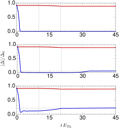
Figure 9: The amplitude of the order parameter as a function of time. All curves are for $E_{\rm Th}=0.069\Delta_{0}$. The top, middle and bottom panels correspond to $\gamma=0.05$, $\gamma=0.1$ and $\gamma=0.2$ respectively. The red curves correspond to a voltage that is increased from $V_{1}=0.83\Delta_{0}$ to $V_{f}=1.34\Delta_{0}$. The blue curves correspond to the voltage being decreased from $V_{2}=1.76\Delta_{0}$ to $V_{f}=1.34\Delta_{0}$. The vertical lines indicate the time-interval in which the voltage changes from either $V_{1}$ or $V_{2}$ to $V_{f}$. The thin horizontal lines correspond to the stationary values of $|\Delta|$ for a bias voltage $V=V_{f}$ as calculated from Eq. (35).

The resulting $|\Delta|$ are plotted as functions of time in Fig. 9. They firstly show that after the initial rapid change in the bias voltage the system always relaxes into a stationary state consistent with the new voltage. The relaxation takes a time of the order $E_{\rm Th}^{-1}$. Secondly, if the system is in a stationary state, and the bias voltage is changed slowly then $|\Delta(t)|$ adiabatically tracks the stationary solution corresponding to the instantaneous value of the voltage. This is seen most clearly in Fig. 10 where we plot $|\Delta(t)|$ as a function of $V(t)$ and compare this to the stationary $|\Delta|$ vs. constant $V$ curves. Our prediction about hysteresis is confirmed. Systems with different histories end up in different stationary states at the same voltage bias. If the voltage is slowly swept from a small initial voltage to $V_{f}\in[V_{-},V_{+}]$ a stationary state with a large value for $|\Delta|$ is reached. If the voltage is swept from a large initial voltage to $V_{f}\in[V_{-},V_{+}]$, a stationary state is reached that corresponds to a small value of $|\Delta|$. We must mention here that we observe some slow drift (too slow to be visible in Fig. 9) in $|\Delta|$ after the voltage has reached $V_{f}$. The value of $|\Delta|$ seems to increase linearly at a rate $d|\Delta|/dt\sim 10^{-4}\Delta_{0}^{2}$. Within the numerical accuracy of the calculation, this is negligible and we believe the drift is simply an artifact of the numerics.

In our data there is one exception to the rule of adiabatic evolution. In the middle panel of Fig. 9, $|\Delta(t)|$ takes much longer that $E_{\rm Th}^{-1}$ to respond when the voltage is changed from $V_{2}$ to $V_{f}$. Hence, $|\Delta(t)|$ as a function of $V(t)$ does not track the stationary solution in this instance. The reason is the following: For a voltage $V=V_{2}$, the only stationary solution has $\Delta=0$. When the voltage is decreased to $V_{f}$, a non-zero stationary solution for $\Delta$ exists. However $\Delta=0$ is still a valid state, albeit unstable. The time it takes the system to diverges from the unstable state is not determined by $E_{\rm Th}$ but rather by small numerical errors that perturb the unstable state.

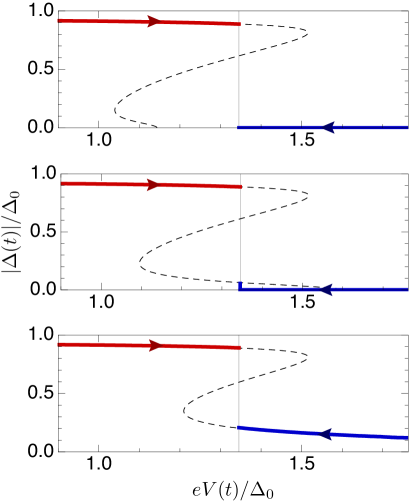
Figure 10: The amplitude of the order parameter $|\Delta(t)|$ as a function of voltage $V(t)$. The parameter values of the three panels are the same as those in Fig. 9, i.e. all curves are for $E_{\rm Th}=0.069\Delta_{0}$. The top, middle and bottom panels correspond to $\gamma=0.05$, $\gamma=0.1$ and $\gamma=0.2$ respectively. The red curves correspond to a voltage that is increased from $V_{1}=0.83\Delta_{0}$ to $V_{f}=1.34\Delta_{0}$. The blue curves correspond to the voltage being decreased from $V_{2}=1.76\Delta_{0}$ to $V_{f}=1.34\Delta_{0}$. The dashed lines represents the stationary value of $|\Delta|$ vs. $V$, as calculated in Sec. III and plotted in Fig. 8.

One possible explanation for the observed stability of the stationary states is overdamping. According to this hypothesis, if we decrease the Thouless energy further, thereby decreasing the damping, the stationary solutions will become unstable. Some evidence for the hypothesis might be visible in Fig. 9. After the voltage is changed rapidly, we might expect $|\Delta(t)|$ to perform damped oscillations while relaxing to the new stationary state. However in Fig. 9 no such oscillations are visible, apparently implying that the relaxation rate is larger than the oscillation frequency. There is however another possible explanation for the lack of oscillatory behavior after an abrupt change in $V$. The argument is that an abrupt change in $V$ cannot be communicated to the system abruptly, but only at a rate comparable to the damping rate $E_{\rm Th}$. This is because the superconductor learns of the change in voltage by the same mechanism as by which damping occurs, that is, by tunneling of particles between the leads and the island. Hence the response of the order parameter is always gradual.

How do we test whether overdamping hypothesis is true or false? Ideally we would have liked to repeat the above numerical calculation with a smaller value of $E_{\rm Th}$ and see if the stationary states are still stable. However, the value $E_{\rm Th}=0.069\Delta_{0}$ that we used above is close to the smallest value for which we can do reliable numerics in reasonable time. Since we cannot make $E_{\rm Th}$ smaller, we resolve the issue of overdamping as follows. We compare the dynamics of $\Delta$ after an abrupt change in the pairing interaction strength $g$ at $E_{\rm Th}=0.069\Delta_{0}$ to the dynamics after a change in $g$ at $E_{\rm Th}=0$.Note4 We know that in the isolated system, ($E_{\rm Th}=0$) $|\Delta|$ will perform persistent oscillations.Bar06 ; Yuz05 The period of oscillation gives a typical time-scale for the internal dynamics of $\Delta$. If, in the open system (i.e. $E_{\rm Th}\not=0$), we observe a few damped oscillations (the more the better) in $|\Delta|$ before the system relaxes to equilibrium, it means that damping occurs at a timescale larger than that of the internal dynamics of the superconductor. In this case the hypothesis of overdamping is discredited.

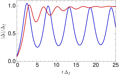
Figure 11: The order parameter versus time after the pairing strength was increased from $\Delta_{i}=0.05\Delta_{f}$ to $\Delta_{f}$ abruptly at $t=0$. The blue curve is for an isolated superconductor while the red curve is for a superconductor connected to leads. For this case a Thouless energy $E_{\rm Th}=0.075\Delta_{f}$ was used. The data was obtained using $501$ equally spaced levels with level spacing $\delta_{s}=0.02\Delta_{f}$. The capacitance was chosen $C=0.1e^{2}/\Delta_{f}$.

In our numerical implementation of the above, we work with the following parameters: The initial pairing interaction is such that for $t<0$, $\Delta=\Delta_{i}$. The increased pairing interaction strength corresponds to an equilibrium value of the order parameter $\Delta_{f}=20\Delta_{i}$. The persistent oscillations of $|\Delta(t)|$ in the isolated system are shown in the blue curve in Fig. 11. We repeat the calculation, now for a superconductor connected to leads. We use a s energy $E_{\rm Th}=0.075\Delta_{f}$. The result for $|\Delta(t)|$ in the presence of leads is the red curve in Fig. 11. We see that $|\Delta(t)|$ eventually decays to a constant, as expected. The extent of the damping is such that several oscillations are completed within the decay time. Hence we conclude that the numerical results that we obtained previously are outside the regime of overdamping. It follows that the lack of oscillatory behavior in Fig. 9 is due to the fact that the superconductor only gradually becomes aware of a change in the voltage.

V Conclusion

We have studied a voltage biased NISIN junction i.e. a superconducting island connected to normal leads by means of tunnel junctions. We restricted ourselves to the regime where the dominant energy relaxation mechanism in the superconductor is the tunneling of electrons from the superconductor to the leads. We also restricted ourselves to the regime of low transparency junctions where the position dependence of the order parameter inside the superconductor can be neglected.

In Sec. III we found the stationary states of the system. For these, the order parameter $\Delta$ and the chemical potential are implicitly determined by Eq. (35). We also found the current between the leads [cf. Eq. (36)]. The most striking feature of the stationary states is that there can be more than one stationary state at a given voltage. These are characterized by different values of $|\Delta|$ and of the current as can be seen in the $I$-$V$ curves of Fig. 7. Depending on system parameters, superconductivity can survive up to voltages large compared to $\Delta_{0}$, the order parameter of the isolated superconductor. In this case, increasing the voltage eventually leads to a second order phase transition to the normal state. We have found that the critical voltage at which the transition occurs obeys a power-law [cf. Eq. (40)].

In Sec. IV we studied time-dependent states of the system. In this way we were able to demonstrate the stability of the stationary states we have found in the previous section. Our results also indicate that a DC biased system always relaxes into a stationary state. In the parameter region of multiple stationary states we demonstrated bi-stability. Associated with this are first order phase-transitions: there are critical voltages where $\Delta$ (and the current) make finite jumps. Furthermore, there is hysteresis of $|\Delta|$ and the current associated with the bi-stability.

- (1) C. J. Lambert and R. Riamondi, J. Phys.: Condens. Matter 10, 901 (1998).
- (2) C. W. J. Beenakker, in Mesoscopic Quantum Physics, edited by E. Akkermans, G. Montambaux, J.-L. Pichard, and J. Zinn-Justin, (North-Holland, Amsterdam, 1995).
- (3) G. E. Blonder, M. Tinkham, and T. M. Klapwijk, Phys. Rev. B 25, 4515 (1982).
- (4) A. F. Andreev, Zh. Eksp. Teor. Fiz. 46, 1823 (1964), [Sov. Phys. JETP 19, 1228 (1964)].
- (5) B. D. Josephson, Phys. Lett. A 1, 251 (1962).
- (6) M. Tinkham, Introduction to superconductivity, (McGraw-Hill, New York, 1996).
- (7) N. B. Kopnin, Theory of Nonequilibrium Superconductivity, (Clarendon, Oxford, 2001).
- (8) R. A. Barankov and L. S. Levitov, Phys. Rev. Lett. 96, 230403 (2006); Phys. Rev. A 73 033614 (2006).
- (9) E. A. Yuzbashyan, B. L. Altshuler, V. B. Kuznetsov, and V. Z. Enolskii, J. Phys. A 38, 7831 (2005); Phys. Rev. B 72, 220503(R) (2005).
- (10) R. S. Keizer, M. G. Flokstra, J. Aarts, and T. M. Klapwijk, Phys. Rev. Lett. 96, 147002 (2006).
- (11) P. G. de Gennes, Superconductivity of Metals and Alloys, (Benjamin, New York, 1966).
- (12) I. U. Giaver, U.S. patent 116427 (1963).
- (13) M. Hidaka, S. Ishizaka, and J. Sone, J. Appl. Phys. 74, 7409 (1993).
- (14) J. Sánchez-Cañizares and F. Sols, J. Low Temp. Phys. 122, 11 (2001); J. Phys.: Condens. Matter 7, L317 (1995).
- (15) A. Martin and C. J. Lambert, Phys. Rev. B 51, 17999 (1995).
- (16) L. V. Keldysh, Zh. Eksp. Teor. Fiz. 47, 1515 (1964); [Sov. Phys. JETP 20, 1018 (1965)].
- (17) J. Rammer and H. Smith, Rev. Mod. Phys. 58, 323 (1986).
- (18) A. Brinkman, A. A. Golubov, H. Rogalla, F. K. Wilhelm, and M. Yu. Kupriyanov, Phys. Rev. B. 68, 224513 (2003).
- (19) Several different conventions exist for the definition of the Keldysh structure of the Green functions. Here we use the convention of Eqs. (2.26) and (2.27) in Ref. Ram86, .
- (20) W. Belzig, G. Schön, C. Bruder, and A. D. Zaikin, Superlattices Microstructures 25, 1251 (1999).
- (21) Yu. V. Nazarov, in: Handbook of Theoretical and Computational Nanotechnology, edited by M. Rieth and W. Schommers, (American Scientific Publishers, Stevenson Ranch, CA, 2006).
- (22) Yu. V. Nazarov, Superlattices Microstructures 25, 1221 (1999).
- (23) Yu. V. Nazarov, Phys. Rev. Lett. 73, 1420 (1994).
- (24) To derive this equation from the full theory as presented in Ref. Naz99, , the tunneling limit must be taken. This boils down to using Eq. (14) of Ref. Naz99, in stead of the more general Eq. (36).
- (25) A. L. Shelankov, J. Low Temp. Phys. 60, 29 (1985).
- (26) cf. Eqs. (36) and (37) of Ref. Naz99, .
- (27) While our numerical scheme breaks down when , it is again possible to do numerics when the system is perfectly isolated i.e. when is strictly zero.