Model-Based Compressive Sensing
Abstract
Compressive sensing (CS) is an alternative to Shannon/Nyquist sampling for the acquisition of sparse or compressible signals that can be well approximated by just elements from an -dimensional basis. Instead of taking periodic samples, CS measures inner products with random vectors and then recovers the signal via a sparsity-seeking optimization or greedy algorithm. Standard CS dictates that robust signal recovery is possible from measurements. It is possible to substantially decrease without sacrificing robustness by leveraging more realistic signal models that go beyond simple sparsity and compressibility by including structural dependencies between the values and locations of the signal coefficients. This paper introduces a model-based CS theory that parallels the conventional theory and provides concrete guidelines on how to create model-based recovery algorithms with provable performance guarantees. A highlight is the introduction of a new class of structured compressible signals along with a new sufficient condition for robust structured compressible signal recovery that we dub the restricted amplification property, which is the natural counterpart to the restricted isometry property of conventional CS. Two examples integrate two relevant signal models — wavelet trees and block sparsity — into two state-of-the-art CS recovery algorithms and prove that they offer robust recovery from just measurements. Extensive numerical simulations demonstrate the validity and applicability of our new theory and algorithms.
Index Terms:
Compressive sensing, sparsity, signal model, union of subspaces, wavelet tree, block sparsityI Introduction
We are in the midst of a digital revolution that is enabling the development and deployment of new sensors and sensing systems with ever increasing fidelity and resolution. The theoretical foundation is the Shannon/Nyquist sampling theorem, which states that a signal’s information is preserved if it is uniformly sampled at a rate at least two times faster than its Fourier bandwidth. Unfortunately, in many important and emerging applications, the resulting Nyquist rate can be so high that we end up with too many samples and must compress in order to store or transmit them. In other applications the cost of signal acquisition is prohibitive, either because of a high cost per sample, or because state-of-the-art samplers cannot achieve the high sampling rates required by Shannon/Nyquist. Examples include radar imaging and exotic imaging modalities outside visible wavelengths.
Transform compression systems reduce the effective dimensionality of an -dimensional signal by re-representing it in terms of a sparse or compressible set of coefficients in a basis expansion , with an basis matrix. By sparse we mean that only of the coefficients are nonzero and need to be stored or transmitted. By compressible we mean that the coefficients , when sorted, decay rapidly enough to zero that can be well-approximated as -sparse. The sparsity and compressibility properties are pervasive in many signal classes of interest. For example, smooth signals and images are compressible in the Fourier basis, while piecewise smooth signals and images are compressible in a wavelet basis [1]; the JPEG and JPEG2000 standards are examples of practical transform compression systems based on these bases.
Compressive sensing (CS) provides an alternative to Shannon/Nyquist sampling when the signal under acquisition is known to be sparse or compressible [2, 3, 4]. In CS, we measure not periodic signal samples but rather inner products with measurement vectors. In matrix notation, the measurements , where the rows of the matrix contain the measurement vectors. While the matrix is rank deficient, and hence loses information in general, it can be shown to preserve the information in sparse and compressible signals if it satisfies the so-called restricted isometry property (RIP) [3]. Intriguingly, a large class of random matrices have the RIP with high probability. To recover the signal from the compressive measurements , we search for the sparsest coefficient vector that agrees with the measurements. To date, research in CS has focused primarily on reducing both the number of measurements (as a function of and ) and on increasing the robustness and reducing the computational complexity of the recovery algorithm. Today’s state-of-the-art CS systems can robustly recover -sparse and compressible signals from just noisy measurements using polynomial-time optimization solvers or greedy algorithms.
While this represents significant progress from Nyquist-rate sampling, our contention in this paper is that it is possible to do even better by more fully leveraging concepts from state-of-the-art signal compression and processing algorithms. In many such algorithms, the key ingredient is a more realistic structured sparsity model that goes beyond simple sparsity by codifying the inter-dependency structure among the signal coefficients .111Obviously, sparsity and compressibility correspond to simple signal models where each coefficient is treated independently; for example in a sparse model, the fact that the coefficient is large has no bearing on the size of any , . We will reserve the use of the term “model” for situations where we are enforcing structured dependencies between the values and the locations of the coefficients . For instance, modern wavelet image coders exploit not only the fact that most of the wavelet coefficients of a natural image are small but also the fact that the values and locations of the large coefficients have a particular structure. Coding the coefficients according to a structured sparsity model enables these algorithms to compress images close to the maximum amount possible – significantly better than a naïve coder that just processes each large coefficient independently. We have previously developed a new CS recovery algorithm that promotes structure in the sparse representation by tailoring the recovered signal according to a sparsity-promoting probabilistic model, such as an Ising graphical model [5]. Such probabilistic models favor certain configurations for the magnitudes and indices of the significant coefficients of the signal.
In this paper, we expand on this concept by introducing a model-based CS theory that parallels the conventional theory and provides concrete guidelines on how to create structured signal recovery algorithms with provable performance guarantees. By reducing the number of degrees of freedom of a sparse/compressible signal by permitting only certain configurations of the large and zero/small coefficients, structured sparsity models provide two immediate benefits to CS. First, they enable us to reduce, in some cases significantly, the number of measurements required to stably recover a signal. Second, during signal recovery, they enable us to better differentiate true signal information from recovery artifacts, which leads to a more robust recovery.
To precisely quantify the benefits of model-based CS, we introduce and study several new theoretical concepts that could be of more general interest. We begin with structured sparsity models for -sparse signals and make precise how the structure reduces the number of potential sparse signal supports in . Then using the model-based restricted isometry property from [6, 7], we prove that such structured sparse signals can be robustly recovered from noisy compressive measurements. Moreover, we quantify the required number of measurements and show that for some structured sparsity models is independent of . These results unify and generalize the limited related work to date on structured sparsity models for strictly sparse signals [6, 7, 8, 9, 10]. We then introduce the notion of a structured compressible signal, whose coefficients are no longer strictly sparse but have a structured power-law decay. To establish that structured compressible signals can be robustly recovered from compressive measurements, we generalize the standard RIP to a new restricted amplification property (RAmP). Using the RAmP, we show that the required number of measurements for recovery of structured compressible signals is independent of .
To take practical advantage of this new theory, we demonstrate how to integrate structured sparsity models into two state-of-the-art CS recovery algorithms, CoSaMP [11] and iterative hard thresholding (IHT) [12, 13, 14, 15, 16]. The key modification is surprisingly simple: we merely replace the nonlinear sparse approximation step in these greedy algorithms with a structured sparse approximation. Thanks to our new theory, both new model-based recovery algorithms have provable robustness guarantees for both structured sparse and structured compressible signals.
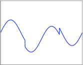
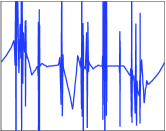
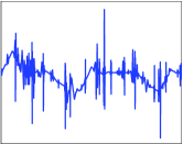
To validate our theory and algorithms and demonstrate their general applicability and utility, we present two specific instances of model-based CS and conduct a range of simulation experiments. The first structured sparsity model accounts for the fact that the large wavelet coefficients of piecewise smooth signals and images tend to live on a rooted, connected tree structure [17]. Using the fact that the number of such trees is much smaller than , the number of -sparse signal supports in dimensions, we prove that a tree-based CoSaMP algorithm needs only measurements to robustly recover tree-sparse and tree-compressible signals. This provides a significant reduction against the standard CS requirement as the signal length increases. Figure 1 indicates the potential performance gains on a tree-compressible, piecewise smooth signal.
 |
 |
 |
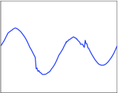 |
| (a) test signal | (b) CoSaMP | (c) -norm min. | (d) model-based recovery |
| (RMSE ) | (RMSE ) | (RMSE ) |
The second structured sparsity model accounts for the fact that the large coefficients of many sparse signals cluster together [8, 9]. Such a so-called block sparse model is equivalent to a joint sparsity model for an ensemble of , length- signals [10], where the supports of the signals’ large coefficients are shared across the ensemble. Using the fact that the number of clustered supports is much smaller than , we prove that a block-based CoSaMP algorithm needs only measurements to robustly recover block-sparse and block-compressible signals. In contrast, standard CS requires ; block sparsity reduces the dependence of on the signal length , particularly for large block sizes .
Our new theory and methods relate to a small body of previous work aimed at integrating structured sparsity into CS. Several groups have developed structured sparse signal recovery algorithms [6, 7, 8, 18, 19, 20, 21, 22, 23, 24]; however, their approaches have either been ad hoc or focused on a single structured sparsity model. Most previous work on unions of subspaces [6, 7, 24] has focused exclusively on strictly sparse signals and has considered neither compressibility nor feasible recovery algorithms. A related CS modeling framework for structured sparse and compressible signals [9] collects the samples of a signal into groups, , and allows signals where out of groups have nonzero coefficients. This framework is immediately applicable to block-sparse signals and signal ensembles with common sparse supports. While [9] provides recovery algorithms, measurement bounds, and recovery guarantees similar to those provided in Section VI, our proposed framework has the ability to focus on arbitrary subsets of the groups that yield more elaborate structures, such as connected subtrees for wavelet coefficients. To the best of our knowledge, our general algorithmic framework for model-based recovery, the concept of a model-compressible signal, and the associated RAmP are new to the literature.
This paper is organized as follows. A review of the CS theory in Section II lays out the foundational concepts that we extend to the model-based case in subsequent sections. Section III develops the concept of structured sparse signals and introduces the concept of structured compressible signals. We also quantify how structured sparsity models improve the measurement and recovery process by exploiting the model-based RIP for structured sparse signals and by introducing the RAmP for structured compressible signals. Section IV indicates how to tune CoSaMP to incorporate structured sparsity models and establishes its robustness properties for structured sparse and structured compressible signals; the modifications to the IHT algorithm are very similar, so we defer them to an appendix to reduce redundancy. Sections V and VI then specialize our theory to the special cases of wavelet tree and block sparse signal models, respectively, and report on a series of numerical experiments that validate our theoretical claims. We conclude with a discussion in Section VII. To make the paper more readable, all proofs are relegated to a series of appendices.
II Background on Compressive Sensing
II-A Sparse and compressible signals
Given a basis , we can represent every signal in terms of coefficients as ; stacking the as columns into the matrix , we can write succinctly that . In the sequel, we will assume without loss of generality that the signal is sparse or compressible in the canonical domain so that the sparsity basis is the identity and .
A signal is -sparse if only entries of are nonzero. We call the set of indices corresponding to the nonzero entries the support of and denote it by . The set of all -sparse signals is the union of the , -dimensional subspaces aligned with the coordinate axes in . We denote this union of subspaces by .
Many natural and manmade signals are not strictly sparse, but can be approximated as such; we call such signals compressible. Consider a signal whose coefficients, when sorted in order of decreasing magnitude, decay according to the power law
| (1) |
where indexes the sorted coefficients. Thanks to the rapid decay of their coefficients, such signals are well-approximated by -sparse signals. Let represent the best -term approximation of , which is obtained by keeping just the first terms in from (1). Denote the error of this approximation in the norm as
| (2) |
where the norm of the vector is defined as for . Then, for , we have that
| (3) |
with . That is, when measured in the norm, the signal’s best approximation error has a power-law decay with exponent as increases. In the sequel we let , yielding , and we dub a signal that obeys (3) an -compressible signal.
The approximation of compressible signals by sparse signals is the basis of transform coding as is used in algorithms like JPEG and JPEG2000 [1]. In this framework, we acquire the full -sample signal ; compute the complete set of transform coefficients via ; locate the largest coefficients and discard the smallest coefficients; and encode the values and locations of the largest coefficients. While a widely accepted standard, this sample-then-compress framework suffers from three inherent inefficiencies. First, we must start with a potentially large number of samples even if the ultimate desired is small. Second, the encoder must compute all of the transform coefficients , even though it will discard all but of them. Third, the encoder faces the overhead of encoding the locations of the large coefficients.
II-B Compressive measurements and the restricted isometry property
Compressive sensing (CS) integrates the signal acquisition and compression steps into a single process [2, 3, 4]. In CS we do not acquire directly but rather acquire linear measurements using an measurement matrix . We then recover by exploiting its sparsity or compressibility. Our goal is to push as close as possible to in order to perform as much signal “compression” during acquisition as possible.
In order to recover a good estimate of (the largest ’s, for example) from the compressive measurements, the measurement matrix should satisfy the restricted isometry property (RIP) [3].
Definition 1
An matrix has the -restricted isometry property (-RIP) with constant if, for all ,
| (4) |
In words, the -RIP ensures that all submatrices of of size are close to an isometry, and therefore distance (and information) preserving. Practical recovery algorithms typically require that have a slightly stronger -RIP, -RIP, or higher-order RIP in order to preserve distances between -sparse vectors (which are -sparse in general), three-way sums of -sparse vectors (which are -sparse in general), and other higher-order structures.
While checking whether a measurement matrix satisfies the -RIP is an NP-Complete problem in general [26], random matrices whose entries are independent and identically distributed (i.i.d.) Gaussian, Rademacher (), or more generally subgaussian222A random variable is called subgaussian if there exists such that for all . Examples include the Gaussian, Bernoulli, and Rademacher random variables, as well as any bounded random variable. [25] work with high probability provided . These random matrices also have a so-called universality property in that, for any choice of orthonormal basis matrix , has the -RIP with high probability. This is useful when the signal is sparse not in the canonical domain but in basis . A random corresponds to an intriguing data acquisition protocol in which each measurement is a randomly weighted linear combination of the entries of .
II-C Recovery algorithms
Since there are infinitely many signal coefficient vectors that produce the same set of compressive measurements , to recover the “right” signal we exploit our a priori knowledge of its sparsity or compressibility. For example, we could seek the sparsest that agrees with the measurements :
| (5) |
where the “norm” of a vector counts its number of nonzero entries. While this optimization can recover a -sparse signal from just compressive measurements, it is unfortunately a combinatorial, NP-hard problem [26]; furthermore, the recovery is not stable in the presence of noise [4].
Practical, stable recovery algorithms rely on the RIP (and therefore require at least measurements); they can be grouped into two camps. The first approach convexifies the “norm” minimization (5) to the -norm minimization
| (6) |
This corresponds to a linear program that can be solved in polynomial time [3, 2]. Adaptations to deal with additive noise in or include basis pursuit with denoising (BPDN) [27], complexity-based regularization [28], and the Dantzig Selector [29].
The second approach finds the sparsest agreeing with the measurements through an iterative, greedy search. Algorithms such as matching pursuit, orthogonal matching pursuit [30], StOMP [31], iterative hard thresholding (IHT) [12, 13, 14, 15, 16], CoSaMP [11], and Subspace Pursuit (SP) [32] all revolve around a best -term approximation for the estimated signal, with varying for each algorithm; typically is .
II-D Performance bounds on signal recovery
Given compressive measurements, a number of different CS signal recovery algorithms, including all of the -norm minimization techniques mentioned above and the CoSaMP, SP, and IHT iterative techniques, offer provably stable signal recovery with performance close to optimal -term approximation (recall (3)) [3, 2, 16, 11]. For a random , all results hold with high probability.
For a noise-free, -sparse signal, these algorithms offer perfect recovery, meaning that the signal recovered from the compressive measurements is exactly .
For a -sparse signal whose measurements are corrupted by noise of bounded norm (that is, we measure ) the mean-squared error of the signal is
| (7) |
with a small constant.
For an -compressible signal whose measurements are corrupted by noise of bounded norm, the mean-squared error of the recovered signal is
| (8) |
Using (3) we can simplify this expression to
| (9) |
For the recovery algorithm (6), we obtain a bound very similar to (8), albeit with the -norm error component removed [33].
III Structured Sparsity and Compressibility
While many natural and manmade signals and images can be described to first-order as sparse or compressible, the support of their large coefficients often has an underlying inter-dependency structure. This phenomenon has received only limited attention by the CS community to date [6, 7, 8, 9, 19, 20, 21, 22, 23]. In this section, we introduce a model-based theory of CS that captures such structure. A model reduces the degrees of freedom of a sparse/compressible signal by permitting only certain configurations of supports for the large coefficient. As we will show, this allows us to reduce, in some cases significantly, the number of compressive measurements required to stably recover a signal.
III-A Structured sparse signals
Recall from Section II-A that a -sparse signal vector lives in , which is a union of subspaces of dimension . Other than its -sparsity, there are no further constraints on the support or values of its coefficients. A structured sparsity model endows the -sparse signal with additional structure that allows certain -dimensional subspaces in and disallows others [6, 7].
To state a formal definition of a structured sparsity model, let represent the entries of corresponding to the set of indices , and let denote the complement of the set .
Definition 2
A structured sparsity model is defined as the union of canonical -dimensional subspaces
where is the set containing all allowed supports, with for each , and each subspace contains all signals with .
Signals from are called -structured sparse. Clearly, and contains subspaces.
In Sections V and VI below we consider two concrete structured sparsity models. The first model accounts for the fact that the large wavelet coefficients of piecewise smooth signals and images tend to live on a rooted, connected tree structure [17]. The second model accounts for the fact that the large coefficients of sparse signals often cluster together into blocks [8, 9, 10].
III-B Model-based RIP
If we know that the signal being acquired is -structured sparse, then we can relax the RIP constraint on the CS measurement matrix and still achieve stable recovery from the compressive measurements [6, 7].
Definition 3
Blumensath and Davies [6] have quantified the number of measurements necessary for a random CS matrix to have the -RIP with a given probability.
Theorem 1
[6] Let be the union of subspaces of -dimensions in . Then, for any and any
where is a positive constant, an i.i.d. subgaussian random matrix has the -RIP with constant with probability at least .
This bound can be used to recover the conventional CS result by substituting . Similarly, as the number of subspaces that arise from the structure imposed can be significantly smaller than the standard , the number of rows needed for a random matrix to have the -RIP can be significantly lower than the number of rows needed for the standard RIP. The -RIP property is sufficient for robust recovery of structured sparse signals, as we show below in Section IV-B.
III-C Structured compressible signals
Just as compressible signals are “nearly -sparse” and thus live close to the union of subspaces in , structured compressible signals are “nearly -structured sparse” and live close to the restricted union of subspaces . In this section, we make this new concept rigorous. Recall from (3) that we defined compressible signals in terms of the decay of their -term approximation error.
The error incurred by approximating by the best structured sparse approximation in is given by
We define as the algorithm that obtains the best -term structured sparse approximation of in the union of subspaces :
This implies that . The decay of this approximation error defines the structured compressibility of a signal.
Definition 4
The set of -structured compressible signals is defined as
Define as the smallest value of for which this condition holds for and .
We say that is an -structured compressible signal under the structured sparsity model . These approximation classes have been characterized for certain structured sparsity models; see Section V for an example. We will select the value of for which the distance between the approximation errors and the corresponding bounds is minimal.
III-D Nested model approximations and residual subspaces
In conventional CS, the same requirement (RIP) is a sufficient condition for the stable recovery of both sparse and compressible signals. In model-based recovery, however, the class of structured compressible signals is much larger than that of structured sparse signals, since the union of subspaces defined by structured sparse signals does not contain all canonical -dimensional subspaces.
To address this difference, we introduce some additional tools to develop a sufficient condition for the stable recovery of structured compressible signals. We will pay particular attention to structured sparsity models that generate nested approximations, since they are more amenable to analysis and computation.
Definition 5
A structured sparsity model has the nested approximation property (NAP) if for all and for all .
In words, a structured sparsity model generates nested approximations if the support of the best -term structured sparse approximation contains the support of the best -term structured sparse approximation for all . An important example of a NAP-generating structured sparse model is the standard compressible signal model of (3).
When a structured sparsity model obeys the NAP, the support of the difference between the best -term structured sparse approximation and the best -term structured sparse approximation of a signal can be shown to lie in a small union of subspaces, thanks to the structure enforced by the model. This structure is captured by the set of subspaces that are included in each subsequent approximation, as defined below.
Definition 6
The set of residual subspaces of size is defined as , for .
Under the NAP, each structured compressible signal can be partitioned into its best -term structured sparse approximation , the additional components present in the best -term structured sparse approximation , and so on, with and for each . Each signal partition is a -sparse signal, and thus is a union of subspaces of dimension . We will denote by the number of subspaces that compose and omit the dependence on in the sequel for brevity.
Intuitively, the norms of the partitions decay as increases for signals that are structured compressible. As the next subsection shows, this observation is instrumental in relaxing the isometry restrictions on the measurement matrix and bounding the recovery error for -structured compressible signals when the model obeys the NAP.
III-E The restricted amplification property (RAmP)
For exactly -structured sparse signals, we discussed in Section III-B that the number of compressive measurements required for a random matrix to have the -RIP is determined by the number of canonical subspaces via (1). Unfortunately, such structured sparse concepts and results do not immediately extend to structured compressible signals. Thus, we develop a generalization of the -RIP that we will use to quantify the stability of recovery for structured compressible signals.
One way to analyze the robustness of compressible signal recovery in conventional CS is to consider the tail of the signal outside its -term approximation as contributing additional “noise” to the measurements of size [33, 11, 16]. Consequently, the conventional -sparse recovery performance result can be applied with the augmented noise .
This technique can also be used to quantify the robustness of structured compressible signal recovery. The key quantity we must control is the amplification of the structured sparse approximation residual through . The following property is a new generalization of the RIP and model-based RIP.
Definition 7
A matrix has the -restricted amplification property (RAmP) for the residual subspaces of model if
| (11) |
for any for each .
The regularity parameter caps the growth rate of the amplification of as a function of . Its value can be chosen so that the growth in amplification with balances the decay of the norm in each residual subspace with .
We can quantify the number of compressive measurements required for a random measurement matrix to have the RAmP with high probability; we prove the following in Appendix A.
Theorem 2
Let be an matrix with i.i.d. subgaussian entries and let the set of residual subspaces of the structured sparsity model contain subspaces of dimension for each . If
| (12) |
then the matrix has the -RAmP with probability .
The order of the bound of Theorem 2 is lower than as long as the number of subspaces grows slower than .
Armed with the RaMP, we can state the following result, which will provide robustness for the recovery of structured compressible signals; see Appendix B for the proof.
Theorem 3
Let be an -structured compressible signal under a structured sparsity model that obeys the NAP. If has the -RAmP and , then we have
where is a constant that depends only on .
IV Model-Based Signal Recovery Algorithms
To take practical advantage of our new theory for model-based CS, we demonstrate how to integrate structured sparsity models into two state-of-the-art CS recovery algorithms, CoSaMP [11] (in this section) and iterative hard thresholding (IHT) [12, 13, 14, 15, 16] (in Appendix C to avoid repetition). The key modification is simple: we merely replace the best -term sparse approximation step in these greedy algorithms with a best -term structured sparse approximation. Since at each iteration we need only search over the subspaces of rather than subspaces of , fewer measurements will be required for the same degree of robust signal recovery. Or, alternatively, using the same number of measurements, more accurate recovery can be achieved.
After presenting the modified CoSaMP algorithm, we prove robustness guarantees for both structured sparse and structured compressible signals. To this end, we must define an enlarged union of subspaces that includes sums of elements in the structured sparsity model.
Definition 8
The -order sum for the set , with an integer, is defined as
Define as the algorithm that obtains the best approximation of in the enlarged union of subspaces :
We note that . Note also that for many structured sparsity models, we will have , and so the algorithm will provide a strictly better approximation than .
IV-A Model-based CoSaMP
We choose to modify the CoSaMP algorithm [11] for two reasons. First, it has robust recovery guarantees that are on par with the best convex optimization-based approaches. Second, it has a simple iterative, greedy structure based on a best -term approximation (with a small integer) that is easily modified to incorporate a best -term structured sparse approximation . These properties also make the IHT and SP algorithms amenable to modification; see Appendix C for details on IHT. Pseudocode for the modified CoSaMP algorithm is given in Algorithm 1, where denotes the Moore-Penrose pseudoinverse of .
| Inputs: CS matrix , measurements , structured sparse approximation algorithm | ||
| Output: -sparse approximation to true signal | ||
| , ; {initialize} | ||
| while | halting criterion false do | |
| 1. | ||
| 2. | {form signal residual estimate} | |
| 3. | {prune residual estimate according to structure} | |
| 4. | {merge supports} | |
| 5. , | {form signal estimate} | |
| 6. | {prune signal estimate according to structure} | |
| 7. | {update measurement residual} | |
| end while | ||
| return |
IV-B Performance of structured sparse signal recovery
We now study the performance of model-based CoSaMP signal recovery on structured sparse and structured compressible signals. A robustness guarantee for noisy measurements of structured sparse signals can be obtained using the model-based RIP (10). Our performance guarantee for structured sparse signal recovery will require that the measurement matrix be a near-isometry for all subspaces in for some . This requirement is a direct generalization of the -RIP, -RIP, and higher-order RIPs from the conventional CS theory. The following theorem is proven in Appendix D.
Theorem 4
Let and let be a set of noisy CS measurements. If has an -RIP constant of , then the signal estimate obtained from iteration of the model-based CoSaMP algorithm satisfies
| (13) |
This guarantee matches that of the CoSaMP algorithm [11, Theorem 4.1]; however, our guarantee is only for structured sparse signals rather than for all sparse signals.
IV-C Performance of structured compressible signal recovery
Using the new tools introduced in Section III, we can provide a robustness guarantee for noisy measurements of structured compressible signals, using the RAmP as a condition on the measurement matrix .
Theorem 5
Let be an -structured compressible signal from a structured sparsity model that obeys the NAP, and let be a set of noisy CS measurements. If has the -RIP with and the -RAmP with and , then the signal estimate obtained from iteration of the model-based CoSaMP algorithm satisfies
| (14) | |||||
Proof sketch. To prove the theorem, we first bound the optimal structured sparse recovery error for an -structured compressible signal when the matrix has the -RAmP with (see Theorem 3). Then, using Theorem 13, we can easily prove the result by following the analogous proof in [11]. ∎
The standard CoSaMP algorithm also features a similar guarantee for structured compressible signals, with the constant changing from 35 to 20.
IV-D Robustness to model mismatch
We now analyze the robustness of model-based CS recovery to model mismatch, which occurs when the signal being recovered from compressive measurements does not conform exactly to the structured sparsity model used in the recovery algorithm.
We begin with optimistic results for signals that are “close” to matching the recovery structured sparsity model. First consider a signal that is not -structured sparse as the recovery algorithm assumes but rather -structured sparse for some small integer . This signal can be decomposed into , the signal’s -term structured sparse approximation, and , the error of this approximation. For , we have that . If the matrix has the -RAmP, then it follows than
| (15) |
Using equations (13) and (15), we obtain the following guarantee for the iteration of model-based CoSaMP:
By noting that is small, we obtain a guarantee that is close to (13).
Second, consider a signal that is not -structured compressible as the recovery algorithm assumes but rather -structured compressible. The following bound can be obtained under the conditions of Theorem 5 by modifying the argument in Appendix B:
As becomes smaller, the factor approaches , matching (14). In summary, as long as the deviations from the structured sparse and structured compressible classes are small, our model-based recovery guarantees still apply within a small bounded constant factor.
We end with an intuitive worst-case result for signals that are arbitrarily far away from structured sparse or structured compressible. Consider such an arbitrary and compute its nested structured sparse approximations , . If is not structured compressible, then the structured sparse approximation error is not guaranteed to decay as decreases. Additionally, the number of residual subspaces could be as large as ; that is, the difference between subsequent structured sparse approximations might lie in any arbitrary -dimensional subspace. This worst case is equivalent to setting and in Theorem 2. It is easy to see that the resulting condition on the number of measurements matches that of the standard RIP for CS. Hence, if we inflate the number of measurements to (the usual number for conventional CS), the performance of model-based CoSaMP recovery on an arbitrary signal follows the distortion of the best -term structured sparse approximation error of within a bounded constant factor.
IV-E Computational complexity of model-based recovery
The computational complexity of a structured signal recovery algorithm differs from that of a standard algorithm by two factors. The first factor is the reduction in the number of measurements necessary for recovery: since most current recovery algorithms have a computational complexity that is linear in the number of measurements, any reduction in reduces the total complexity. The second factor is the cost of the structured sparse approximation. The -term approximation used in most current recovery algorithms can be implemented with a simple sorting operation ( complexity, in general). Ideally, the structured sparsity model should support a similarly efficient approximation algorithm.
To validate our theory and algorithms and demonstrate their general applicability and utility, we now present two specific instances of model-based CS and conduct a range of simulation experiments.
V Example: Wavelet Tree Model
Wavelet decompositions have found wide application in the analysis, processing, and compression of smooth and piecewise smooth signals because these signals are -sparse and compressible, respectively [1]. Moreover, the wavelet coefficients can be naturally organized into a tree structure, and for many kinds of natural and manmade signals the largest coefficients cluster along the branches of this tree. This motivates a connected tree model for the wavelet coefficients [34, 35, 36].
While CS recovery for wavelet-sparse signals has been considered previously [19, 20, 21, 22, 23], the resulting algorithms integrated the tree constraint in an ad-hoc fashion. Furthermore, the algorithms provide no recovery guarantees or bounds on the necessary number of compressive measurements.
V-A Tree-sparse signals
We first describe tree sparsity in the context of sparse wavelet decompositions. We focus on one-dimensional signals and binary wavelet trees, but all of our results extend directly to -dimensional signals and -ary wavelet trees.
Consider a signal of length , for an integer value of . The wavelet representation of is given by
where is the scaling function and is the wavelet function at scale and offset . The wavelet transform consists of the scaling coefficient and wavelet coefficients at scale , , and position , . In terms of our earlier matrix notation, has the representation , where is a matrix containing the scaling and wavelet functions as columns, and is the vector of scaling and wavelet coefficients. We are, of course, interested in sparse and compressible .
The nested supports of the wavelets at different scales create a parent/child relationship between wavelet coefficients at different scales. We say that is the parent of and that and are the children of . These relationships can be expressed graphically by the wavelet coefficient tree in Figure 2.
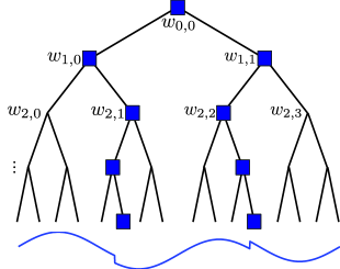
Wavelet functions act as local discontinuity detectors, and using the nested support property of wavelets at different scales, it is straightforward to see that a signal discontinuity will give rise to a chain of large wavelet coefficients along a branch of the wavelet tree from a leaf to the root. Moreover, smooth signal regions will give rise to regions of small wavelet coefficients. This “connected tree” property has been well-exploited in a number of wavelet-based processing [17, 37, 38] and compression [39, 40] algorithms. In this section, we will specialize the theory developed in Sections III and IV to a connected tree model .
A set of wavelet coefficients forms a connected subtree if, whenever a coefficient , then its parent as well. Each such set defines a subspace of signals whose support is contained in ; that is, all wavelet coefficients outside are zero. In this way, we define the structured sparsity model as the union of all -dimensional subspaces corresponding to supports that form connected subtrees.
Definition 9
Define the set of -tree sparse signals as
To quantify the number of subspaces in , it suffices to count the number of distinct connected subtrees of size in a binary tree of size . We prove the following result in Appendix E.
Proposition 1
The number of subspaces in obeys for and for .
To simplify the presentation in the sequel, we will simply use the weaker bound for all values of and .
V-B Tree-based approximation
To implement tree-based signal recovery, we seek an efficient algorithm to solve the optimal approximation
| (16) |
Fortuitously, an efficient solver exists, called the condensing sort and select algorithm (CSSA) [34, 35, 36]. Recall that subtree approximation coincides with standard -term approximation (and hence can be solved by simply sorting the wavelet coefficients) when the wavelet coefficients are monotonically nonincreasing along the tree branches out from the root. The CSSA solves (16) in the case of general wavelet coefficient values by condensing the nonmonotonic segments of the tree branches using an iterative sort-and-average routine during a greedy search through the nodes. For each node in the tree, the algorithm calculates the average wavelet coefficient magnitude for each subtree rooted at that node, and records the largest average among all the subtrees as the energy for that node. The CSSA then searches for the unselected node with the largest energy and adds the subtree corresponding to the node’s energy to the estimated support as a supernode: a single node that provides a condensed representation of the corresponding subtree [36]. Condensing a large coefficient far down the tree accounts for the potentially large cost (in terms of the total budget of tree nodes ) of growing the tree to that point.
Since the first step of the CSSA involves sorting all of the wavelet coefficients, overall it requires computations. However, once the CSSA grows the optimal tree of size , it is trivial to determine the optimal trees of size and computationally efficient to grow the optimal trees of size [34].
The constrained optimization (16) can be rewritten as an unconstrained problem by introducing the Lagrange multiplier [41]:
where and are the wavelet coefficients of . Except for the inconsequential term, this optimization coincides with Donoho’s complexity penalized sum of squares [41], which can be solved in only computations using coarse-to-fine dynamic programming on the tree. Its primary shortcoming is the nonobvious relationship between the tuning parameter and and the resulting size of the optimal connected subtree.
V-C Tree-compressible signals
Definition 10
Define the set of -tree compressible signals as
Furthermore, define as the smallest value of for which this condition holds for and .
Tree approximation classes contain signals whose wavelet coefficients have a loose (and possibly interrupted) decay from coarse to fine scales. These classes have been well-characterized for wavelet-sparse signals [40, 36, 35] and are intrinsically linked with the Besov spaces . Besov spaces contain functions of one or more continuous variables that have (roughly speaking) derivatives in ; the parameter provides finer distinctions of smoothness. When a Besov space signal with is sampled uniformly and converted to a length- vector , its wavelet coefficients belong to the tree approximation space , with
where “” denotes an equivalent norm. The same result holds if and .
V-D Stable tree-based recovery from compressive measurements
For tree-sparse signals, by applying Theorem 1 and Proposition 1, we find that a subgaussian random matrix has the -RIP property with constant and probability if the number of measurements obeys
Thus, the number of measurements necessary for stable recovery of tree-sparse signals is linear in , without the dependence on present in conventional non-model-based CS recovery.
For tree-compressible signals, we must quantify the number of subspaces in each residual set for the approximation class. We can then apply the theory of Section IV-C with Proposition 1 to calculate the smallest allowable via Theorem 5.
Proposition 2
The number of -dimensional subspaces that comprise obeys
| (17) |
Using Proposition 17 and Theorem 5, we obtain the following condition for the matrix to have the RAmP, which is proved in Appendix F.
Proposition 3
Let be an matrix with i.i.d. subgaussian entries. If
then the matrix has the -RAmP for the structured sparsity model and all with probability .
V-E Experiments
We now present the results of a number of numerical experiments that illustrate the effectiveness of a tree-based recovery algorithm. Our consistent observation is that explicit incorporation of the structured sparsity model in the recovery process significantly improves the quality of recovery for a given number of measurements. In addition, model-based recovery remains stable when the inputs are no longer tree-sparse, but rather are tree-compressible and/or corrupted with differing levels of noise. We employ the Daubechies-6 wavelet basis for sparsity, and recover the signal using model-based CoSaMP (Algorithm 1) with a CSSA-based structured sparse approximation step in all experiments.
We first study one-dimensional signals that match the connected wavelet-tree model described above. Among such signals is the class of piecewise smooth functions, which are commonly encountered in analysis and practice.
Figure 1 illustrates the results of recovering the tree-compressible HeaviSine signal of length from noise-free random Gaussian measurements using CoSaMP, -norm minimization using the l1_eq solver from the -Magic toolbox,333http://www.acm.caltech.edu/l1magic. and our tree-based recovery algorithm. It is clear that the number of measurements () is far fewer than the minimum number required by CoSaMP and -norm minimization to accurately recover the signal. In contrast, tree-based recovery using is accurate and uses fewer iterations to converge than conventional CoSaMP. Moreover, the normalized magnitude of the squared error for tree-based recovery is equal to 0.037, which is remarkably close to the error between the noise-free signal and its best -term tree-approximation (0.036).
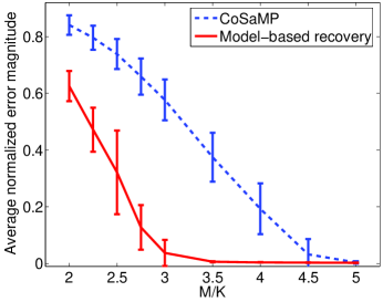
Figure 3(a) illustrates the results of a Monte Carlo simulation study on the impact of the number of measurements on the performance of model-based and conventional recovery for a class of tree-sparse piecewise polynomial signals. Each data point was obtained by measuring the normalized recovery error of 500 sample trials. Each sample trial was conducted by generating a new piecewise polynomial signal of length with five polynomial pieces of cubic degree and randomly placed discontinuities, computing its best -term tree-approximation using the CSSA, and then measuring the resulting signal using a matrix with i.i.d. Gaussian entries. Model-based recovery attains near-perfect recovery at measurements, while CoSaMP only matches this performance at .
 |
 |
| (a) | (b) |
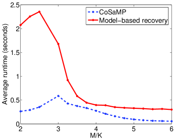
For the same class of signals, we empirically compared the recovery times of our proposed algorithm with those of the standard approach (CoSaMP). Experiments were conducted on a Sun workstation with a 1.8GHz AMD Opteron dual-core processor and 2GB memory running UNIX, using non-optimized Matlab code and a function-handle based implementation of the random projection operator . As is evident from Figure 3(b), wavelet tree-based recovery is in general slower than CoSaMP. This is due to the fact that the CSSA step in the iterative procedure is more computationally demanding than simple term approximation. Nevertheless, the highest benefits of model-based CS recovery are obtained around ; in this regime, the runtimes of the two approaches are comparable, with tree-based recovery requiring fewer iterations and yielding much smaller recovery error than standard recovery.
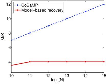
Figure 4 shows the growth of the overmeasuring factor with the signal length for conventional CS and model-based recovery. We generated 50 sample piecewise cubic signals and numerically computed the minimum number of measurements required for the recovery error , the best tree-approximation error, for every sample signal. The figure shows that while doubling the signal length increases the number of measurements required by standard recovery by , the number of measurements required by model-based recovery is constant for all . These experimental results verify the theoretical performance described in Proposition 3.
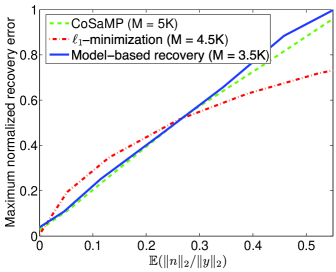
Further, we demonstrate that model-based recovery performs stably in the presence of measurement noise. We generated sample piecewise polynomial signals as above, computed their best -term tree-approximations, computed measurements of each approximation, and finally added Gaussian noise of variance to each measurement, so that the expected variance . We emphasize that this noise model implies that the energy of the noise added will be larger as increases. Then, we recovered the signals using CoSaMP and model-based recovery and measured the recovery error in each case. For comparison purposes, we also tested the recovery performance of a -norm minimization algorithm that accounts for the presence of noise, which has been implemented as the l1_qc solver in the -Magic toolbox. First, we determined the lowest value of for which the respective algorithms provided near-perfect recovery in the absence of noise in the measurements. This corresponds to for model-based recovery, for CoSaMP, and for -norm minimization. Next, we generated 200 sample tree-structured signals, computed noisy measurements, recovered the signal using the given algorithm and recorded the recovery error. Figure 5 illustrates the growth in maximum normalized recovery error (over the 200 sample trials) as a function of the expected measurement signal-to-noise ratio for the tree algorithms. We observe similar stability curves for all three algorithms, while noting that model-based recovery offers this kind of stability using significantly fewer measurements.
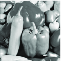
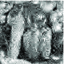
Finally, we turn to two-dimensional images and a wavelet quadtree model. The connected wavelet-tree model has proven useful for compressing natural images [35]; thus, our algorithm provides a simple and provably efficient method for recovering a wide variety of natural images from compressive measurements. An example of recovery performance is given in Figure 6. The test image (Peppers) is of size pixels, and we computed random Gaussian measurements. Model-based recovery again offers higher performance than standard signal recovery algorithms like CoSaMP, both in terms of recovery mean-squared error and visual quality.
 |
 |
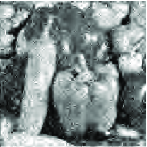 |
| (a) Peppers | (b) CoSaMP | (c) model-based rec. |
| (RMSE ) | (RMSE ) |
VI Example: Block-Sparse Signals and Signal Ensembles
In a block-sparse signal, the locations of the significant coefficients cluster in blocks under a specific sorting order. Block-sparse signals have been previously studied in CS applications, including DNA microarrays and magnetoencephalography [8, 9]. An equivalent problem arises in CS for signal ensembles, such as sensor networks and MIMO communication [10, 42, 9]. In this case, several signals share a common coefficient support set. For example, when a frequency-sparse acoustic signal is recorded by an array of microphones, then all of the recorded signals contain the same Fourier frequencies but with different amplitudes and delays. Such a signal ensemble can be re-shaped as a single vector by concatenation, and then the coefficients can be rearranged so that the concatenated vector exhibits block sparsity.
It has been shown that the block-sparse structure enables signal recovery from a reduced number of CS measurements, both for the single signal case [8, 9, 43] and the signal ensemble case [10], through the use of specially tailored recovery algorithms. However, the robustness guarantees for the algorithms [8, 43] either are restricted to exactly sparse signals and noiseless measurements, do not have explicit bounds on the number of necessary measurements, or are asymptotic in nature. An optimization-based algorithm introduced in [9] provides similar recovery guarantees to those obtained by the algorithm we present in this chapter; thus, our method can be interpreted as a greedy-based counterpart to that provided in [9].
In this section, we formulate the block sparsity model as a union of subspaces and pose an approximation algorithm on this union of subspaces. The approximation algorithm is used to implement block-based signal recovery. We also define the corresponding class of block-compressible signals and quantify the number of measurements necessary for robust recovery.
VI-A Block-sparse signals
Consider a class of signal vectors , with and integers. This signal can be reshaped into a matrix , and we use both notations interchangeably in the sequel. We will restrict entire columns of to be part of the support of the signal as a group. That is, signals in a block-sparse model have entire columns as zeros or nonzeros. The measure of sparsity for is its number of nonzero columns. More formally, we make the following definition.
It is important to note that a -block sparse signal has sparsity , which is dependent on the size of the block . We can extend this formulation to ensembles of , length- signals with common support. Denote this signal ensemble by , with , . We formulate a matrix representation of the ensemble that features the signal in its row: . The matrix features the same structure as the matrix obtained from a block-sparse signal; thus, the matrix can be converted into a block-sparse vector that represents the signal ensemble.
VI-B Block-based approximation
To pose the block-based approximation algorithm, we need to define the mixed norm of a matrix.
Definition 12
The mixed norm of the matrix is defined as
When , simply counts the number of nonzero columns in .
We immediately find that , with the vectorization of . Intuitively, we pose the algorithm to obtain the best block-based approximation of the signal as follows:
| (18) |
It is easy to show that to obtain the approximation, it suffices to perform column-wise hard thresholding: let be the largest -norm among the columns of . Then our approximation algorithm is , where
for each . Alternatively, a recursive approximation algorithm can be obtained by sorting the columns of by their norms, and then selecting the columns with largest norms. The complexity of this sorting process is .
VI-C Block-compressible signals
The approximation class under the block-compressible model corresponds to signals with blocks whose norm has a power-law decay rate.
Definition 13
We define the set of -block compressible signals as
where indexes the sorted column norms.
We say that is an -block compressible signal if . For such signals, we have , and . Note that the block-compressible model does not impart a structure to the decay of the signal coefficients, so that the sets are equal for all values of ; due to this property, the -RAmP is implied by the -RIP. Taking this into account, we can derive the following result from [11], which is proven similarly to Theorem 13.
Theorem 6
Let be a signal from the structured sparsity model , and let be a set of noisy CS measurements. If has the -RIP with , then the estimate obtained from iteration of block-based CoSaMP, using the approximation algorithm (18), satisfies
Thus, the algorithm provides a recovered signal of similar quality to approximations of by a small number of nonzero columns. When the signal is -block sparse, we have that , obtaining the same result as Theorem 13, save for a constant factor.
VI-D Stable block-based recovery from compressive measurements
Since Theorem 6 poses the same requirement on the measurement matrix for sparse and compressible signals, the same number of measurements is required to provide performance guarantees for block-sparse and block-compressible signals. The class contains subspaces of dimension . Thus, a subgaussian random matrix has the -RIP property with constant and probability if the number of measurements obeys
| (19) |
To compare with the standard CS measurement bound, the number of measurements required for robust recovery scales as , which is a substantial improvement over the that would be required by conventional CS recovery methods. When the size of the block is larger than , then this term becomes ; that is, it is linear on the total sparsity of the block-sparse signal.
We note in passing that the bound on the number of measurements (19) assumes a dense subgaussian measurement matrix, while the measurement matrices used in [10] have a block-diagonal structure. To obtain measurements from an dense matrix in a distributed setting, it suffices to partition the matrix into pieces of size and calculate the CS measurements at each sensor with the corresponding matrix; these individual measurements are then summed to obtain the complete measurement vector. For large , (19) implies that the total number of measurements required for recovery of the signal ensemble is lower than the bound for the case where each signal recovery is performed independently for each signal ().
VI-E Experiments
We conducted several numerical experiments comparing model-based recovery to CoSaMP in the context of block-sparse signals. We employ the model-based CoSaMP recovery of Algorithm 1 with the block-based approximation algorithm (18) in all cases. For brevity, we exclude a thorough comparison of our model-based algorithm with -norm minimization and defer it to future work. In practice, we observed that our algorithm performs several times faster than convex optimization-based procedures.
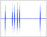
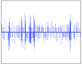
Figure 7 illustrates an signal that exhibits block sparsity, and its recovered version from measurements using CoSaMP and model-based recovery. The block size and there were active blocks in the signal. We observe the clear advantage of using the block-sparsity model in signal recovery.
 |
 |
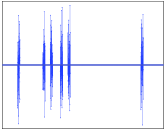 |
| (a) original block-sparse signal | (b) CoSaMP | (c) model-based recovery |
| (RMSE ) | (RMSE ) |
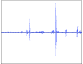
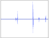
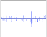
We now consider block-compressible signals. An example recovery is illustrated in Figure 8. In this case, the -norms of the blocks decay according to a power law, as described above. Again, the number of measurements is far below the minimum number required to guarantee stable recovery through conventional CS recovery. However, enforcing the structured sparsity model in the approximation process results in a solution that is very close to the best 5-block approximation of the signal.
 |
 |
 |
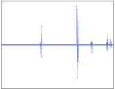 |
| (a) signal | (b) best 5-block approximation | (c) CoSaMP | (d) model-based recovery |
| (RMSE ) | (RMSE ) | (RMSE ) |
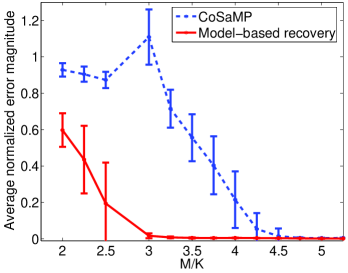
Figure 9(a) indicates the decay in recovery error as a function of the numbers of measurements for CoSaMP and model-based recovery. We generated sample block-sparse signals as follows: we randomly selected a set of blocks, each of size , and endow them with coefficients that follow an i.i.d. Gaussian distribution. Each sample point in the curves is generated by performing 200 trials of the corresponding algorithm. As in the connected wavelet-tree case, we observe clear gains using model-based recovery, particularly for low-measurement regimes; CoSaMP matches model-based recovery only for
 |
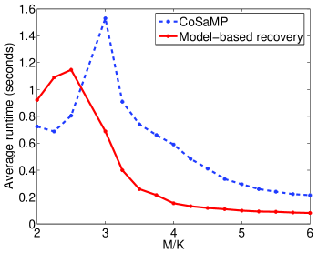 |
| (a) | (b) |
Figure 9(b) compares the recovery times of the two approaches. For this particular model, we observe that our proposed approach is in general much faster than CoSaMP. This is because of two reasons: a) the block-based approximation step involves sorting fewer coefficients, and thus is faster than term approximation; b) block-based recovery requires fewer iterations to converge to the true solution.
VII Conclusions
In this paper, we have aimed to demonstrate that there are significant performance gains to be made by exploiting more realistic and richer signal models beyond the simplistic sparse and compressible models that dominate the CS literature. Building on the unions of subspaces results of [6] and the proof machinery of [11], we have taken some first steps towards what promises to be a general theory for model-based CS by introducing the notion of a structured compressible signal and the associated restricted amplification property (RAmP) condition it imposes on the measurement matrix . Our analysis poses the nested approximation property (NAP) as a sufficient condition that is satisfied by many structured sparsity models.
For the volumes of natural and manmade signals and images that are wavelet-sparse or compressible, our tree-based CoSaMP and IHT algorithms offer performance that significantly exceeds today’s state-of-the-art while requiring only rather than random measurements. For block-sparse signals and signal ensembles with common sparse support, our block-based CoSaMP and IHT algorithms offer not only excellent performance but also require just measurements, where is the signal sparsity. Furthermore, block-based recovery can recover signal ensembles using fewer measurements than the number required when each signal is recovered independently; we have shown such advantages using real-world data from environmental sensor networks [44]. Additional structured sparsity models have been developed using our general framework in [45] and [46]; we have also released a Matlab toolbox containing the corresponding model-based CS recovery algorithms, available at http://dsp.rice.edu/software.
There are many avenues for future work on model-based CS. We have only considered the recovery of signals from models that can be geometrically described as a union of subspaces; possible extensions include other, more complex geometries such as high-dimensional polytopes and nonlinear manifolds. We also expect that the core of our proposed algorithms — a structured sparse approximation step — can be integrated into other iterative algorithms, such as relaxed -norm minimization methods. Furthermore, our framework will benefit from the formulation of new structured sparsity models that are endowed with efficient structured sparse approximation algorithms.
Appendix A Proof of Theorem 2
To prove this theorem, we will study the distribution of the maximum singular value of a submatrix of a matrix with i.i.d. Gaussian entries corresponding to the columns indexed by . From this we obtain the probability that RAmP does not hold for a fixed support . We will then evaluate the same probability for all supports of elements of , where the desired bound on the amplification is dependent on the value of . This gives us the probability that the RAmP does not hold for a given residual subspace set . We fix the probability of failure on each of these sets; we then obtain probability that the matrix does not have the RAmP using a union bound. We end by obtaining conditions on the number of rows of to obtain a desired probability of failure.
We begin from the following concentration of measure for the largest singular value of a submatrix , , of an matrix with i.i.d. subgaussian entries that are properly normalized [47, 48, 25]:
For large enough , ; thus we ignore this small constant in the sequel. By letting (with the appropriate value of for ), we obtain
We use a union bound over all possible supports for to obtain the probability that amplifies the norm of some by more than :
Bound the right hand side by a constant ; this requires
| (20) |
for each . We use another union bound among the residual subspaces to measure the probability that the RAmP does not hold:
To bound this probability by , we need ; plugging this into (20), we obtain
for each . Simplifying, we obtain that for to posess the RAmP with probability , the following must hold for all :
| (21) |
Since for , then the hypothesis (12) implies (21), proving the theorem. ∎
Appendix B Proof of Theorem 3
In this proof, we denote for brevity. To bound we write as
where
is the difference between the best structured sparse approximation and the best structured sparse approximation. Additionally, each piece . Therefore, since satisfies the -RAmP, we obtain
Since , the norm of each piece can be bounded as
Applying this bound in (B), we obtain
It is easy to show, using Euler-Maclaurin summations, that ; we then obtain
which proves the theorem. ∎
Appendix C Model-based Iterative Hard Thresholding
Our proposed model-based iterative hard thresholding (IHT) is given in Algorithm 2. For this algorithm, Theorems 13, 5, and 6 can be proven with only a few modifications: must have the -RIP with , and the constant factor in the bound changes from 15 to 4 in Theorem 13, from 35 to 10 in Theorem 5, and from 20 to 5 in Theorem 6.
| Inputs: CS matrix , measurements , structured sparse approximation algorithm | ||
| Output: -sparse approximation to true signal | ||
| , ; {initialize} | ||
| while | halting criterion false do | |
| 1. | ||
| 2. | {form signal estimate} | |
| 3. | {prune residual estimate according to structure} | |
| 4. | {update measurement residual} | |
| end while | ||
| return |
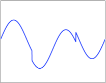
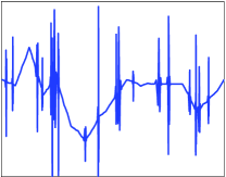
To illustrate the performance of the algorithm, we repeat the HeaviSine experiment from Figure 1. Recall that , and for this example. The advantages of using our tree-structured sparse approximation step (instead of mere hard thresholding) are evident from Figure 10. In practice, we have observed that our model-based algorithm converges in fewer steps than IHT and yields much more accurate results in terms of recovery error.
 |
 |
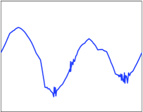 |
| (a) original | (b) IHT | (c) model-based IHT |
| (RMSE ) | (RMSE ) |
Appendix D Proof of Theorem 13
The proof of this theorem is identical to that of the CoSaMP algorithm in [11, Section 4.6], and requires a set of six lemmas. The sequence of Lemmas 1–6 below are modifications of the lemmas in [11] that are restricted to the structured sparsity model. Lemma 4 does not need any changes from [11], so we state it without proof. The proof of Lemmas 3–6 use the properties in Lemmas 1 and 2, which are simple to prove.
Lemma 1
Suppose has -RIP with constant . Let be a support corresponding to a subspace in . Then we have the following handy bounds.
Lemma 2
Suppose has -RIP with constant . Let be a support corresponding to a subspace in , and let . Then
We begin the proof of Theorem 13 by fixing an iteration of model-based CoSaMP. We write for the signal estimate at the beginning of the iteration. Define the signal residual , which implies that . We note that we can write .
Lemma 3
(Identification) The set , where , identifies a subspace in , and obeys
Proof of Lemma 3: Define the set . Let be the structured sparse approximation to with support , and similarly let be the approximation to with support . Each approximation is equal to for the coefficients in the support, and zero elsewhere. Since is the support of the best approximation in , we must have:
where denotes the set difference of and . These signals are in (since they arise as the difference of two elements from ); therefore, we can apply the -RIP constants and Lemmas 1 and 2 to provide the following bounds on both sides (see [11] for details):
| (22) | |||||
| (23) | |||||
Combining (22) and (23), we obtain
The argument is completed by noting that . ∎
Lemma 4
(Support Merger) Let be a set of at most indices. Then the set contains at most indices, and .
Lemma 5
(Estimation) Let be a support corresponding to a subspace in , and define the least squares signal estimate by , . Then
Proof of Lemma 5: It can be shown [11] that
Since is a support corresponding to a subspace in and , we use Lemmas 1 and 2 to obtain
Finally, note that . ∎
Lemma 6
(Pruning) The pruned approximation is such that
We use these lemmas in reverse sequence for the inequalities below:
From the recursion on , we obtain . This completes the proof of Theorem 13.∎
Appendix E Proof of Proposition 1
When , the number of subtrees of size of a binary tree of size is the Catalan number [49]
using Stirling’s approximation. When , we partition this count of subtrees into the numbers of subtrees of size and height , to obtain
We obtain the following asymptotic identity from [49, page 51]:
| (24) | |||||
We now simplify the formula slightly: we seek a bound for the sum term (which we denote by for brevity):
| (25) | |||||
Let , the value of for which the term inside the sum (25) is maximum; this is not necessarily an integer. Then,
where the second inequality comes from the fact that the series in the sum is strictly increasing for and strictly decreasing for . One of the terms in the sum can be added to one of the integrals. If we have that
| (26) |
then we can obtain
When the opposite of (26) is true, we have that
Since the term in the sum reaches its maximum for , we will have in all three cases that
We perform a change of variables and define to obtain
Using the formula for the fourth central moment of a Gaussian distribution:
we obtain
Thus, (24) simplifies to
Correspondingly, becomes
It is easy to show, using Euler-Maclaurin summations, that
we then obtain
This proves the proposition. ∎
Appendix F Proof of Proposition 3
We wish to find the value of the bound (12) for the subspace count given in (17). We obtain , where
We separate the terms that are linear on and , and obtain
The sequence is a decreasing sequence, since the denominators are decreasing sequences whenever . We then have
This completes the proof of Proposition 3. ∎
Acknowledgements
We thank Petros Boufounos, Mark Davenport, Yonina Eldar, Moshe Mishali, and Robert Nowak for helpful discussions.
References
- [1] S. Mallat, A Wavelet Tour of Signal Processing, Academic Press, San Diego, 1999.
- [2] D. L. Donoho, “Compressed sensing,” IEEE Trans. Info. Theory, vol. 52, no. 4, pp. 1289–1306, Sept. 2006.
- [3] E. J. Candès, “Compressive sampling,” in Proc. International Congress of Mathematicians, Madrid, Spain, 2006, vol. 3, pp. 1433–1452.
- [4] R. G. Baraniuk, “Compressive sensing,” IEEE Signal Processing Mag., vol. 24, no. 4, pp. 118–120, 124, July 2007.
- [5] V. Cevher, M. F. Duarte, C. Hegde, and R. G. Baraniuk, “Sparse signal recovery using Markov Random Fields,” in Proc. Workshop on Neural Info. Proc. Sys. (NIPS), Vancouver, Canada, Dec. 2008.
- [6] T. Blumensath and M. E. Davies, “Sampling theorems for signals from the union of finite-dimensional linear subspaces,” IEEE Trans. Info. Theory, vol. 55, no. 4, pp. 1872–1882, Apr. 2009.
- [7] Y. M. Lu and M. N. Do, “Sampling signals from a union of subspaces,” IEEE Signal Processing Mag., vol. 25, no. 2, pp. 41–47, Mar. 2008.
- [8] M. Stojnic, F. Parvaresh, and B. Hassibi, “On the reconstruction of block-sparse signals with an optimal number of measurements,” IEEE Trans. Signal Processing, vol. 57, no. 8, pp. 3075–3085, Aug. 2009.
- [9] Y. Eldar and M. Mishali, “Robust recovery of signals from a structured union of subspaces,” IEEE Trans. Info. Theory, vol. 55, no. 11, pp. 5302–5316, Nov. 2009.
- [10] D. Baron, M. F. Duarte, S. Sarvotham, M. B Wakin, and R. G. Baraniuk, “Distributed compressive sensing,” 2005, Preprint.
- [11] D. Needell and J. Tropp, “CoSaMP: Iterative signal recovery from incomplete and inaccurate samples,” Applied and Computational Harmonic Analysis, vol. 26, no. 3, pp. 301–321, May 2009.
- [12] M.A.T. Figueiredo and R.D. Nowak, “An EM algorithm for wavelet-based image restoration,” IEEE Trans. Image Processing, vol. 12, no. 8, pp. 906–916, 2003.
- [13] I. Daubechies, M. Defrise, and C. De Mol, “An iterative thresholding algorithm for linear inverse problems with a sparsity constraint,” Comm. Pure Appl. Math., vol. 57, pp. 1413–1457, 2004.
- [14] Emmanuel J. Candès and Justin K. Romberg, “Signal recovery from random projections,” in Proc. Computational Imaging III at SPIE Electronic Imaging, San Jose, CA, Jan. 2005, vol. 5674, pp. 76–86.
- [15] T. Blumensath and M. E. Davies, “Iterative threhsolding for sparse approximations,” Journal of Fourier Analysis and Applications, vol. 14, no. 5, pp. 629–654, Dec. 2008.
- [16] T. Blumensath and M. E. Davies, “Iterative hard thresholding for compressed sensing,” Applied and Computational Harmonic Analysis, vol. 27, no. 3, pp. 265–274, Nov. 2009.
- [17] M. S. Crouse, R. D. Nowak, and R. G. Baraniuk, “Wavelet-based statistical signal processing using hidden Markov models,” IEEE Trans. Signal Processing, vol. 46, no. 4, pp. 886–902, Apr. 1998.
- [18] R. G. Baraniuk, “Fast reconstruction from incoherent projections,” Workshop on Sparse Representations in Redundant Systems, May 2005.
- [19] M. F. Duarte, M. B. Wakin, and R. G. Baraniuk, “Fast reconstruction of piecewise smooth signals from random projections,” in Proc. SPARS05, Rennes, France, Nov. 2005.
- [20] C. La and M. N. Do, “Tree-based orthogonal matching pursuit algorithm for signal reconstruction,” in IEEE International Conference on Image Processing (ICIP), Atlanta, GA, Oct. 2006, pp. 1277–1280.
- [21] M. F. Duarte, M. B. Wakin, and R. G. Baraniuk, “Wavelet-domain compressive signal reconstruction using a hidden Markov tree model,” in IEEE Int. Conf. on Acoustics, Speech and Signal Processing (ICASSP), Las Vegas, NV, April 2008, pp. 5137–5140.
- [22] M. N. Do and C. N. H. La, “Tree-based majorize-minimize algorithm for compressed sensing with sparse-tree prior,” in International Workshop on Computational Advances in Multi-Sensor Adaptive Processing, Saint Thomas, US Virgin Islands, Dec. 2007, pp. 129–132.
- [23] L. He and L. Carin, “Exploiting structure in wavelet-based Bayesian compressive sensing,” IEEE Trans. Signal Processing, vol. 57, no. 9, pp. 3488–3497, Sep. 2009.
- [24] K. Lee and Y. Bresler, “Selecting good Fourier measurements for compressed sensing,” SIAM Conference on Imaging Science, July 2008.
- [25] S. Mendelson, A. Pajor, and N. Tomczak-Jaegermann, “Uniform uncertainty principle for Bernoulli and subgaussian ensembles,” Constructive Approximation, vol. 28, no. 3, pp. 277–289, Dec. 2008.
- [26] B. K. Natarajan, “Sparse approximate solutions to linear systems,” SIAM Journal on Computation, vol. 24, no. 2, pp. 227–234, Apr. 1995.
- [27] S. S. Chen, D. L. Donoho, and M. A. Saunders, “Atomic Decomposition by Basis Pursuit,” SIAM Journal on Scientific Computing, vol. 20, pp. 33, 1998.
- [28] J. Haupt and R. Nowak, “Signal reconstruction from noisy random projections,” IEEE Trans. Info. Theory, vol. 52, no. 9, pp. 4036–4048, Sept. 2006.
- [29] E. J. Candès and T. Tao, “The Dantzig selector: Statistical estimation when is much larger than ,” Annals of Statistics, vol. 35, no. 6, pp. 2313–2351, Dec. 2007.
- [30] J. Tropp and A. C. Gilbert, “Signal recovery from partial information via orthogonal matching pursuit,” IEEE Trans. Info. Theory, vol. 53, no. 12, pp. 4655–4666, Dec. 2007.
- [31] D. L. Donoho, I. Drori, Y. Tsaig, and J. L. Starck, “Sparse solution of underdetermined linear equations by stagewise orthogonal matching pursuit,” 2006, Preprint.
- [32] W. Dai and O. Milenkovic, “Subspace pursuit for compressive sensing: Closing the gap between performance and complexity,” IEEE Trans. Info. Theory, vol. 55, no. 5, pp. 2230–2249, May 2009.
- [33] E. J. Candès, “The restricted isometry property and its implications for compressed sensing,” Compte Rendus de l’Academie des Sciences, Series I, vol. 346, no. 9–10, pp. 589–592, May 2008.
- [34] R. G. Baraniuk and D. L. Jones, “A signal-dependent time-frequency representation: Fast algorithm for optimal kernel design,” IEEE Trans. Signal Processing, vol. 42, no. 1, pp. 134–146, Jan. 1994.
- [35] R. G. Baraniuk, “Optimal tree approximation with wavelets,” in Wavelet Applications in Signal and Image Processing VII, Denver, CO, July 1999, vol. 3813 of Proc. SPIE, pp. 196–207.
- [36] R. G. Baraniuk, R. A. DeVore, G. Kyriazis, and X. M. Yu, “Near best tree approximation,” Advances in Computational Mathematics, vol. 16, no. 4, pp. 357–373, May 2002.
- [37] J. K. Romberg, H. Choi, and R. G. Baraniuk, “Bayesian tree-structured image modeling using wavelet-domain hidden Markov models,” IEEE Trans. Image Processing, vol. 10, no. 7, pp. 1056–1068, July 2001.
- [38] J. Portilla, V. Strela, M. J. Wainwright, and E. P. Simoncelli, “Image denoising using a scale mixture of Gaussians in the wavelet domain,” IEEE Trans. Image Processing, vol. 12, no. 11, pp. 1338–1351, Nov. 2003.
- [39] J. Shapiro, “Embedded image coding using zerotrees of wavelet coefficients,” IEEE Trans. Signal Processing, vol. 41, no. 12, pp. 3445–3462, Dec. 1993.
- [40] A. Cohen, W. Dahmen, I. Daubechies, and R. A. DeVore, “Tree approximation and optimal encoding,” Applied and Computational Harmonic Analysis, vol. 11, no. 2, pp. 192–226, Sept. 2001.
- [41] D. Donoho, “CART and best ortho-basis: A connection,” Annals of Statistics, vol. 25, no. 5, pp. 1870–1911, Oct. 1997.
- [42] M. B. Wakin, S. Sarvotham, M. F. Duarte, D. Baron, and R. G. Baraniuk, “Recovery of jointly sparse signals from few random projections,” in Proc. Workshop on Neural Info. Proc. Sys. (NIPS), Vancouver, Nov. 2005.
- [43] J. Tropp, A. C. Gilbert, and M. J. Strauss, “Algorithms for simultaneous sparse approximation. Part I: Greedy pursuit,” Signal Processing, vol. 86, no. 3, pp. 572–588, Apr. 2006.
- [44] M. F. Duarte, V. Cevher, and R. G. Baraniuk, “Model-based compressive Sensing for Signal Ensembles,” in Allerton Conference on Communication, Control, and Computing, Monticello, IL, Oct. 2009.
- [45] C. Hegde, M. F. Duarte, and V. Cevher, “Compressive sensing recovery of spike trains using a structured sparsity model,” in Workshop on Signal Processing with Adaptive Sparse Structured Representations (SPARS), Saint Malo, France, Apr. 2009.
- [46] V. Cevher, P. Indyk, C. Hegde, and R. G. Baraniuk, “Recovery of clustered sparse signals from compressive measurements,” in Int. Conf. on Sampling Theory and Applications (SAMPTA), Marseille, France, May 2009.
- [47] E. J. Candès and T. Tao, “Decoding by linear programming,” IEEE Trans. Info. Theory, vol. 51, pp. 4203–4215, Dec. 2005.
- [48] M. Ledoux, The Concentration of Measure Phenomenon, American Mathematical Society, 2001.
- [49] G. G. Brown and B. O. Shubert, “On random binary trees,” Mathematics of Operations Research, vol. 9, no. 1, pp. 43–65, Feb. 1984.