A sphere moving down the surface of a static sphere and a simple phase diagram.

Abstract

A small sphere placed on the top of a big static frictionless sphere, slips until it leaves the surface at an angle $\theta_{l}=\cos^{-1}{2/3}$. On the other extreme, if the surface of the big sphere has coefficient of static friction, $\mu_{s}\rightarrow\infty$, the small sphere starts rolling and continues to do so until it leaves the surface at an angle $\theta_{l}=\cos^{-1}{10/17}$. In the case where, $0<\mu_{s}<\infty$, we get a simple phase diagram. The three phases are pure rolling, rolling with slipping and detached state. One phase line separates pure rolling from rolling with slipping. This diagram is obtained when stopping angles for pure rolling are plotted against static friction coefficients $\mu_{s}$. Study in this article is restricted to the case when the mobile sphere starts at the top of the static sphere with infinitesimal kinetic energy.

I Introduction

An interesting text book problem in the introductory mechanics([1], [2], [3]) is to determine the release point for a block of mass m. The block slides without friction on the surface of a static sphere of radius R. The block starts from ”rest”, i.e. with infinitesimal velocity, from the top of the sphere. The block looses contact with the sphere, by the time it travels a vertical distance $\frac{R}{3}$. This is equivalent to an angular displacement $cos^{-1}\frac{2}{3}$. This result draws attention. The angular displacement does not depend either on the mass of the block or, the radius of the sphere. The result is general.
When there is friction on the surface of a sphere ([4], [5], [6]), the block leaving with infinitesimal velocity at the top of the static sphere, immediately stops. This dull situation changes to better as soon as the block is given a finite velocity at the top of the static sphere. The block may now continue to slip. It may also get released from the surface of the sphere below. Whether the block will leave the sphere below or, stick depends on the amount of friction. In that sense, the initial velocity and the static friction start playing with the block in fixing the fate of it. In an interesting report ([6]), the authors got an exact relation between initial velocity and the coefficient of static friction, requiring the block to be released from the surface with zero velocity. Once drawn by them([6]), two features appeared. The plot resembles $tanh$ curve. The curve separates two regions on the plot clearly. The lower region refers to the set of possibilities when the block will stick. The upper region tells us when the block will leave.
Once the block is replaced by a sphere, two things occur. In the case the coefficient of static friction is zero([7]), the mobile sphere slides and leaves the surface exactly as the block does. When the coefficient of static friction is very large([7]) and tends to infinity, the mobile sphere instead of stopping immediately as in the case of the block, starts doing something else. It starts to pure roll. It pure rolls until it leaves the surface. As the coefficient of static friction is retained intermediate between these two extreme limits, zero and infinity, feasibility of a new kind of motion arises. The sphere pure rolls initially, then starts skidding along with rolling ([8], [9]). This going over to mixed rolling happens at a particular angle. The mobile sphere, once trapped in the mixed rolling phase, continues to do so until it leaves the surface of the static sphere.
Incidentally, the cross-over angle bears a simple relationship with the coefficient of static friction. This refers to cross-over from pure to mixed rolling. Once the cross-over angle is plotted, against the coefficient of static friction, two features appear. The plot bears resemblance with $tanh$ curve. The curve separates two regions on the plot clearly. The lower region refers to the set of possibilities when the mobile object sticks to the pure rolling phase. The upper region refers to the mixed rolling phase. These qualitative features of the phase diagram seem to be general, independent of the nature of the movable object, whether it is a block, or, a sphere.
The phase diagram in the case of Mele et.al. ([6]), is external. Both the axes, initial velocity and coefficient of static friction, refer to parameters controlled from outside. In the case of a mobile sphere, the phase plot is apparently partly internal. The parameter $\theta$ though may appear internal, refers to the scale for potential energy, which is tuned from below, just as the coefficient of static friction is. If $v$ in the case of Mele et.al. ([6]), determines the initial kinetic energy given to the block, varying $\theta$ in the case of riding sphere, implies going over from one potential energy to another. Though we have only one initial kinetic energy for a set-up, we have an infinite sequence of potential energies for the same set-up, the sequence marked by $\theta$.As the initial velocity of the movable sphere, at the top, is changed from zero to non-zero, a mixed rolling phase is likely to appear in the resulting three dimensional, ($v$, $\theta$, $\mu_{s}$), phase diagram.
In the section II, the motion of the small sphere at the top of a static sphere is dealt with in the context of the frictionless case. In the following section III, the angle at which the mobile sphere leaves the static sphere, in the case of infinite friction, is derived. In the section IV, the intermediate coefficient of static friction is considered, with the depiction of consequent phase diagram. In the subsection IV.1, the general expression for the release angle is arrived at, followed by a diagram of $\theta_{l}$ against $\theta_{0}$. In the next subsection, we determine the order parameter and a critical exponent associated with the phase transition at $\theta_{0}$.

II $\mu_{s}=0$

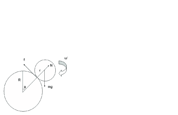
Figure 1: The small sphere is rolling down the big static sphere

As the Fig.1 illustrates, three forces are acting on the small sphere. The normal force, $N$, is acting through the contact surface, along the line joining the centers. The weight of the small sphere, $mg$, is passing through the center of mass vertically downwards. The static frictional force is being exerted by the static sphere below, through the surface of contact, opposite to the direction of motion. The motion of the center of mass of the small sphere, until it leaves the surface of the big sphere is a circle about the center of the big sphere. This makes, use of planar polar coordinate system for the description of motion particularly handy, with the the center of the big sphere as the origin and the top most position chosen as $\theta=0$. Velocity of the center of mass, $v$, then reduces to $(R+r)\omega$. Acceleration of the center of mass of the small sphere, splits up into radial acceleration $\frac{v^{2}}{r+R}$ and cross-radial acceleration $(R+r)\frac{d\omega}{dt}$. Newton’s second law yields radial and cross-radial equations of motion. The radial equation of motion is,

$$mgcos(\theta)-N(\theta)=\frac{mv^{2}}{r+R}$$ (1)

In this case, as friction is absent, integration of cross-radial equation of motion with respect to $\theta$, leads to the energy conservation equation,

$$\frac{1}{2}mv^{2}-mg(r+R)(1-cos\theta)=0$$ (2)

As the small sphere leaves the surface of the big sphere,

$$N(\theta)=0.$$ (3)

This fact together with the equations (1) and (2), yields a quantitative expression for the release angle,

$$\theta=\cos^{-1}{2/3}=0.8411.$$ (4)

III $\mu_{s}\rightarrow\infty$

The small sphere, given a small perturbation, starts rolling without slipping. The radial equation remains as before for the $\mu_{s}=0$ case. The energy conservation equation(2) modifies to

$$\frac{1}{2}mv^{2}+\frac{1}{2}I(\omega^{\prime})^{2}-mg(r+R)(1-cos\theta)=0.$$ (5)

where, $\omega^{\prime}$ refers to angular velocity with respect to the center of mass of the small sphere. $I$ in the above equation(5) corresponds to the moment of inertia for the small sphere,

$$I=\frac{2}{5}mr^{2}.$$ (6)

During pure rolling,

$$v=\omega^{\prime}r.$$ (7)

This fact combined with the radial and energy conservation equations, (1,5) added with the equation (3) yields the angle of release

$$\theta=\cos^{-1}{10/17}=0.9419.$$ (8)

$\mu_{s}\rightarrow\infty$ guaranties that the small sphere continues to pure roll without going over to slipping, until it takes off from the surface of the sphere below.

IV $0<\mu_{s}<\infty$

The cross radial equation of motion in this case appears as,

$$ma_{\theta}=F_{\theta},$$ (9)

with,

$$F_{\theta}=mgsin\theta-f,$$ (10)

being the cross radial force. The torque equation for rotation of the small sphere about its center of mass, is

$$I\alpha^{\prime}=rf$$ (11)

where, $f$, is the static frictional force acting on the small sphere. This is acting tangentially at the point of contact with the sphere below. Since, the velocity of the center of mass of the small sphere is in the cross-radial direction, the equation (7) for pure rolling can be written as,

$$a_{\theta}=r\alpha^{\prime}$$ (12)

These three equations (9), (11), (12), once combined, lead to a simple dependence of angular position, $\theta$, on the frictional force, for the pure rolling to persist,

$$f=\frac{2}{7}mgsin\theta.$$ (13)

Related matters are dealt with in a slightly different context in the references ([8], [9]). As $\theta$ increases, $f$ increases. At one angle, ([10]), $f$ reaches its maximum value

$$f_{max}=\mu_{s}N.$$ (14)

Beyond that angle, denoted as $\theta_{0}$, the pure rolling demands value of $f$ more than $\mu_{s}N$. As this is not possible, the small sphere starts to slip and roll simultaneously. In other words, at that angle $\theta_{0}$, pure rolling stops. This feature has been discussed well, in the context of motion of a cylinder on a cylinder, in a beautiful paper of Flores et.al.([11]). Along with it, as long as the small sphere pure rolls, there is no loss of energy. The energy conservation equation (5) remains the same,

$$\frac{1}{2}mv^{2}+\frac{1}{2}I(w^{\prime})^{2}-mg(r+R)(1-cos\theta)=0$$ (15)

This equation, in this case of pure rolling, is equivalent to

$$\frac{v^{2}}{r+R}=\frac{10}{7}g(1-cos\theta).$$ (16)

In the eq.(13) at the angle, $\theta_{0}$, at which the small sphere starts to slip, takes the form,

$$\mu_{s}N(\theta_{0})=\frac{2}{7}mgsin\theta_{0}$$ (17)

Consequently, the radial equation of motion (1)

$$N(\theta_{0})=mgcos\theta_{0}-\frac{mv^{2}}{R+r}$$ (18)

together with the energy conservation equation (16), leads to an implicit equation for $\theta_{0}$,

$$\mu_{s}=\frac{2sin\theta_{0}}{17cos\theta_{0}-10}$$ (19)

The plot against the static friction coefficient $\mu_{s}$, of the angle, $\theta_{0}$, at which the small sphere starts slipping along with rolling, is shown in the Fig.2. Interesting part of it is that, the eq.(19) does not depend on any of the radii of the two spheres involved.

Figure 2: Plot of stopping angles for pure rolling against static friction coefficients

The upper part of the phase diagram, in principle, can split into two parts. One in which the mobile sphere remains on the static sphere while doing mixed rolling. Another in which the mobile sphere has left the surface of the static sphere. This second line, obviously, will start from $\theta=cos^{-1}\frac{2}{3}$ and will meet the first line (eq.19), at $\mu_{s}\rightarrow\infty$

IV.1 Determination of angle of release, $\theta_{l}$

Once the mobile sphere starts skidding, kinetic friction comes into play. The frictional force is given by, ([10]),

$$f_{k}=\mu_{k}N$$ (20)

where, $\mu_{k}$ is constant. The cross radial equation of motion, (9), takes the form

$$ma_{\theta}=mgsin\theta-\mu_{k}N.$$ (21)

This equation, eq.(21), combined with the radial equation, eq.(1), leads to a first order differential equation for $\omega$,

$$\frac{d\omega}{dt}-\mu_{k}\omega^{2}=\frac{g}{r+R}(sin\theta-\mu_{k}cos\theta).$$ (22)

Integration, a.la Mele et.al.([4]) of the above equation, results in an expression for $\omega$ for an angle greater than the cross-over angle, $\theta_{0}$,
$\omega^{2}(\theta)=\omega^{2}(\theta_{0})e^{2\mu_{k}(\theta-\theta_{0})}-\frac{2g}{(r+R)(1+4\mu_{k}^{2})}[cos\theta(1-2\mu_{k}^{2})\\ +3\mu_{k}sin\theta-(cos\theta_{0}(1-2\mu_{k}^{2})+3\mu_{k}sin\theta_{0})e^{2\mu_{k}(\theta-\theta_{0})}]$

This expression when supplemented with the equations, (3), (1), (16), leads to an illuminating relation,
$3cos\theta_{l}+6\mu_{k}sin\theta_{l}=e^{2\mu_{k}(\theta_{l}-\theta_{0})}[6\mu_{k}sin\theta_{0}+\frac{4-68\mu_{k}^{2}}{7}\\ cos\theta_{0}+\frac{10}{7}(1+4\mu_{k}^{2})].$ Once complemented with the equation, (19), this is an expression for $\theta_{l}$ in terms of $\mu_{s}$ and $\mu_{k}$. One interesting simplification occurs for $\mu_{k}=\mu_{s}$. Then as described just before this subsection, it becomes crystal clear, see the Fig.3, that the three phase lines separating pure rolling, mixed rolling, detached phases, meet at one point. The point is $\theta_{l}=cos^{-1}\frac{10}{17}=\theta_{0}$. This is reminiscent of the triple point in the solid-liquid-gas phase transitions.

Figure 3: Plot of release angles against cross-over angles

IV.2 Order parameter

As long as the sphere pure rolls, $\frac{v}{\omega r}$ is one. As it starts mixed rolling, $\frac{v}{\omega r}$ starts increasing from one continuously. Hence, $2\pi(\frac{v}{\omega r}-1)$ acts like an order parameter, $\eta$, of second order phase transition [12, 13, 14]. Here the phase transition is intrinsically a non-equilibrium [15, 16] one. Physically, the introduced order parameter refers to the deficit angle a point on the sphere is lagging by in terms of rotation per second, in comparison to a hypothetical pure rolling sphere. Analogues of $\Omega$ and $\Omega_{c}$ in Fig.3b. of ref.([13]) are the static frictions given by the equations, (13) and (14). We observe,

$$\eta=\pi\mu_{k}(5+\frac{2-\frac{5\mu_{s}}{\mu_{k}}+cos\theta_{0}(\frac{17}{2}\frac{\mu_{s}}{\mu_{k}}-\frac{11}{2})}{1-cos\theta_{0}})\frac{sin\theta_{0}}{cos\theta_{0}}(1-\frac{f_{max}}{f})$$ (23)

Hence, we get a critical exponent $1$.

V Acknowledgement

The authors would like to thank Anupam and Saiteja for help with plotting.

VI Suggested Problems

The three dimensional, ($\theta_{l},\mu_{s},\mu_{k}$), phase diagram can be easily drawn using Mathematica7. The phase diagram for the case when the small sphere starts with an initial kinetic energy, has been done for $\frac{v_{0}}{\omega_{0}r}=1$ in ref. [17]. Moreover, it will be interesting to have a full qualitative analysis of motion of a sphere on a static sphere following Flores et.al.([11]). Exploring the consequences of replacing the static sphere by, say, a static cycloidal hill ([7]), along the line of this article, is as much desirable.

References

- [1] D. Halliday, R. Resnick, and J.A. Walker, Fundamentals of Physics (Wiley, New York, 2005). 7th extended ed., Chap. 8, Prob. 36.
- [2] D. Kleppner and R. J. Kolenkow, An Introduction to Mechanics (McGraw-Hill, Boston, 1973), Prob. 4.6.
- [3] Gerald E. Hite, ” The sled race”, Am. J. Phys. 72(8), 1055-58(2004).
- [4] Tom Prior and E. J. Mele, ” A block slipping on a sphere with friction: Exact and Perturbative solutions” Am. J.Phys. 75,423-426(2007).
- [5] C. E. Mungan, ” Sliding on the surface of a rough sphere”, Phys. Teach. 41, 326-328(2003).
- [6] O. L. de Lange, J. Pierrus, Tom Prior and E. J. Mele, Am. J. Phys. 76(1), 92-93(2008).
- [7] M. R. Spiegel, Theoretical Mechanics (Schaum’s outline series, McGraw-Hill, Singapore, 1982), Problems 3.23, 9.42, 9.143 (pp. 76, 244, 252).
- [8] R. A. Bachman, ” Sphere rolling down a grooved track”, Am. J. Phys. 53(8), 765-767(1985).
- [9] Qing-gong Song, ” The requirement of a sphere rolling without slipping down a grooved track for the coefficient of static friction”, Am. J. Phys. 56(12), 1145-1146(1988).
- [10] A. Sommerfield, Mechanics (Levant Books, Kolkata, 2003) pp. 81-83.
- [11] J. Flores et.al., ” A simple problem in mechanics: A qualitative approach”, Am. J. Phys. 40, 595-598(1972).
- [12] R. Alben, ” An exactly solvable model exhibiting a Landau phase transition”, Am. J. Phys. 40, 3(1972).
- [13] Jean Sivardiere, ” A simple mechanical model exhibiting a spontaneous symmetry breaking”, Am. J. Phys. 51, 1016(1983).
- [14] G. Fletcher, ” A mechanical analog of first- and second-order phase transitions”, Am. J. Phys. 65, 74(1997).
- [15] M. Einax, M. Schulz, S. Trimper, ” Friction and second-order phase transition”, Phys Rev E 70, 046113(2004).
- [16] M. Peyrard, S. Aubry, ” Critical behaviour at the transition by breaking of analyticity in the discrete Frenkel-Kontorova model”.
- [17] ’”Studying Phase transitions in Mechanical models using MATLAB/ Mathematica” - Report by Puneet Chaganti, 2005A3PS207G, submitted in partial fulfillment of the course BITS GC335’