Conditional probability based significance tests for sequential patterns in multi-neuronal spike trains

Abstract

In this paper we consider the problem of detecting statistically significant sequential patterns in multi-neuronal spike trains. These patterns are characterized by an ordered sequences of spikes from different neurons with specific delays between spikes. We have previously proposed a datamining scheme [21] to efficiently discover such patterns which are frequent in the sense that the count of non-overlapping occurrences of the pattern in the data stream is above a threshold. Here we propose a method to determine the statistical significance of these repeating patterns and to set the thresholds automatically. The novelty of our approach is that we use a compound null hypothesis that includes not only models of independent neurons but also models where neurons have weak dependencies. The strength of interaction among the neurons is represented in terms of certain pair-wise conditional probabilities. We specify our null hypothesis by putting an upper bound on all such conditional probabilities. We construct a probabilistic model that captures the counting process and use this to calculate the mean and variance of the count for any pattern. Using this we derive a test of significance for rejecting such a null hypothesis. This also allows us to rank-order different significant patterns. We illustrate the effectiveness of our approach using spike trains generated from a non-homogeneous Poisson model with embedded dependencies.

1 Introduction

Analyzing spike trains from hundreds of neurons to find significant temporal patterns is an important current research problem [7, 25, 22]. By using experimental techniques such as Micro Electrode Arrays or imaging of neural currents, spike data can be recorded simultaneously from many neurons [12, 30]. Such multi-neuronal spike train data can now be routinely gathered in vitro from neural cultures or in vivo from brain slices, awake behaving animals and even humans. Such data would be a mixture of stochastic spiking activities of individual neurons as well as that due to correlated activity of groups of neurons due to interconnections, possibly triggered by external inputs. Automatically discovering patterns (regularities) in these spike trains can lead to better understanding of how interconnected neurons act in a coordinated manner to generate specific functions. There has been much interest in techniques for analyzing the spike data so as to infer functional connectivity or the functional relationships within the system that produced the spikes [3, 6, 27, 11, 7, 14, 9, 24, 12, 19, 25, 22, 10]. In addition to contributing towards our knowledge of brain function, understanding of functional relations embedded in spike trains leads to many applications, e.g., better brain-machine interfaces. Such an analysis can also ultimately allow us to systematically address the question, "is there a neural code?".

In this paper, we consider the problem of discovering statistically significant patterns from multi-neuronal spike train data. The patterns we consider here are ordered firing sequences by a group of neurons with specific time-lags or delays between successive neurons. Such a pattern (when it repeats many times) may denote a chain of triggering events and hence unearthing such patterns from spike data can help understand the underlying functional connectivity. For example, memory traces are probably embedded in such sequential activation of neurons and signals of this form have been found in hippocampal neurons [18]. Such patterns of ordered firing sequences with fairly constant delays between successive neuronal firings have been observed in many experiments and there is much interest in detecting such patterns and assessing their statistical significance. (See [2, 11] and references therein).

Here, we will call patterns of ordered firing sequences as sequential patterns. Symbolically, we denote such a pattern as, e.g., $A\stackrel{{\scriptstyle T_{1}}}{{\rightarrow}}B\stackrel{{\scriptstyle T_{2}}}{{\rightarrow}}C$. This represents the pattern of ordered firing sequence of $A$ followed by $B$ followed by $C$ with a delay of $T_{1}$ time units between $A$ & $B$ and $T_{2}$ time units between $B$ & $C$. (We note here that within any occurrence of such a firing pattern, there could be spikes by other neurons). Such a pattern of firings may occur repeatedly in the spike train data if, e.g., there is an excitatory influence of total delay $T_{1}$ from $A$ to $B$ and an excitatory influence of delay $T_{2}$ between $B$ and $C$. In general, the delays may not be exactly constant because synaptic transmission etc. could have some random variations. Hence, in our sequential patterns, we will allow the delays to be intervals of small length. At the least, we can take the length of the interval as the time resolution in our measurements. In general, such patterns can involve more than three neurons. The size of a pattern is the number of neurons in it. Thus, the above example is that of a size 3 pattern or a 3-node pattern.

One of the main computational methods for detecting such patterns that repeat often enough, is due to Abeles and Gerstein [3]. This essentially consists of sliding the spike train of one neuron with respect to another and noting coincidences at specific delays. There are also some recent variations of this method [26, 28]. Most of the current methods for detecting such patterns essentially use correlations among time-shifted spike trains (and some statistics computed from the correlation counts), and these are computationally expensive when detecting large-size (typically greater than 4) patterns [11]. Another approach to detecting such ordered firing sequences is considered in [19, 25] while analyzing recordings from hippocampal neurons. Given a specific ordering on a set of neurons, they look for longest sequences in the data that respect this order. This is similar to our sequential patterns which are somewhat more general because we can also specify different delays between consecutive elements of the pattern.

In this paper we use a method based on some temporal datamining techniques that we have recently proposed [21]. This method can automatically detect all sequential patterns whose frequency in the data is above a (user-specified) threshold where frequency of the pattern is maximum number of non-overlapped occurrences of the pattern in the spike data. The essence of this algorithm is that instead of trying to count all occurrences of the pattern in the data we count only certain well-defined subset of occurrences and this makes the process computationally efficient. The method is effective in detecting long patterns and it would detect only those patterns that repeat more than a given threshold. Also, the method can automatically decide on the most appropriate delays in each detected pattern by choosing from a set of possible delays supplied by the user. (See [21] for details).

The main contribution of this paper is a method for assessing the statistical significance of such sequential patterns. The objective is to have a method so that we will detect only those patterns that repeat often enough to be significant (and thus fix the thresholds for the data mining algorithm automatically). We tackle this issue in a classical hypothesis testing framework.

There have been many approaches for assessing the significance of detected firing patterns [2, 11, 19, 25, 10]. In the current analytical approaches, one generally employs a Null hypothesis that the different spike trains are generated by independent processes. In most cases one assumes (possibly inhomogeneous) Bernoulli or Poisson processes. Then one can calculate the probability of observing the given number of repetitions of the pattern (or of any other statistic derived from such counts) under the null hypothesis of independent processes and hence calculate a minimum number of repetitions needed to conclude that a pattern is significant in the sense of being able to reject the null hypothesis. There are also some empirical approaches suggested for assessing significance [8, 2, 11, 31]. Here one creates many surrogate data streams from the experimentally observed data by perturbing the individual spikes while keeping certain statistics same and then assessing significance by noting whether or not the patterns are preserved in the surrogate data. There are many possibilities for the perturbations to be imposed to generate surrogate data [11]. In these empirical methods also, the implicit null hypothesis assumes independence.

The main motivation for the approach presented here is the following. If a sequential pattern repeats often enough to be significant then one would like to think that there are strong influences among the neurons representing the pattern. However, different (detected) patterns may represent different levels or strengths of influences among their constituent neurons. Hence it would be nice to have a method of significance analysis that can rank order different (significant) patterns in terms some ‘strength of influence’ among the neurons of the pattern. For this, here we propose that the strength of influence of $A$ on $B$ is well represented by the conditional probability that $B$ will fire after some prescribed delay given that $A$ has fired. We then employ a composite null hypothesis specified through one parameter that denotes an upper bound on all such pairwise conditional probabilities. Using this we would be able to decide whether or not a given pattern is significant at various values for this parameter in the null hypothesis and thus be able to rank-order different patterns.

There is an additional and important advantage of the above approach that we propose here. Our composite null hypothesis is such that any stochastic model for a set of spiking neurons would be in the null hypothesis if all the relevant pairwise conditional probabilities are below some bound. Since this bound is a parameter that can be chosen by the user, the null hypothesis would include not only independent neuron models but also many models of interdependent neurons where the pair-wise influences among neurons are ‘weak’. Hence rejecting such a null hypothesis is more attractive than rejecting a null hypothesis of independence when we want to conclude that a significant pattern indicates ‘strong’ interactions among the neurons. In this sense, the approach presented here extends the currently available methods for significance analysis.

We analytically derive some bounds on the probability that our counting process would come up with a given number of repetitions of the firing pattern if the data is generated by any model that is contained in our compound null hypothesis. As mentioned earlier, we use the number of non-overlapped occurrences of a pattern as our test statistic instead of the total number of repetitions and employ a temporal datamining algorithm for counting non-overlapped occurrences of sequential patterns [21]. This makes our method attractive for discovering significant patterns involving large number of neurons also. We show the effectiveness of the method through extensive simulation experiments on synthetic spike train data obtained through a model of inter-dependent non-homogeneous Poisson processes.

The rest of the paper is organized as follows. In section 2 we give a brief overview of temporal datamining and explain our algorithm for detecting sequential patterns whose frequency is above some threshold. The full details of the algorithm are available elsewhere [21, 29] and we provide only some details which are relevant for understanding the statistical significance analysis which is presented in section 3. In section 4, we present some simulation results on synthetic spike train data to show the effectiveness of our method. We present results to show that our method is capable of ranking different patterns in terms of the synaptic efficacy of the connections. While we confine our attention in this paper to only sequential patterns, the statistical method we present can be generalized to handle other types of patterns. We briefly indicate this and conclude the paper with a discussion in section 5.

2 Frequent Episodes Framework for discovery of sequential patterns

Temporal datamining is concerned with analyzing symbolic time series data to discover ‘interesting’ patterns of temporal dependencies [15, 20]. Recently we have proposed that some datamining techniques, based on the so called frequent episodes framework, are well suited for analyzing multi-neuronal spike train data [21]. Many patterns of interest in spike data such as synchronous firings by groups of neurons, the sequential patterns explained in the previous section, and synfire chains which are a combination of synchrony and ordered firings, can be efficiently discovered from the data using these datamining techniques. While the algorithms are seen to be effective through simulations presented in [21], no statistical theory was presented there to address the question of whether the detected patterns are significant in any formal sense which is the main issue addressed in this paper. In this section we first briefly outline the frequent episodes framework and then qualitatively describe this datamining technique for discovering frequently occurring sequential patterns.

In the frequent episodes framework of temporal datamining. the data to be analyzed is a sequence of events denoted by $\langle(E_{1},t_{1}),(E_{2},t_{2}),\ldots\rangle$ where $E_{i}$ represents an event type and $t_{i}$ the time of occurrence of the $i^{th}$ event. $E_{i}$’s are drawn from a finite set of event types, $\zeta$. The sequence is ordered with respect to time of occurrences of the events so that, $t_{i}\leq t_{i+1}$, $\forall i$. The following is an example event sequence containing 11 events with 5 event types.

$$\langle(A,1),(B,3),(D,5),(A,5),(C,6),(A,10),(E,15),(B,15),(B,17),(C,18),(C,19)\rangle$$ (1)

In multi-neuronal spike data, the event type of a spike event is the label of the neuron which generated the spike and the event has the associated time of occurrence. The neurons in the ensemble under observation fire action potentials at different times, that is, generate spike events. All these spike events are strung together, in time order, to give a single long data sequence as needed for frequent episode discovery. It may be noted that there can be more than one event with the same time because two neurons can spike at the same time.

The temporal patterns that we wish to discover in this framework are called episodes. In general, episodes are partially ordered sets of event types. Here we are only interested in serial episodes which are totally ordered.

A serial episode is an ordered tuple of event types. For example, $(A\rightarrow B\rightarrow C)$ is a 3-node serial episode. (We also say that the size of this episode is 3). The arrows in this notation indicate the order of the events. Such an episode is said to occur in an event sequence if there are corresponding events in the prescribed order in the data sequence. In sequence (1), the events {${(A,1),(B,3),(C,6)}$} constitute an occurrence of the serial episode $(A\rightarrow B\rightarrow C)$ while the events {$(B,3),(C,6),(A,10)$} do not. We note here that occurrence of an episode does not require the associated event types to occur consecutively; there can be other intervening events between them.

In the multi-neuronal data, if neuron $A$ makes neuron $B$ to fire, then, we expect to see $B$ following $A$ often. However, in different occurrences of such a substring, there may be different number of other spikes between $A$ and $B$ because many other neurons may also be spiking during this time. Thus, the episode structure allows us to unearth patterns in the presence of such noise in spike data.

The objective in frequent episode discovery is to detect all frequent episodes (of different lengths) from the data. A frequent episode is one whose frequency exceeds a (user specified) frequency threshold. The frequency of an episode can be defined in many ways. It is intended to capture some measure of how often an episode occurs in an event sequence. One chooses a measure of frequency so that frequent episode discovery is computationally efficient and, at the same time, higher frequency would imply that an episode is occurring often.

Here, we define frequency of an episode as the maximum number of non-overlapped occurrences of the episode in the data stream. Two occurrences of an episode are said to be non-overlapped if no event associated with one occurrence appears in between the events associated with the other. A set of occurrences is said to be non-overlapped if every pair of occurrences in it are non-overlapped. In our example sequence (1), there are two non-overlapped occurrences of $A\rightarrow B\rightarrow C$ given by the events: $((A,1),(B,3),(C,6))$ and $((A,10),(B,15),(C,18))$. Note that there are three distinct occurrences of this episode in the data sequence though we can have only a maximum of two non-overlapped occurrences. We also note that if we take the occurrence of the episode given by $((A,1),(B,15),(C,18))$, then there is no other occurrence that is non-overlapped with this occurrence. That is why we define the frequency to be the maximum number of non-overlapped occurrences.

This definition of frequency results in very efficient counting algorithms with some interesting theoretical properties [16, 17]. In addition, in the context of our application, counting non-overlapped occurrences seems natural because we would then be looking at chains that happen at different times again and again.

In analyzing neuronal spike data, it is useful to consider methods, where, while counting the frequency, we include only those occurrences which satisfy some additional temporal constraints. Here we are interested in what we call inter-event time constraint which is specified by giving an interval of the form $(T_{low},T_{high}]$. The constraint requires that the difference between the times of every pair of successive events in any occurrence of a serial episode should be in this interval. In general, we may have different time intervals for different pairs of events in each serial episode. As is easy to see, a serial episode with inter-event time constraints corresponds to what we called a sequential pattern in the previous section. These are the temporal patterns of interest in this paper.

The inter-event time constraint allows us to take care of delays involved in the process of one neuron influencing another through a synapse. Suppose neuron $A$ is connected to neuron $B$ which, in turn, is connected to neuron $C$, through excitatory connections with delays $T_{1}$ and $T_{2}$ respectively. Then, we should be counting only those occurrences of the episode $A\rightarrow B\rightarrow C$, where the inter-event times satisfy the delay constraint. This would be the sequential pattern $A\stackrel{{\scriptstyle T_{1}}}{{\rightarrow}}B\stackrel{{\scriptstyle T_{2}}}{{\rightarrow}}C$. In general, the inter-event constraint could be an interval. Occurrences of such serial episodes with inter-event constraints in spike data are shown schematically in fig. 1

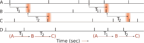
Figure 1: A schematic showing two occurrences of the sequential pattern $A\stackrel{{\scriptstyle T_{1}}}{{\rightarrow}}B\stackrel{{\scriptstyle T_{2}}}{{\rightarrow}}C$ in the spike trains from neurons $A,B,C,D$. A small interval (usually 1 ms) is shown around the second and third spike to indicate possible variation in the delay. Note that within the duration of one occurrence of the pattern there may be other intervening spikes (from any of the neurons).

In any occurrence of the episode or sequential pattern, we call the difference between the times of the first and last events as its span. The span would be the total of all the delays. If, in the above episode, the span of all occurrences would be $T_{1}+T_{2}$ and hence we may call it the span of the episode. If the inter-event time constraints are intervals then the span of different occurrences could be different.

There are efficient algorithms for discovering all frequent serial episodes with specified inter-event constraints [21]. That is, for discovering all episodes whose frequency (which is the number of non-overlapped occurrences of the episode) is above a given threshold.

Conceptually, the algorithm does the following. Suppose, we are operating at a time resolution of $\Delta T$. (That is, the times of of events or spikes are recorded to a resolution of $\Delta T$). Then we discretize the time axis into intervals of length $\Delta T$. Then, for each episode whose frequency we want to find we do the following. Suppose the episode is the one mentioned above. We start with time instant 1. We check to see whether there is an occurrence of the episode starting from the current instant. For this, we need an $A$ at that time instant and then we need a $B$ and a $C$ within appropriate time windows. If there are such $B$ and $C$, then we take the earliest of the $B$ and $C$ to satisfy the time constraints, increment the counter for the episode and start looking for the occurrence again starting with the next time instant (after $C$). On the other hand, if we can not find such an occurrence (either because $A$ does not occur at the current time instant or because there are no $B$ or $C$ at appropriate times following $A$), then we move by one time instant and start the search again.

The actual search process would be very inefficient if implemented as described above. The algorithm itself does the search in a much more efficient manner. There are two issues that the algorithm needs to address. Since, a priori, we do not know what patterns to look for, we need to make a reasonable list of candidate patterns and then obtain their frequencies so as to output only those patterns whose frequency exceeds the preset threshold. The second issue is that in obtaining frequencies, the algorithm is required to count the frequencies of not one but a set of candidates in one pass through the data and we need to do this efficiently. In generating the candidates, we need to tackle the combinatorial explosion because all possible serial episodes of a given size increases exponentially with the size. This is tackled using an iterative procedure that is popular in datamining. To understand this, consider our example 3-node pattern $A\stackrel{{\scriptstyle T_{1}}}{{\rightarrow}}B\stackrel{{\scriptstyle T_{2}}}{{\rightarrow}}C$. This can not be frequent unless certain 2-node subepisodes of this, namely, $A\stackrel{{\scriptstyle T_{1}}}{{\rightarrow}}B$ and $B\stackrel{{\scriptstyle T_{2}}}{{\rightarrow}}C$ are frequent. (This is because any two non-overlapped occurrences of the 3-node pattern also gives us two non-overlapped occurrences of the two 2-node patterns mentioned above). Thus, we should allow this 3-node episode to be a candidate only if the appropriate 2-node episodes are already found to be frequent. Based on this idea, we have the following structure for the algorithm. We first get frequent 1-node episodes which are then used to make candidate 2-node episodes. Then, by one more pass over data, we find frequent 2-node episodes which are then used to make candidate 3-node episodes and so on. Such a technique is quite effective in controlling combinatorial explosion and the number of candidates comes down drastically as the size increases. This is because, as the size increases, many of the combinatorially possible serial episodes of that size would not be frequent. This allows the algorithm to find large size frequent episodes efficiently. At each stage of this process, we count frequencies of not one but a whole set of candidate episodes (of a given size) through one sequential pass over the data. We do not actually traverse the time axis in time ticks once for each pattern whose occurrences we want to count. We traverse the time-ordered data stream. As we traverse the data we remember enough from the data stream to correctly take care of all the occurrence possibilities of all episodes in the candidate set and thus compute all the frequent episodes of a given size through one pass over the data. The complete details of the algorithm are available in [21].

3 Statistical Significance of Discovered Episodes or Serial Firing Patterns

In this section we address the issue of the statistical significance of the sequential patterns discovered by our algorithm. The question is when are the discovered episodes significant, or, equivalently, what frequency threshold should we choose so that all discovered frequent episodes would be statistically significant.

To answer this question we follow a classical hypothesis testing framework. Intuitively we want significant sequential patterns to represent a chain of strong interactions among those neurons. So, we have to essentially choose a null hypothesis that asserts that there is no ‘structure’ or ‘strong influences’ in the system of neurons generating the data. Also, as mentioned earlier, we want the null hypothesis to contain a parameter that allows us to specify what we mean by saying that the influence one neuron has on another is not ‘strong’.

For this, we capture the strength of interactions among the neurons in terms of conditional probabilities. Let $e_{s}(A,B,T)$ denote the conditional probability that $B$ fires in a time interval $[T,T+\Delta T]$ given that $A$ fired at time zero. $\Delta T$ is essentially the time resolution at which we operate. (For example, $\Delta T$ = 1ms). Thus, $e_{s}(A,B,T)$ is essentially, the conditional probability that $B$ fires $T$ time units after $A$. If there is a strong excitatory synapse of delay $T$ between $A$ and $B$, then this conditional probability would be high. On the other hand if $A$ and $B$ are independent, then, this conditional probability is the same as the unconditional probability of $B$ firing in an interval of length $\Delta T$. We denote the (unconditional) probability that a neuron, $A$, fires in any interval of length $\Delta T$ by $\rho_{A}$. (For example, if we take $\Delta T=1ms$ and that the average firing rate of $B$ is 20Hz, then $\rho_{B}$ would be about 0.02).

The main assumption we make is that the conditional probability $e_{s}(A,B,T)$ is not a function of time. That is, the conditional probability of $B$ firing at least once in an interval $[t+T,\ t+T+\Delta T]$ given that $A$ has fired at $t$ is same for all $t$ within the time window of the observations (data stream) that we are analyzing. We think this is a reasonable assumption and some recent analysis of spike trains from neural cultures suggests that such an assumption is justified [9]. Note that this assumption does not mean we are assuming that the firing rates of neurons are not time-varying. As a matter of fact, one of the main mechanisms by which this conditional probability is realized is by having a spike from $A$ affect the rate of firing by $B$ for a short duration of time. Thus, the neurons would be having time-varying firing rates even when the conditional probability is not time-varying. Essentially, the constancy of $e(A,B,T)$ would only mean that every time $A$ spikes, it has the same chance of eliciting a spike from $B$ after a delay of $T$. Thus our assumption only means that there is no appreciable change in synaptic efficacies during the period in which the data being analyzed is gathered.

The intuitive idea behind our null hypothesis is that the conditional probability $e_{s}(A,B,T)$ is a good indicator of the ‘strength of interaction’ between $A$ and $B$. For inferring functional connectivity from repeating sequential patterns, the constancy of delays (between spikes by successive neurons) in multiple repetitions is important. That is why we defined the conditional probability with respect to a specific delay. Now, an assertion that the interactions among neurons is ‘weak’ can be formalized in terms of an upper bound on all such conditional probabilities. We formulate our composite null hypothesis as follows.

Our composite null hypothesis includes all models of interacting neurons for which we have $e_{s}(x,y,T)<e_{0}$ for all pairs of neurons $x,y$ and for a set of specified delays $T$, where $e_{0}$ is a fixed user-chosen number in the interval $(0,\ 1)$.

Thus all models of inter-dependent neurons where the probability of $A$ causing $B$ to fire (after a delay) is less that $e_{0}$, would be in our Null hypothesis. The actual mechanism by which spikes from $A$ affect the firing by $B$ is immaterial to us. Whatever may be this mechanism of interaction, if the resulting conditional probability is less than $e_{0}$, then that model of interacting neurons would be in our null hypothesis. The user specified number, $e_{0}$, formalizes what we mean by interaction among neurons is strong. If $A$ and $B$ are independent then this conditional probability is same as $\rho_{B}$. As mentioned earlier, if $\Delta T=1ms$ and average firing rate for $B$ as 20 Hz, then $\rho_{B}=0.02$. So, if we choose $e_{0}=0.4$, it means that we agree to call the influence as strong if the conditional probability is 20 times what it would be if the neurons are independent. By having different values for $e_{0}$ in the null hypothesis, we can ask what patterns are significant at what value of $e_{0}$ and thus rank-order patterns.

Now if we are able to reject this Null hypothesis then it is reasonable to assert that the episode(s) discovered would indicate ‘strong’ interactions among the appropriate neurons. The ‘strength’ of interaction is essentially chosen by us in terms of the bound $e_{0}$ on the conditional probability in our null hypothesis.

We now present a method for bounding the probability that the frequency (number of non-overlapped occurrences) of a given serial episode with inter-event constraints is more than a given threshold under the null hypothesis. To do this, we first compute the expectation and variance (under the null hypothesis) of the random variable representing the number of non-overlapped occurrences of a serial episode with inter-event constraints by using the following stochastic model.

Let $\{X_{i},\ i=1,2,\ldots\}$ be iid random variables with distribution given by

$$P[X_{i}=T] = p$$

$$P[X_{i}=1] = 1-p$$ (2)

where $T$ is a fixed constant (and $T>1$). Let $N$ be a random variable defined by

$$N=\min\>\{n\>:\>\sum_{i=1}^{n}X_{i}\geq L\}$$ (3)

where $L$ is a fixed constant.

Let the random variable $Z$ denote the number of $X_{i}$’s out of the first $N$ which have value $T$. Define the random variable $M$ by

$$M = Z\ \ \mbox{~{}if~{}}\ \ \sum_{i=1}^{N}X_{i}=L$$

$$M = Z-1\ \ \mbox{~{}if~{}}\ \ \sum_{i=1}^{N}X_{i}>L$$ (4)

All the random variables, $N,Z,M$ depend on the parameters $L,T,p$. When it is important to show this dependency we write $M(L,T,p)$ and so on.

Now we will argue that $M(L,T,p)$ is the random variable representing the number of non-overlapped occurrences of an episode where $T$ is the span (or sum of all delays) of the episode and $L$ is the length of data (in terms of time duration). We would fix $p$ based on the bound $e_{0}$ in our null hypothesis as explained below.

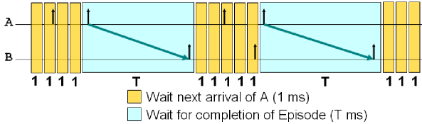
Figure 2: A schematic of the counting process for non-overlapped occurrences of the episode $A\stackrel{{\scriptstyle T}}{{\rightarrow}}B$ superimposed on the spike trains from neurons $A$ and $B$. In the yellow region there are no occurrences of the pattern starting with that time instant and the counting scheme moves forward by one time step. In the blue region there is an occurrence and the counting process moves by $T$ time steps. The random variables $X_{i}$, defined by eq. (2), capture the evolution of the counting process

Consider an episode $A\stackrel{{\scriptstyle T}}{{\rightarrow}}B$ with an inter-event time constraint (or delay) of $T$. Now, the sequence $X_{i}$ essentially captures the counting process of our algorithm. A schematic of the counting process (as relevant for this discussion) is shown in fig. 2. As explained earlier, the algorithm can be viewed as traversing a discretized time axis in steps of $\Delta T$, looking for an occurrence of the episode starting at each time instant. At each time instant (which, on the discretized time axis corresponds to an interval of length $\Delta T$), let $q_{1}$ denote the probability of spiking by $A$ and let $q_{2}$ denote the conditional probability that $B$ generates a spike $T$ instants later given that $A$ has spiked now. In terms of our earlier notation, $q_{1}=\rho_{A}$, $q_{2}=e_{s}(A,B,T)$. Thus, at any instant, $q_{1}q_{2}$ denotes the probability of occurrence of the episode starting at that instant. Now, in eq.(2) let $p=q_{1}q_{2}(=\rho_{A}e_{s}(A,B,T))$. Then $p$ represents the probability that this episode occurs starting with any given time instant. Let $L$ in eq.(3) denote the data length (in time units). Then the sequence, $X_{1},X_{2},\ldots,X_{N}$, represents our counting process. If, at the first instant there is an occurrence of the episode starting at that instant then we advance by $T$ units on the time-axis and then look for another occurrence (since we are counting non-overlapped occurrences); if there is no occurrence starting at the first instant then we advance by one unit and look for an occurrence. Also, whether or not there is an occurrence starting from the current instant is independent of how many occurrences are completed before the current instant (because we are counting only non-overlapped occurrences). So, the counting process is well captured by accumulating the $X_{i}$’s defined above till we reach the end of data. Hence $N$ captures the number of such $X_{i}$ that we accumulate because $L$ is the data length in terms of time. Since $X_{i}$ take values $1$ or $T$, the only way $\sum X_{i}$ exceeds $L$ is if the last $X_{i}$ takes value $T$ which in turn implies that when we reached end of data we have a partial occurrence of the episode. In this case the total number of completed occurrences is one less than the number of $X_{i}$ (out of $N$) that take value $T$. If the last $X_{i}$ has taken value 1 (and hence the sum is equal to $L$) then the number of completed occurrences is equal to the number of $X_{i}$ that take value $T$. Now, it is clear that $M$ is the number of non-overlapped occurrences counted.

It is easy to see that the model captures counting of episodes of arbitrary length also. For example, if our episode is $A\stackrel{{\scriptstyle T_{1}}}{{\rightarrow}}B\stackrel{{\scriptstyle T_{2}}}{{\rightarrow}}C$ then $T$ is eq.(2) would be $T_{1}+T_{2}$ and $p$ would be $\rho_{A}e_{s}(A,B,T_{1})e_{s}(B,C,T_{2})$. Suppose in a $n$-node episode the conditional probability of $j^{\mbox{th}}$ neuron firing (after the prescribed delay) given that the previous one has fired, is equal to $e_{s}^{j}$. Let the successive delays be $T_{i}$. Let the (unconditional) probability of the first neuron (of the episode) firing at any instant (that is, in any interval of length $\Delta T$) is $\rho$. Then we will take (for the $n$-node episode) $p=\rho\Pi_{j=2}^{n}(e_{s}^{j})$ and $T=\sum T_{i}$.

3.1 Mean and Variance of $M(L,T,p)$

Now, we first derive some recurrence relations to calculate the mean and variance of $M(L,T,p)$ for a given episode. Fixing an episode fixes the value of $p$ and $T$. Let $F(L,T,p)=E\>M(L,T,p)$ where $E$ denotes expectation. We can derive a recurrence relation for $F$ as follows.

$$E\>M(L,T,p) = E\>\left[\;E\>[M(L,T,p)\;|\;X_{1}]\;\right]$$

$$= E\>[M(L,T,p)\;|\;X_{1}=1](1-p)\;+\>E[M(L,T,p)\;|\;X_{1}\neq 1]p$$

$$= (1-p)E\>[M(L-1,T,p)]\>+\>p(1\>+\>E[M(L-T,T,p)])$$

In words what this says is: if the first $X_{i}$ is $1$ (which happens with probability $1-p$), then the expected number of occurrences is same as those in data of length $L-1$; on the other hand, if first $X_{i}$ is not $1$ (which happens with probability $p$) then the expected number of occurrences are 1 plus the expected number of occurrences in data of length $L-T$.

Hence our recurrence relation is:

$$F(L,T,p)=(1-p)F(L-1,T,p)+p(1+F(L-T,L,p))$$ (6)

The boundary conditions for this recurrence are:

$$F(x,y,p)=0,\ \ \mbox{if}\ \ x<y\ \ \mbox{and}\ \ \forall p.$$ (7)

Let $G(L,T,p)=E[M^{2}(L,T,p)]$. That is $G(L,T,p)$ is the second moment of $M(L,T,p)$. Using the same idea as in case of $F$ we can derive recurrence relation for $G$ as follows.

$$E\>[M^{2}(L,T,p)] = E\>\left[E\>[M^{2}(L,T,p)\;|\;X_{1}]\right]$$

$$= E\>[M^{2}(L,T,p)\;|\;X_{1}=1](1-p)\;$$

$$\ \ \ \ \ \ \ \ \ \ +\>E[M^{2}(L,T,p)\;|\;X_{1}\neq 1]p$$

$$= (1-p)E\>[M^{2}(L-1,T,p)]\>+\>pE(1\>+\>M(L-T,T,p))^{2}$$

$$= (1-p)E\>[M^{2}(L-1,T,p)]\>+$$

$$\ \ \ \ \ \ \ \ \ \ \>pE(1\>+\>M^{2}(L-T,T,p)\>+\>2M(L-T,T,p))$$

Thus we get

$$G(L,T,p)=(1-p)G(L-1,T,p)\>+\>p(1\>+\>G(L-T,T,p)\>+\>2F(L-T,T,p))$$ (9)

Solving the above, we get the second moment of $M$. Let, $V(L,T,p)$ be the variance of $M(L,T,p)$. Then we have

$$V(L,T,p)=G(L,T,p)\>-\>(F(L,T,p))^{2}$$ (10)

Once we have the mean and variance we can bound the probability that the number of non-overlapped occurrences is beyond something. For example, we can use Chebyshev inequality as

$$\mbox{Pr}\left[|M(L.T,p)-F(L,T,p)|>k\sqrt{V(L,T,p)}\right]\leq\frac{1}{k^{2}}$$ (11)

for any positive $k$. . Such bounds can be used for test of statistical significance as explained below.

3.2 Test for statistical significance

Suppose we are considering $n$-node episodes. Let the allowable Type I error for the test be $\epsilon$. Then what we need is a threshold, say, $m_{th}$ for which we have

$$\mbox{Pr}_{n}\left[f_{epi}\geq m_{th}\right]\leq\epsilon,$$ (12)

where $f_{epi}$ is the frequency of any $n$-node episode and $\mbox{Pr}_{n}$ denotes probability under the null hypothesis models.

This would imply that if we find a $n$-node episode with frequency greater than $m_{th}$ then, with $(1-\epsilon)$ confidence we can reject our null hypothesis and hence assert that the discovered episode represents ‘strong’ interactions among those neurons.

Now the above can be used for assessing statistical significance of any episode as follows. Suppose we are considering an $n$-node (serial) episode. Let the first node of this episode have event type $A$. (That is, it corresponds to neuron $A$). Let $\rho_{A}$ be the probability that $A$ will spike in any interval of length $\Delta T$. (We will fix $\Delta T$ by the time resolution being considered). Let $\epsilon$ be the prescribed confidence level. Let $k$ be such that $k^{2}\geq\frac{1}{\epsilon}$. Fix $p=\rho_{A}(e_{0})^{n-1}$. Let $T$ be the sum of all inter-event delay times in the episode. Let $L$ be the total length of data (as time span in units of $\Delta T$).

Our null hypothesis is that the conditional probability for any pair of neurons is less than $e_{0}$. Further, our random variable $M$ is such that its probability of taking higher values increases monotonically with $p$. Hence, with the above $p$, the probability of $M(L,T,p)$ being greater than any value is an upper bound on the probability of the episode frequency being greater than that value under any of the models in our null hypothesis.

Thus, a threshold for significance is $m_{th}=F(L,T,p)+k\sqrt{V(L,T,p)}$ because, from eq. (11) we have

$$\mbox{Pr}\left[M(L.T,p)\geq F(L,T,p)+k\sqrt{V(L,T,p)}\right]\leq\frac{1}{k^{2}}\leq\epsilon.$$ (13)

Though we do not have closed form expressions for $F$ and $V$, using our recurrence relations, we can calculate $F(L,T,p)$ and $V(L,T,p)$ for any given values of $L,T,p$ and hence can calculate the above threshold. The only thing unspecified for this calculation is how do we get $\rho_{A}$. We can obtain $\rho_{A}$ by either estimating the average rate of firing for this neuron from the data or from other prior knowledge.

Thus, we can use eq. (13) either for assessing the significance of a specific $n$-node episode or for fixing a threshold of any $n$-node episode in our datamining algorithm. In either case, this allows us to deduce the ‘strong connections’ (if any) in the neural system being analyzed by using our datamining method.

We can summarize the the test of significance as follows. Suppose the allowed type-I error is $\epsilon$. We choose integer $k$ such that $\epsilon<\frac{1}{k^{2}}$. Suppose we want to assess the significance of a n-node sequential pattern with the total delay being $T$ based on its count. Suppose $e_{0}$ is the bound we use in our null hypothesis. Let $L$ be the total data length in time units. Let $\rho$ be the average firing rate of the first neuron in the data. Let $p=\rho(e_{0})^{n-1}$. We calculate $F(L,T,p)$ and $V(L,T,p)$ using (6), (9) and (10). Then the pattern is declared significant if its count exceeds $F(L,T,p)+k\sqrt{V(L,T,p)}$.

We like to emphasize that the threshold frequency (count) given above for an episode to be significant (and hence represent strong interactions) is likely to be larger than that needed. This is because it is obtained through a Chebyshev bound which is often loose. Thus, for example, if we choose $e_{0}=0.4$ then some strong connections which may result in the effective conditional probability value of up to 0.5 may not satisfy the test of significance at a particular significance level. This, in general, is usual in any hypothesis testing framework. In practice, we found that we can very accurately discover all connections whose strengths in terms of the conditional probabilities are about 0.2 more than $e_{0}$ at 5% confidence level. At $\epsilon=0.05$, the threshold is about 4.5 standard deviations above the mean. In a specific application, for example, if we feel that three standard deviations above the mean is a good enough threshold, then correspondingly we will be able to discover even those connections whose effective conditional probability is only a little above $e_{0}$.

This test of significance allows us to rank order the discovered patterns. For this, we run our datamining method with different thresholds corresponding to different $e_{0}$ values. Then, by looking at the sets of episodes found at different $e_{0}$ values, we can essentially rank order the strengths of different connections in the underlying system. Since any manner of assigning numerical values to strengths of connections is bound to be somewhat arbitrary, this method of rank ordering different connections in terms of strengths can be much more useful in analyzing microcircuits.

We illustrate all these through our simulation experiments in section 4.

3.3 Extension to the model

So far in this section we have assumed that the individual delays and hence the span of an episode, $T$, to be constant. In practice, even if delay is random and varies over a small interval around $T$, the threshold we calculated earlier would be adequate. In addition to this, it is possible to extend our model to take care of some random variations in such delays.

Since we have assumed that $\Delta T$ is the time resolution at which we are working, it is reasonable to assume that the delay $T$ is actually specified in units of $\Delta T$. Then we can think of the delay as a random variable taking values in a set $\{T-J,\;T-J+1,\;\cdots,T+J\}$ where $J$ is a small (relative to T) integer. For example, suppose the delay is uniformly distributed over $\{T-1,\;T,\;T+1\}$. Now we can change our model as follows:

The $\{X_{i},\ i=1,2,\ldots\}$ will now be iid random variables with distribution

$$\mbox{Prob}[X_{i}=1] = 1-p$$

$$\mbox{Prob}[X_{i}=T-1]=\mbox{Prob}[X_{i}=T]=\mbox{Prob}[X_{i}=T+1] = \frac{p}{3}$$

where we now assume that $T>2$.

We will define $N$ as earlier by eq. (3). We will now define $Z$ as the number of $X_{i}$ out of first $N$ that do not take value 1. In terms of this $Z$, we will define $M$ as earlier by eq. (4).

Now it is easy to see that our $M(L,T,p)$ would again be the random variable corresponding to number of non-overlapped occurrences in this new scenario where there are random variations in the delays. Now the recurrence relation for $F(L,T,p)$ would become

$$F(L,T,p) = (1-p)F(L-1,T,p)+$$

$$p\left(1+\frac{1}{3}(F(L-T+1,L,p)+F(L-T,L,p)+F(L-T-1,L,p))\right)$$

The recurrence relation for variance of $M(L,T,p)$ can also be similarly derived. Now, we can easily implement the significance test as derived earlier. While the recurrence relations are a little more complicated, it makes no difference to our method of significance analysis because these recurrence relations are anyway to be solved numerically.

It is easy to see that this method can, in principle, take care of any distribution of the total delay (viewed as a random variable taking values in a finite set) by modifying the recurrence relation suitably.

4 Simulation Experiments

In this section we describe some simulation experiments to show the effectiveness of our method of statistical significance analysis. We show that our stochastic model properly captures our counting process and that the frequency threshold we calculate is effective for separating connections that are ‘strong’ (in the sense of conditional probabilities). We also show that our frequency can properly rank order the strengths of connections in terms of conditional probabilities. As a matter of fact, our results provide good justification for saying that conditional probabilities provide a very good scale for denoting connection strengths. For all our experiments we choose synthetically generated spike trains. This is because then we know the ground truth about connection strengths and hence can test the validity of our statistical theory. For the simulations we use a data generation scheme where we model the spiking of each neuron as an inhomogeneous Poisson process on which is imposed an additional constraint of refractory period. (Thus the actual spike trains are not truly Poisson even if we keep the rate fixed). The inhomogeneity in the Poisson process are due to the instantaneous firing rates being modified based on total input spikes received by a neuron through its synapses.

We have shown elsewhere [21, 29] that our datamining algorithms are very efficient in discovering interesting patterns of firings from spike trains and that we can discover patterns of more than ten neurons also. Since in this paper the focus is on statistical significance of the discovered patterns, we would not be presenting any results for showing the computational efficiency of the method.

4.1 Spike data generation

We use a simulator for generating the spike data from a network of interconnected neurons. Let $N$ denote the number of neurons in the network. The spiking of each neuron is modelled as an inhomogeneous Poisson process whose rate of firing is updated at time intervals of $\Delta T$. (We normally take $\Delta T$ to be 1ms). The neurons are interconnected by synapses and each synapse is characterized by a delay (which is in integral multiples of $\Delta T$) and a weight which is a real number. All neurons also have a refractory period. The rate of the Poisson process is varied with time as follows.

$$\lambda_{j}(k)=\frac{K_{j}}{1+\exp{(-I_{j}(k)+d_{j})}}$$ (15)

where $\lambda_{j}(k)$ is the firing rate of $j^{th}$ neuron at time $k\Delta T$, and $K_{j},d_{j}$ are two parameters. $I_{j}(k)$ is the total input into $j^{th}$ neuron at time $k\Delta T$ and it is given by

$$I_{j}(k)=\sum_{i}O_{i}(k)w_{ij}$$ (16)

where $O_{i}(k)$ is the output of $i^{th}$ neuron (as seen by the $j^{th}$ neuron) at time $k\Delta T$ and $w_{ij}$ is the weight of synapse from $i^{th}$ to $j^{th}$ neuron. $O_{i}(k)$ is taken to be the number of spikes by the $i^{th}$ neuron in the time interval $(\;(k-h_{ij}-1)\Delta T,\ (k-h_{ij})\Delta T]$ where $h_{ij}$ represents the delay (in units of $\Delta T$) for the synapse from $i$ to $j$. The parameter $K_{j}$ is chosen based on the dynamic range of firing rates that we need to span. The parameter $d_{j}$ determines the ‘background’ spiking rate, say, $\lambda_{0j}$. This is the firing rate of the $j^{th}$ neuron under zero input. After choosing a suitable value for $K_{j}$, we fix the value of $d_{j}$ based on this background firing rate specified for each neuron.

We first build a network that has many random interconnections with low weight values and a few strong interconnections with large weight values. We then generate spike data from the network and show how our method can detect all strong connections. To build the network we specify the background firing rate (which we normally keep same for all neurons) which then fixes the value of $d_{j}$ in (15). We specify all weights in terms of conditional probabilities. Given a conditional probability we first calculate the needed instantaneous firing rate so that probability of at least one spike in the $\Delta T$ interval is equal to the specified conditional probability. Then, using (15) and (16), we calculate the value of $w_{ij}$ needed so that the receiving neuron ($j$) reaches this instantaneous rate given that the sending neuron ($i$) spikes once in the appropriate interval and assuming that input into the receiving neurons from all other neurons is zero.

We note here that the background firing rate as well as the effective conditional probabilities in our system would have some small random variations. As said above, we fix $d_{j}$ so that on zero input the neuron would have the background firing rate. However, all neurons would have synapses with randomly selected other neurons and the weights of these synapses are also random. Hence, even in the absence of any strong connections, the firing rates of different neurons keep fluctuating around the background rate that is specified. Since we choose random weights from a zero mean distribution, in an expected sense we can assume the input into a neuron to be zero and hence the average rate of spiking would be the background rate specified. We also note that the way we calculate the effective weight for a given conditional probability is also approximate and we chose it for simplicity. If we specify a conditional probability for the connection from $A$ to $B$, then, the method stated in the previous paragraph fixes the weight of connection so that the probability of $B$ firing at least once in an appropriate interval given that $A$ has fired is equal to this conditional probability when all other input into $B$ is zero. But since $B$ would be getting small random input from other neurons also, the effective conditional probability would also be fluctuating around the nominal value specified. Further, even if the random weights have zero mean, the fluctuations in the conditional probability may not have zero mean due to the nonlinear sigmoidal relationship in (15). The nominal conditional probability value determines where we operate on this sigmoid curve and that determines the bias in the excursions in conditional probability for equal fluctuations in either directions in the random input into the neurons. We consider this as a noise in the system and show that our method of significance analysis is still effective.

The simulator is run as follows. First, for any neuron we fix a fraction (e.g., 25%) of all other neurons that it is connected to. The actual neurons that are connected to any neuron are then selected at random using a uniform distribution. We fix the delays and background firing rates for all neurons. We then assign random weights to connections by choosing uniformly from an interval. In our simulation experiments we specify this range in terms of conditional probabilities. For example suppose the background firing rate is 20 Hz. Then with $\Delta T=1ms$, the probability of firing in any interval of length $\Delta T$ is (approximately) 0.02. Hence a conditional probability of 0.02 would correspond to a weight value of zero. Then a range of conditional probabilities such as $[0.01,\ 0.04]$ (increase or decrease by a factor of 2 in either direction) would correspond to a weight range around zero. After fixing these random weights, we incorporate a few strong connections which vary in different simulation experiments. These weight values are also specified in terms of conditional probabilities. We then generate a spike train by simulating all the inhomogeneous Poisson processes where rates are updated every $\Delta T$ time instants. We also fix refractory period for neurons (which is same for all neurons). Once a neuron is fired, we will not let it fire till the refractory period is over.

4.2 Results

For the results reported here we used a network of 100 neurons with the nominal firing rate being 20 Hz. Each neuron is connected to 25 randomly selected neurons with the effective conditional probability of the connection strength ranging over $[0.01,\ 0.04]$. With 20Hz firing rate and 1ms time resolution, the effective conditional probability when two neurons are independent is 0.02. Thus the random connections have conditional probabilities that vary by a factor of two on either side as compared to the independent case. We then incorporated some strong connections among some neurons. For this we put in one 3-node episode, three 4-node episodes, three 5-node episodes and one 6-node episode with different strengths for the connections. The connection strengths are so chosen so that we have enough number of 3-node and 4-node episodes (as possibly subepisodes of the embedded episodes) spanning the range of conditional probabilities from 0.1 to 0.8. All synaptic connections have a delay of 5ms. Using our simulator described earlier, we generated spike trains for 20 sec of time duration (during which there are about 50,000 spikes typically), and obtained the counts of non-overlapped occurrences of episodes of all sizes using our datamining algorithms. In all results presented below, all statistics are calculated using 1000 repetitions of this simulation. Typically, on a data sequence for 20 Sec duration, the mining algorithms (run on a dual-core Pentium machine) take about a couple of minutes.

As explained earlier, in our simulator, the rate of the Poisson process (representing the spiking of a neuron) is updated every 1ms based on the actual spike inputs received by that neuron. This would, in general, imply that many pairs of neurons (especially those with strong connections) are not spiking as independent processes. Fig. 3 shows this for a few pairs of neurons. The figure shows the cross correlograms (with bin size of 1 ms and obtained using 1000 replications) for pairs of neurons that have weak connections and for pairs of neurons that have strong connections. There is a marked peakiness in the cross correlogram for neurons with strong interconnections, as expected.

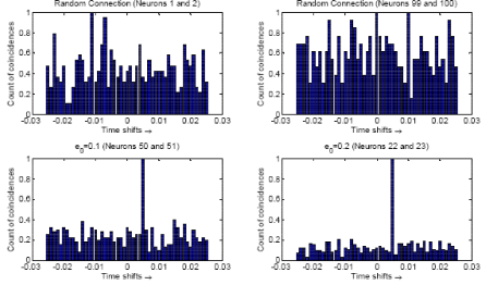
Figure 3: Normalized cross correlograms (obtained through 1000 replications) for four different pairs of neurons. The top two panels show pairs of neurons with weak interconnections while the two bottom panels show neuron pairs with strong interconnections. For neurons pairs in the bottom two panels, the cross correlogram shows strong peak.

Fig. 4 shows that our theoretical model for calculating the mean and variance of of the non-overlapped count (given by $F$ and $V$ determined through eqns. (6) and (10) ) are accurate. The figure shows plot of the mean ($F$) and mean plus three times standard deviation ($F+3\sqrt{V}$) for different values of the connection strength in terms of conditional probabilities ($e_{0}$), for the different episode sizes. Also shown are the actual counts obtained for episodes of that size with different $e_{0}$ values. As is easily seen, the theoretically calculated mean and standard deviations are very accurate. Notice that most of the observed counts are below the $F+k\sqrt{V}$ threshold for $k=3$ even though this corresponds to a Type-I error of just over 10%. Thus our statistical test with $k=3$ or $k=4$ should be quite effective.

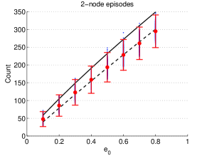
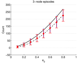
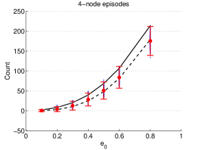
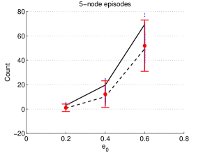
Figure 4: The analytically calculated values for the mean (i.e., $F$) and the mean plus 3 $\sigma$ (i.e., $F+3\sqrt{V}$), as a function of the connection strength in terms of conditional probabilities. The top two panels show plots for 2-node and 3-node patterns and bottom panels show plots for 4-node and 5-node patterns. For each value of the conditional probability, the actual counts as obtained by the algorithm are also shown These are obtained through 1000 replications. For these experimental counts, the mean value as well as the $\pm 3\sigma$ range (where $\sigma$ is the data standard deviation) are also indicated. As can be seen, the calculated value of $F$ well captures the mean of the non-overlapped counts. The $F+3\sqrt{V}$ line captures most of the count distribution.

As explained earlier, using the formulation of our significance test we can infer a (bound on the) connection strength in terms of conditional probability based on the observed count. For this, given observed count of a sequential pattern or episode, we ask what is the value of the strength or conditional probability of the connection at which this count is the threshold as per our significance test. This is illustrated in Fig. 5. For an $n$-node episode if the inferred strength is $q$ then we can assert (with the appropriate confidence) that it is highly unlikely for this episode to have this count if connection strength between every pair of neurons is less than $q$

In Fig. 6 we show how good is this mechanism for inferring the strength of connection. Here we plot the actual value of the strength of connection in terms of the conditional probability as used in the simulation against the inferred value of this strength from our theory based on the actual observed value of count. For each value of the conditional probability, we have 1000 replications and these various inferred values are shown as point clouds. Since the theory is based on a bound, the inferred value would always be lower than the actual strength. However, the results in this figure show the effectiveness of our approach to determining significance of sequential patterns based on counting the non-overlapped occurrences. We emphasize here that this inferred value of strength is based on our significance test and there is no estimation of any conditional probabilities.

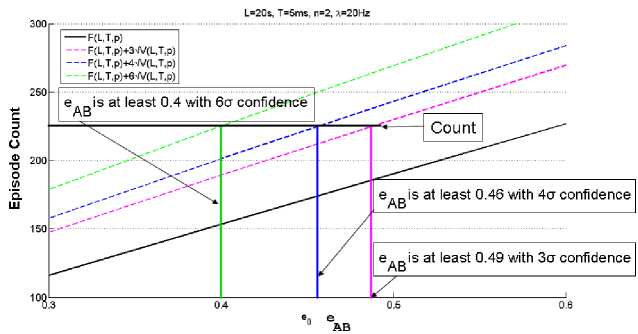
Figure 5: Illustration of inferring of a connection strength based on observed count for a pattern. Given the curves of mean $F$, and the various levels of threshold ($F+3\surd{V}$, $F+4\surd{V}$, and $F+6\surd{V}$), we can ‘invert’ the observed count to obtain a connection strength at which the observed count makes the episode just significant at a particular level. We call this the inferred connection strength based on the observed count.

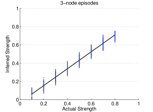
Figure 6: Plot of the actual value of the conditional probability used in simulation versus the value inferred from our test of significance as explained in text. (See fig. 5. For each value we do 1000 replications and the different inferred values are shown as a point cloud. Also shown is a best fit line. The two panels show results for episodes of size 3 and size 4. Our method is quite effective in inferring a connection strength based on our count.

Finally, we present some results to illustrate the ability of our significance test to correctly rank order different sequential patterns or episodes that are significant. For this we show the distribution of counts for sequential patterns or episodes of different strength along with the thresholds as calculated by our significance test when the value of $e_{0}$ in the null hypothesis is varied. These results are shown for 3-node, 4-node and 5-node episodes in fig. 7. From the figure we can see that, by choosing a particular $e_{0}$ value in the null hypothesis, our test will flag only episodes corresponding to strength higher than $e_{0}$ as significant. Thus, by varying $e_{0}$ we can rank-order different significant patterns that are found by the mining algorithm. We note here that our threshold actually overestimates the count needed because it is based on a loose bound. However, these results show that we can reliably infer the relative strengths of different sequential patterns.

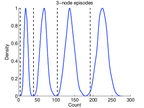
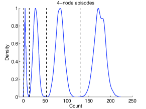
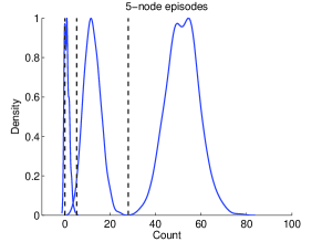
Figure 7: Plot showing the ability of our method of statistical significance test at inferring relative strengths of different patterns. Top two panel shows the distribution of counts (over 1000 replications) for four 3-node and 4-node episodes with connection strengths corresponding to 0.2, 0.4, 0.6 and 0.8. The dashed lines are the thresholds on counts under our significance test (with $k=3$) corresponding to $e_{0}$ values of 0.05, 0.25, 0.45 and 0.65. The bottom panel shows distributions for 5-node episodes with strengths 0.1, 0.3 and 0.5 with thresholds corresponding to $e_{0}$=0.05, 0.15 and 0.35. Since our test is based on Chebyshev inequality, it overestimates the needed count. However, it is easy to see that we can detect significant episodes corresponding to different strengths by varying the $e_{0}$ in our null hypothesis. As can be seen, our method is able to reliably infer the relative strengths of different patterns.

5 Discussion

In this paper we addressed the problem of detecting statistically significant sequential patterns in multi-neuronal spike train data. We employed an efficient datamining algorithm that detects all frequently occurring sequential patterns with prescribed inter-neuron delays. A pattern is frequent if the number of non-overlapping occurrences of the pattern is above a threshold. The strategy of counting only the non-overlapped occurrences rather than all occurrences makes the method computationally attractive. The main contribution of the paper is a new statistical significance test to determine when the count obtained by our algorithm is statistically significant. Or, equivalently, the method gives a threshold for different patterns so that the algorithm can detect only the significant patterns.

The novelty in assessing the significance in our approach is in the structure of the null hypothesis. The idea is to use conditional probability as a mechanism to capture strength of influence of one neuron on another. Our null hypothesis is specified in terms of a (user-chosen) bound on the conditional probability that $B$ will fire after a specified delay given that $A$ has fired, for any pair of neurons $A$ and $B$. Thus this compound null hypothesis includes many models of inter-dependent neurons where the influences among neurons are ‘weak’ in the sense that all such pairwise conditional probabilities are below the bound. Being able to reject such a null hypothesis makes a stronger case for concluding that the detected patterns represent significant functional connectivity. Equally interestingly, such a null hypothesis allows us to rank order the different patterns in terms of their strengths of influence. If we chose this bound $e_{0}$ to be the value of the conditional probability when the different neurons are independent, then we get the usual null hypothesis of independent neuron model. But since we can choose the $e_{0}$ to be much higher, we can decide which patterns are significant at different levels of $e_{0}$ and hence get an idea of the strength of interaction they represent. Thus, the method presented here extends the current techniques of significance analysis.

While we specify our null hypothesis in terms of a bound on the conditional probability, note that we are not in any way estimating such conditional probabilities. Estimating all relevant conditional probabilities would be computationally intensive. Since our algorithm counts only non-overlapped occurrences and also uses the datamining idea of counting frequencies for only the relevant candidate patterns, our counts do not give us all the pair-wise conditional probabilities. However, the statistical analysis presented here allows us to obtain thresholds on the non-overlapped occurrences possible (at the given confidence level) if all the conditional probabilities are below our bound. This is what gives us the test of significance.

We presented a method for bounding the probability that, under the null hypothesis, a pattern would have more than some number of non-overlapped occurrences. Because we are counting non-overlapped occurrences, we are able to capture our counting process in an interesting model specified in terms of sums of independent random variables. This model allowed us to get recurrence relations for mean and variance of the random variable representing our count under the null hypothesis which allowed us to get the required threshold using Chebyshev inequality. While this may be a loose bound, as shown through our simulation results, the bound we calculate is very effective.

Our method of analysis is quite general and it can be used in situations other than what we considered here. By choosing the value of $p$ in eq.(2) appropriately we can realize this generality in the model.

As an illustration of this we will briefly describe one extension of the model. In the method presented, while analyzing significance of a pattern $A\stackrel{{\scriptstyle T_{1}}}{{\rightarrow}}B\stackrel{{\scriptstyle T_{2}}}{{\rightarrow}}C$, we are assuming that firing of $C$ after $T_{2}$ given that $B$ has fired is independent of $A$ having fired earlier. That is why we have used $p=\rho_{A}(e_{0})^{2}$ while calculating our threshold. But suppose we do not want to assume this. Then we can have a null hypothesis that is specified by bounds on different conditional probabilities. Suppose $e_{2}(x,y,T)$ is the conditional probability that $y$ fires after $T$ given $x$ has fired and suppose $e_{3}(x,y,z,T_{1},T_{2})$ be the probability that $y$ fires after $T_{1}$ and $z$ fires after another $T_{2}$ given $x$ has fired. Now we specify the null hypothesis in terms of two parameters as: $e_{2}(x,y,T)<e_{02},\ \forall x,y$ and $e_{3}(x,y,z,T_{1},T_{2})<e_{03},\ \forall x,y,z$. Now for assessing significance of 3-node episodes we can use $p=\rho_{A}e_{03}$. Our method of analysis is still applicable without any modifications. Of course, now the user has to specify two bounds on different conditional probabilities and he has to have some reasons for distinguishing between the two conditional probabilities. But the main point here is that the model is fairly general and can accommodate many such extensions.

There are many other ways in which the idea presented here can be extended. Suppose we want to assess significance of synchronous firing patterns rather than sequential patterns based on the count of number of non-overlapped occurrences of the synchronous firing pattern. One possibility would be to use conditional probabilities of $A$ firing within an appropriate short time interval from $B$ in our null hypothesis and then use an appropriate expression for $p$ in our model. Another example could be that of analyzing occurrences of neuronal firing sequences that respect a pre-set order on the neurons as discussed in [25]. Suppose we want to assess the significance of count of such patterns of a fixed length. If we use our type of non-overlapped occurrences count as the statistic, then the model presented here can be used to assess the significance. Now the parameter $p$ would be the probability of occurrence of a sequence of that length (which respects the global order on the neurons) starting from any time instant. For a given null hypothesis, e.g., of independence, this would be a combinatorial problem similar to the one tackled in [25]. Once we can derive an expression for $p$ we can use our method for assessing significance.

Though we did not discuss the computational issues in this paper, the data mining algorithms used for discovering sequential patterns are computationally efficient (see [21] for details). One computational issue that may be relevant for this paper may be that of data sufficiency. All the results reported here are on spike data of 20 sec duration with background spiking rate of 20 Hz. (That works out to about 400 spikes per neuron on the average in the data). From fig. 4 we can see that, with this much of data, we can certainly distinguish between connection strengths that differ by about 0.2 on the conditional probability scale. (Notice that, in the figure, the mean plus three sigma range of the count distribution at a connection strength is below our threshold (with $k=3$) at a connection strength 0.2 more). In fig. 7 we showed that we can reliably rank order connection strengths with about the same resolution. Thus we can say that 20 sec of data is good enough for this level of discrimination. Obviously, if we need to distinguish between only widely different strengths, much less data would suffice.

In terms of computational issues, we feel that one of the important conclusions from this paper is that temporal data mining may be an attractive approach for tackling the problem of discovering firing patterns (or microcircuits) in multi-neuronal spike trains. In temporal data mining literature, episodes are, in general, partially ordered sets of event types. Here we used the methods for discovery of serial episodes which correspond to our sequential patterns. A general episode would correspond to a graph of interconnections among neurons. However, at present, there are no efficient algorithms for discovering frequently occurring graph patterns from a data stream of events. Extending our data mining algorithm and our analysis technique to tackle such graph patterns is another interesting open problem. This would allow for discovery of more general microcircuits from spike trains.

In summary, we feel that the general approach presented here has a lot of potential and it can be specialized to handle many of the data analysis needs in multi-neuronal spike train data. We would be exploring many of these issues in our future work.

Acknowledgments

We wish to thank Mr. Debprakash Patnaik and Mr. Casey Diekman for their help in preparing this paper. The simulator described here as well as the data mining package for analyzing data streams is written by Mr. Patnaik [21] and he has helped in running the simulator. Mr. Diekman has helped in generating all the figures. The work reported here is partially supported by a project funded by General Motors R&D Center, Warren through SID, Indian Institute of Science, Bangalore.

References

- [1] M Abeles. Corticonics: Neural Circuits of the Cerebral Cortex. Cambridge University Press, 1991.
- [2] M. Abeles and I. Gat. Detecting precise firing sequences in experimental data. J Neurosci Methods, 107(1-2):141–154, May 2001.
- [3] M. Abeles and G. L. Gerstein. Detecting spatiotemporal firing patterns among simultaneously recorded single neurons. J Neurophysiol, 60(3):909–924, Sep 1988.
- [4] R. Agrawal and R. Srikant. Mining sequential patterns. In Philip S. Yu and Arbee S. P. Chen, editors, Eleventh International Conference on Data Engineering, pages 3–14, Taipei, Taiwan, 1995. IEEE Computer Society Press.
- [5] A. Amarasingham. Statistical methods for the assessment of temporal structure in the activity of the nervous system. PhD thesis, Division of Applied Mathematics, Brown University, Providence, RI, USA, 2004.
- [6] D. R. Brillinger. Nerve cell spike train data analysis: a progression of thechniques. J. Am. Statist. Assoc., 87:260–271, 1992.
- [7] E. N. Brown, R. E. Kass, and P. P. Mitra. Multiple neural spike train data analysis: state-of-the-art and future challenges. Nat Neurosci, 7(5):456–461, May 2004.
- [8] A. Date, E. Bienenstock, and S. Geman. On the temporal resolution of neural activity. Technical report, Division of Applied Mathematics, Brown University, Providence, RI, USA, 1998.
- [9] J. le Feber, W. L. C. Rutten, J. Stegenga, P. S. Wolters, G. J. A. Ramakers and J. van Pelt. Conditional firing probabilities in cultured neuronal networks: a stable underlying structure in widely varying spontaneous activity patterns. J. Neural Eng., 4:54–67, 2007.
- [10] S. Fujisawa, A. Amarasingham, M. T. Harrison and G. Buzsaki. Behaviour-dependent short-term assembly dynamics in the medial prefrontal cortex. Nature Neuroscience, 2008.
- [11] G. L. Gerstein. Searching for significance in spatio-temporal firing patterns. Acta Neurobiol Exp (Wars), 64(2):203–207, 2004.
- [12] Y. Ikegaya, G. Aaron, R. Cossart, D. Aronov, I. Lampl, D. Ferster, and R. Yuste. Synfire chains and cortical songs: temporal modules of cortical activity. Science, 304(5670):559–564, Apr 2004.
- [13] E. M. Izhikevich. Polychronization: computation with spikes. Neural Computation, 18(2):245–282, Feb 2006.
- [14] R. E. Kass, V. Ventura, and E. N. Brown. Statistical issues in the analysis of neuronal data. J Neurophysiol, 94(1):8–25, Jul 2005.
- [15] S. Laxman and P. S. Sastry. A survey of temporal data mining. SADHANA, Academy Proceedings in Engineering Sciences, 2005.
- [16] S. Laxman, P. S. Sastry, and K. P. Unnikrishnan. Discovering frequent episodes and learning hidden markov models: A formal connection. IEEE Transactions on Knowledge and Data Engineering, 17(11):1505–1517, 2005.
- [17] S. Laxman, P. S. Sastry, and K. P. Unnikrishnan. A fast algorithm for finding frequent episodes in event streams. In Proc. ACM SIGKDD Int. Conf. Knowledge Discovery and Datamining, San Jose, USA, August 2007.
- [18] A. K. Lee and M. A. Wilson. Memory of sequential experience in the hippocampus during slow wave sleep. Neuron, 36(6):1183–1194, Dec 2002.
- [19] A. K. Lee and M. A. Wilson. A combinatorial method for analyzing sequential firing patterns involvingan arbitrary number of neurons based on relative time order. J Neurophysiol, 92(4):2555–2573, 2004.
- [20] F. Morchen. Unsupervised pattern mining from symbolic temporal data. SIGKDD Explorations, 9:41–55, 2007.
- [21] D. Patnaik, P. S. Sastry and K. P. Unnikrishnan. Inferring neuronal network connectivity from spike data: A temporal datamining approach. Scientific Programming (Special issue on Biological Data Mining), 16(1):49–77, 2008.
- [22] G. Pipa, D. W. Wheeler, W. Singer and D. Nikolic. NeuroXidence: Reliable and efficient analysis of an excess or deficiency of joint spike events. J. Computational Neuroscience, 25(1):64-88, 2008.
- [23] F. Rigat, M. Gunst, and J. Pelt. Bayesian modelling and analysis of spatio-temporal neuronal networks. Bayesian Analysis, 1(4):733–764, 2006.
- [24] T. Sasaki, N. Matsuki and Y. Ikegaya. Metastability of active CA3 networks. The Journal of Neuroscience, 27(3):517–528, 2007.
- [25] A. C. Smith and P. Smith. A set probability technique for detecting relative time order across multiple neurons. Neural Computation, 18:1197–1214, 2006.
- [26] I. V. Tetko and A. E. Villa. A pattern grouping algorithm for analysis of spatiotemporal patterns in neuronal spike trains: I. detection of repeated patterns. J Neurosci Methods, 105(1):1–14, Jan 2001.
- [27] M. Meister. Multineuronal codes in retinal signaling. Proc Natl Acad Sci U S A, 93(2):609–614, Jan 1996.
- [28] I. V. Tetko and A. E. Villa. A pattern grouping algorithm for analysis of spatiotemporal patterns in neuronal spike trains: I. detection of repeated patterns. J Neurosci Methods, 105(1):1–14, Jan 2001.
- [29] K. P. Unnikrishnan, D. Patnaik, and P. S. Sastry. Discovering patterns in multi-neuronal spike trains using the frequent episode method. Technical report, 2007. available at http://www.citebase.org/abstract?id=oai:arXiv.org:0709.0566.
- [30] D. A. Wagenaar, J. Pine, and S. M. Potter. An extremely rich repertoire of bursting patterns during the development of cortical cultures. BMC Neurosci, 7:11–11, 2006.
- [31] Z. Nádasdy, H. Hirase, A. Czurkó, J. Csicsvari, and G. Buzsáki. Replay and time compression of recurring spike sequences in the hippocampus. J. Neurosci, 19:9497–9507, 1999.