The Comprehensive Analysis of Neutrino Events Occurring inside the Detector in the Super-Kamiokande Experiment from the View Point of the Numerical Computer Experiments: Part 3
– L/E Analysis for Single Ring Muon Events II –

Abstract

Following $L_{\nu}/E_{\nu}$ analysis in the preceding paper of the Fully Contained Muon Events resulting from the quasi-elastic scattering obtained from our numerical computer experiment. In the present paper, we carry out the analyses of $L_{\nu}/E_{\mu}$, $L_{\mu}/E_{\nu}$ and $L_{\mu}/E_{\mu}$ among four possible combinations of L and E. As the result of it, we show that we can not find the characteristis of maximum oscillation for neutrino oscillation among two of three, $L_{\mu}/E_{\mu}$ and $L_{\mu}/E_{\nu}$. Only $L_{\nu}/E_{\mu}$ distribution can show something like maximum oscillation, however it cannot be detected owing to the neutral character of $L_{\nu}$. It is, thus, concluded that the Super-Kamiokande Experiment could not have found the existence of the maximum oscillation for neutrino oscillation.

Keywords: Super-Kamiokande Experiment, QEL, Numerical Computer Experiment

1 Introduction

In a previous paper [1], we have carried out the $L_{\nu}/E_{\nu}$ analysis, for Fully Contained Muon Events resulting from the quasi elastic scattering(QEL)[2] obtained from our numerical experiments, namely, the most clear cut analysis for the maximum oscillation and have shown the existence of the maximum oscillations under the neutrino oscillation parameters obtained by the Super-Kamiokande Collaboration. This fact denotes that our numerical computer experiment has been performed in right way. The maximum oscillations for the neutrino oscillation are derived from the survival probability of a given flavor, such as, $\nu_{\mu}$, and it is given by

$$P(\nu_{\mu}\rightarrow\nu_{\mu})=1-sin^{2}2\theta sin^{2}(1.27\Delta m^{2}L_{\nu}/E_{\nu}).$$ (1)

However, as both $L_{\nu}$ and $E_{\nu}$ are not physically measurable quantities which are attributed to the nature of neutrino and, consequently, the maximum oscillations can not be detected through analysis of $L_{\nu}/E_{\nu}$ distribution, even if they really exist. In our numerical computer experiment, we can examine another possible combinations of L/E, such as $L_{\nu}/E_{\mu}$, $L_{\mu}/E_{\nu}$ and $L_{\mu}/E_{\mu}$ besides $L_{\nu}/E_{\nu}$. Therefore, we try to examine weather the existence of the maximum oscillation can be detected through the analysis of L/E besides $L_{\nu}/E_{\nu}$.

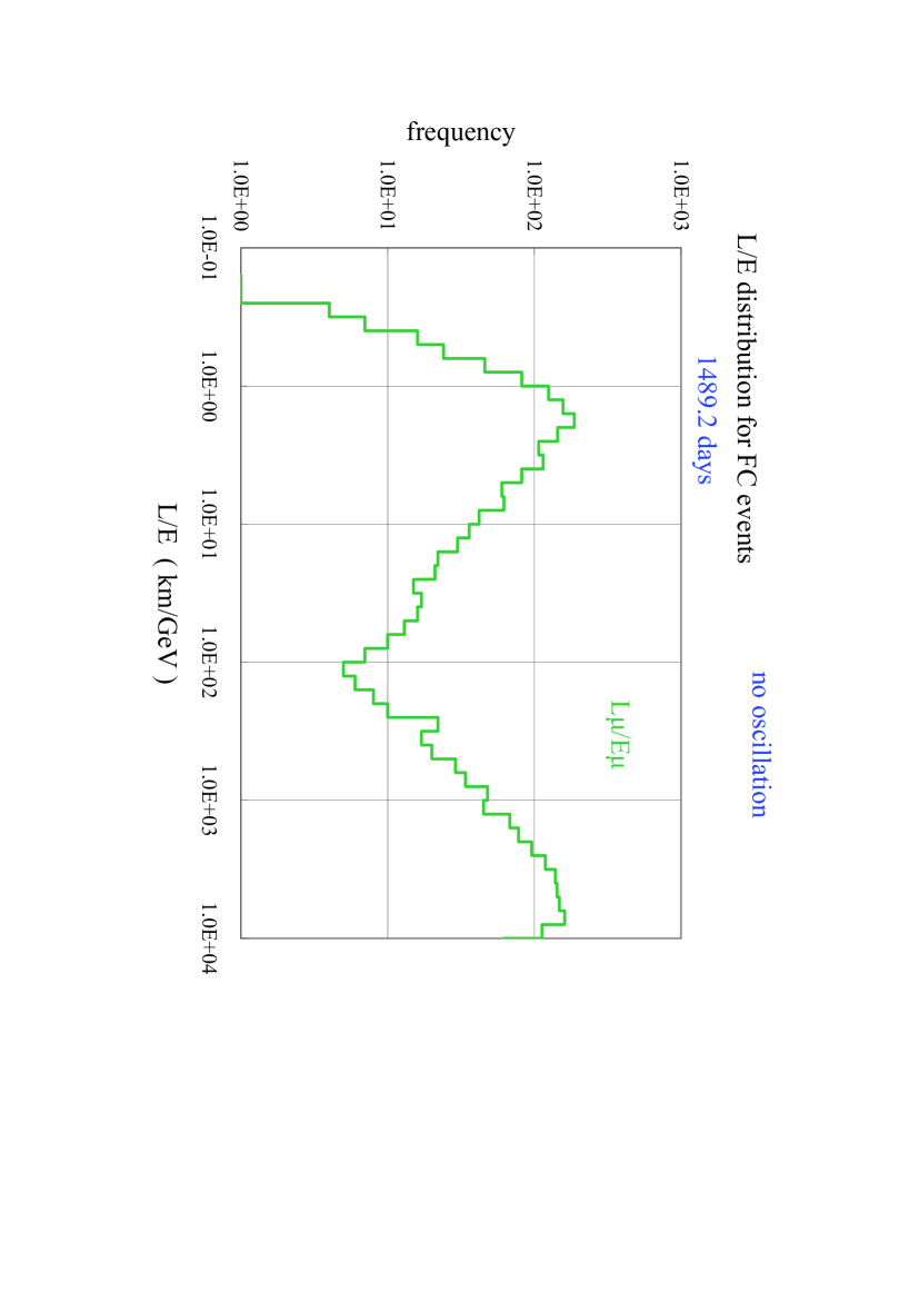
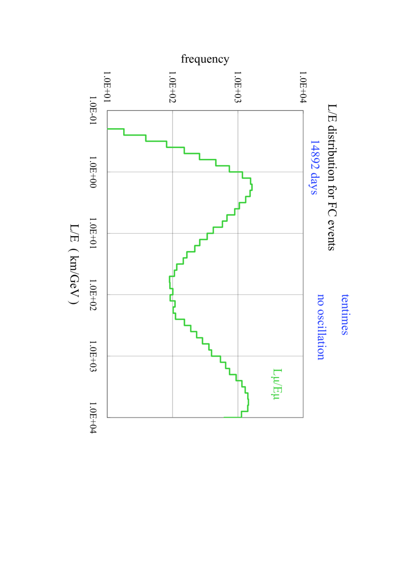
Figure 1: $L_{\mu}/E_{\mu}$ distribution without oscillation for 1489.2 live days.

Figure 2: $L_{\mu}/E_{\mu}$ distribution without oscillation for 14892 live days.

2 $L_{\mu}/E_{\mu}$, $L_{\mu}/E_{\nu}$ and $L_{\nu}/E_{\mu}$ Distributions in Our Numerical Experiment

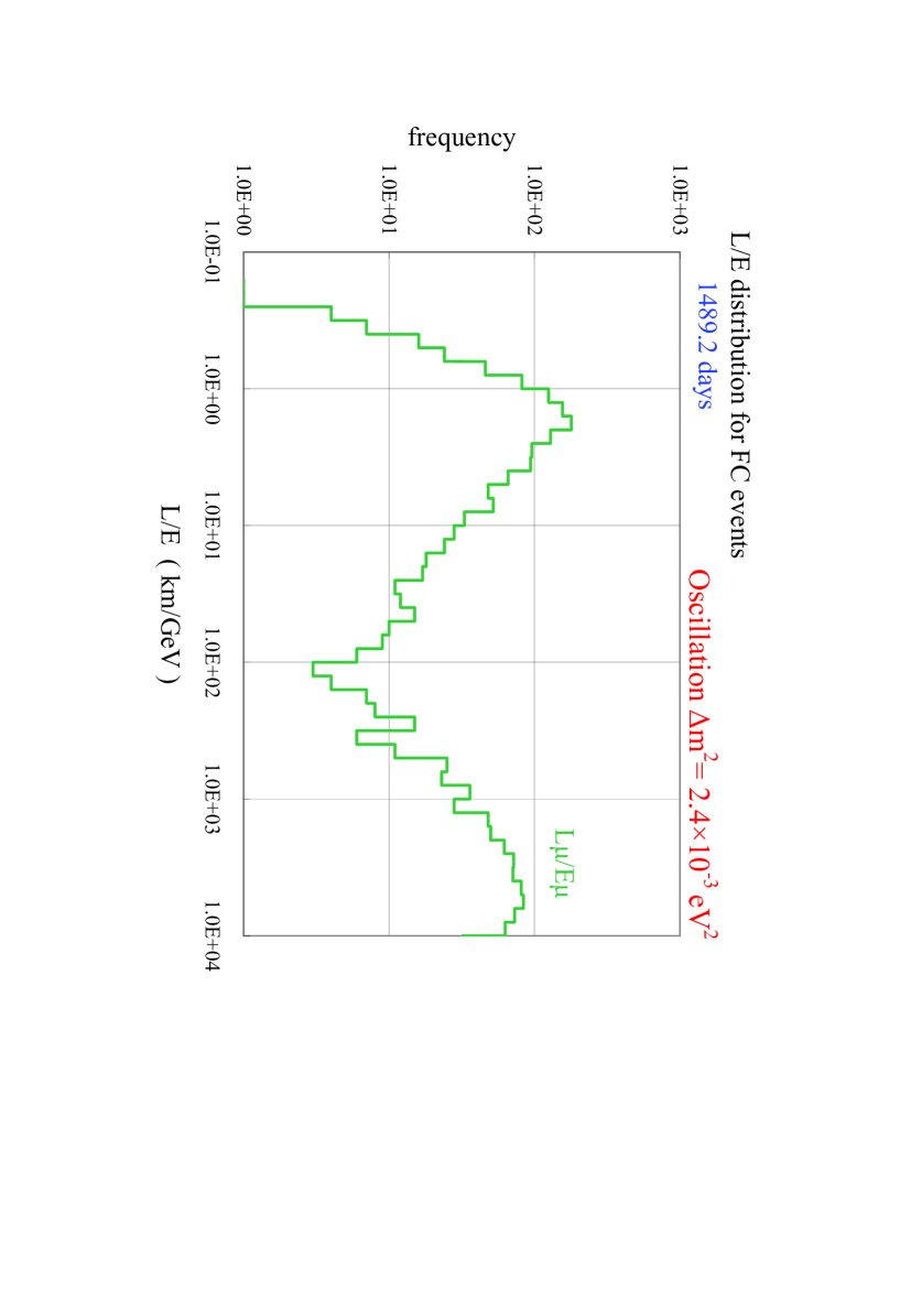
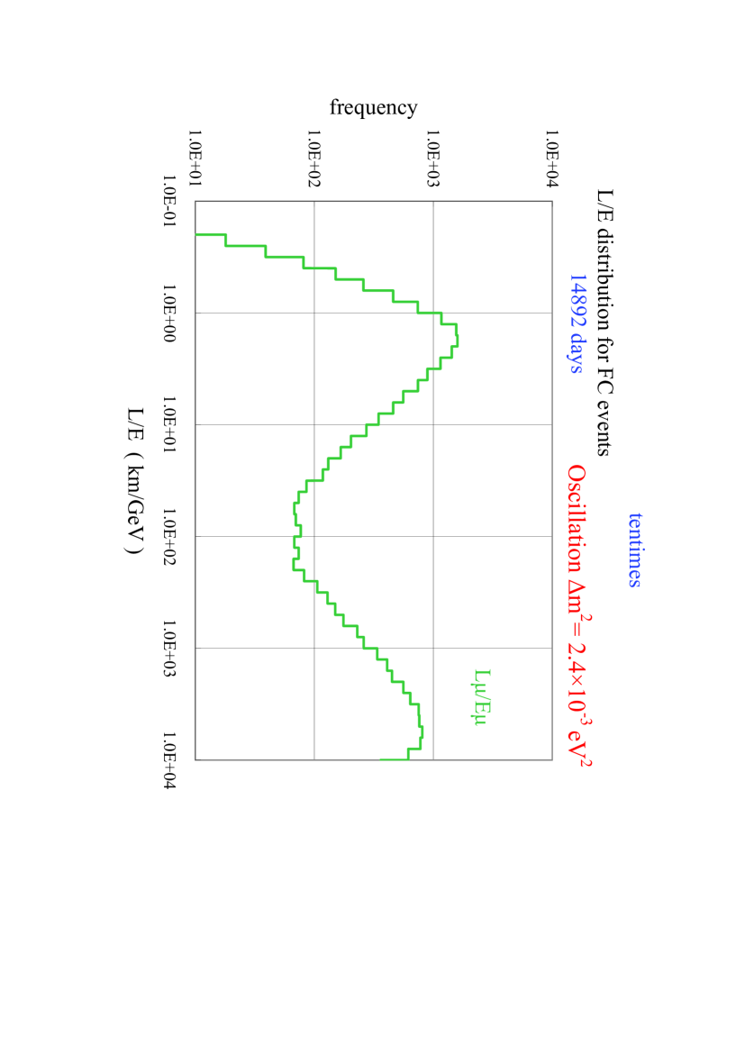
Figure 3: $L_{\mu}/E_{\mu}$ distribution with the oscillation for 1489.2 live days.

Figure 4: $L_{\mu}/E_{\mu}$ distribution with the oscillation for 14892 live days.

2.1 $L_{\mu}/E_{\mu}$ Distribution

As physical quantities which can really be observed are $L_{\mu}$ and $E_{\mu}$ instead of $L_{\nu}$ and $E_{\nu}$, therefore we examine $L_{\mu}/E_{\mu}$ distribution.

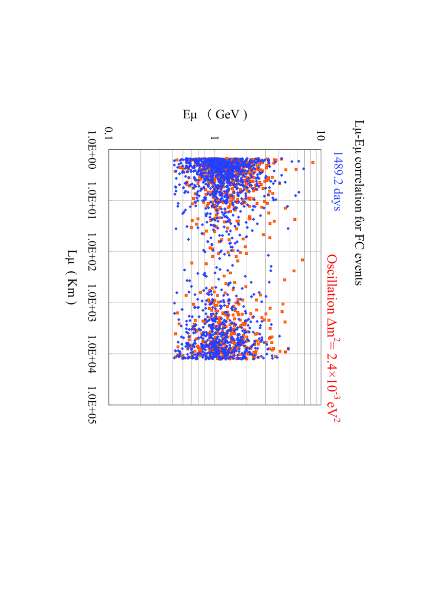
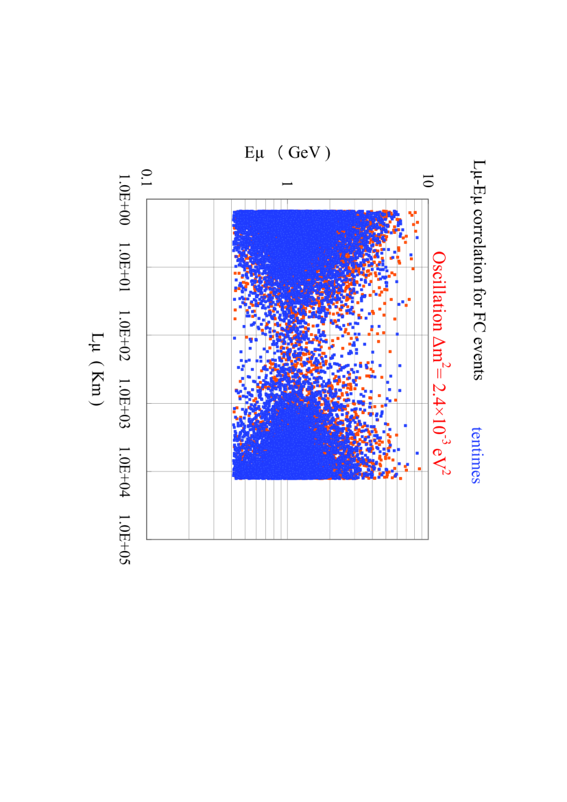
Figure 5: The correlation diagram between $L_{\mu}$ and $E_{\mu}$ with oscillation for 1489.2 live days.

Figure 6: The correlation diagram between $L_{\mu}$ and $E_{\mu}$ with oscillation for 14892 live days.

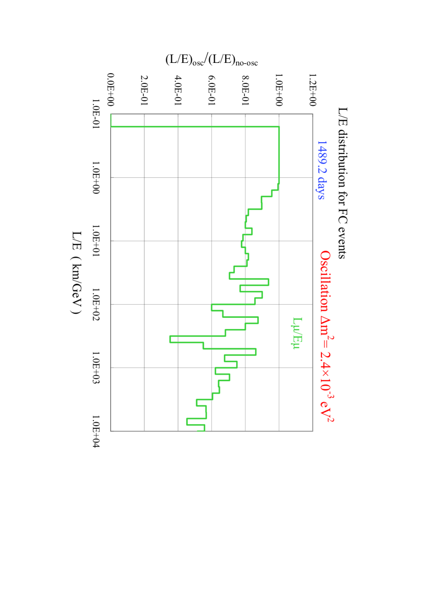
Figure 7: The ratio of $(L_{\mu}/E_{\mu})_{osc}/(L_{\mu}/E_{\mu})_{null}$ for 1489.2 live days.

Figure 8: The ratio of $(L_{\mu}/E_{\mu})_{osc}/(L_{\mu}/E_{\mu})_{null}$ for 14892 live days.

2.1.1 For null oscillation

In Figures 1 and 2, we give the $L_{\mu}/E_{\mu}$ distributions without oscillation for 1489.2 live days which is equal to the actual live days of the Super-Kamiokande Experiment[3] and 14892 live days, ten times as much as that of Super-Kamiokande Experiment, respectively. Similarly, Figures 1 and 2 show sinusoidal-like character as in Figures 6 and 7 for $L_{\nu}/E_{\nu}$ in the preceeding paper[1] which has no relation with the oscillation, however. Such the sinusoidal character represents the intersection effect due to the horizontal-like incident neutrino, partly the upward neutrinos and partly the downward neutrinos. Comparing Figure 1 with Figure 2, the characteristics of the uneven histogram in Figure 1 disappear in Figure 2 due to ten times statistics as much as that of the Figure 1.

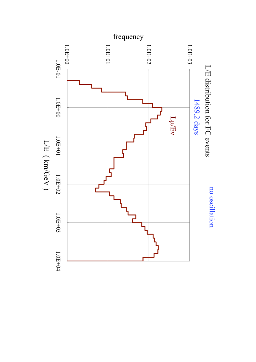
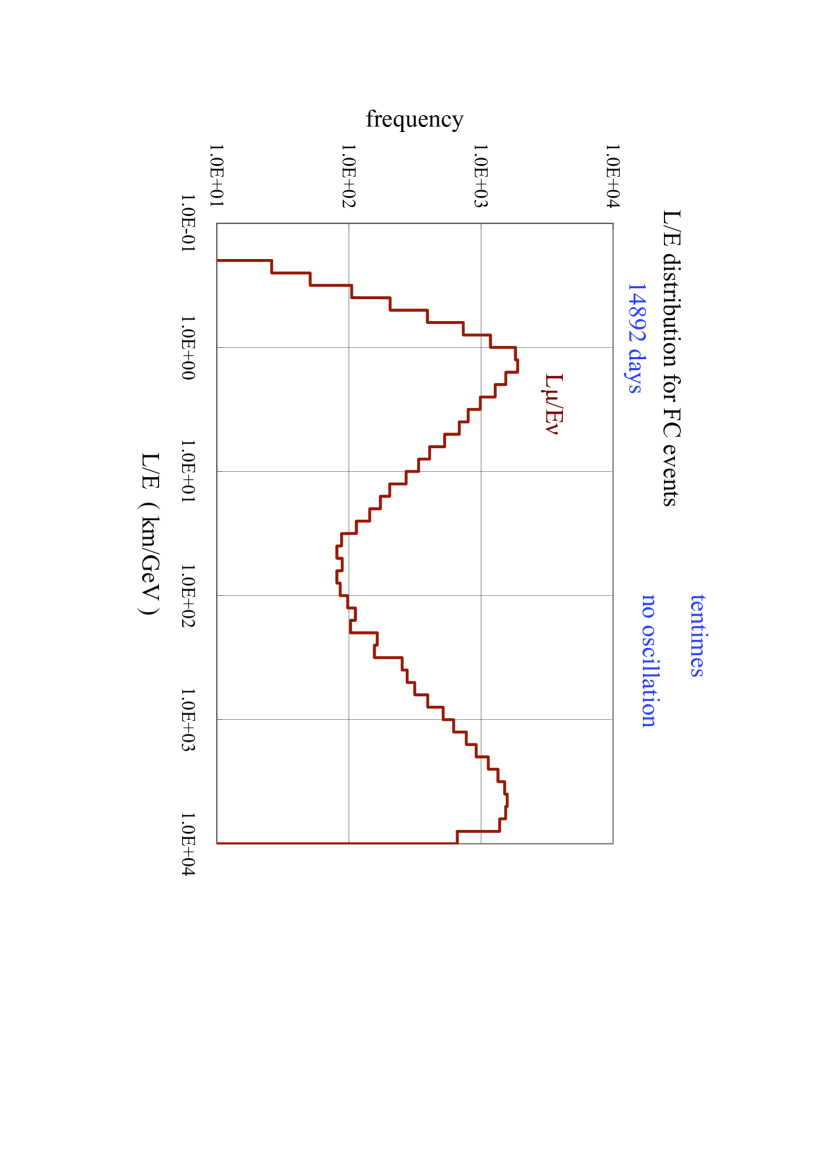
Figure 9: $L_{\mu}/E_{\nu}$ distribution without oscillation for 1489.2 live days.

Figure 10: $L_{\mu}/E_{\nu}$ distribution without oscillation for 14892 live days.

2.1.2 For the oscillation

In Figures 3 and 4, we give the $L_{\mu}/E_{\mu}$ distributions with the oscillation for 1489.2 live days and 14892 live days, respectively. In Figure 3, we may observe the uneven histogram, something like dips coming from neutrino oscillation. However, in Figure 4 where the statistics is ten times as much as that of Figure 1, the histogram becomes smoother and such the dips disappear, which turns out finally for the dips to be pseudo. Furthermore, comparing Figure 4 in the presence of neutrino oscillation with Figure 2 in the absence of neutrino oscillation, it is clear that the dips which show maximum oscillation in the Figure 10 in the preceeding paper[1] are lost in the Figure 4 under cover of the complicated relation between $L_{\nu}$ and $L_{\mu}$. It is impossible to extract the neutrino oscillation parameters from the comparison of Figure 4 with Figure 2.
In Figures 5 and 6, correspondingly, we give the correlation between $L_{\mu}$ and $E_{\mu}$ for 1489.2 live days and 14892 live days, respectively. It is clear from the figures that we can not observe any combination of $L_{\mu}/E_{\mu}$ which gives the maximum oscillation on the contrary to Figures 11 and 12 in the preceeding paper[1]. Namely, we may conclude that we can not observe the sinusoidal flavor transition probability of neutrino oscillation against the claim by the Super-Kamiokande Collaboration[4] when we adopt physically observable quantities, such as $L_{\mu}$ and $E_{\mu}$.

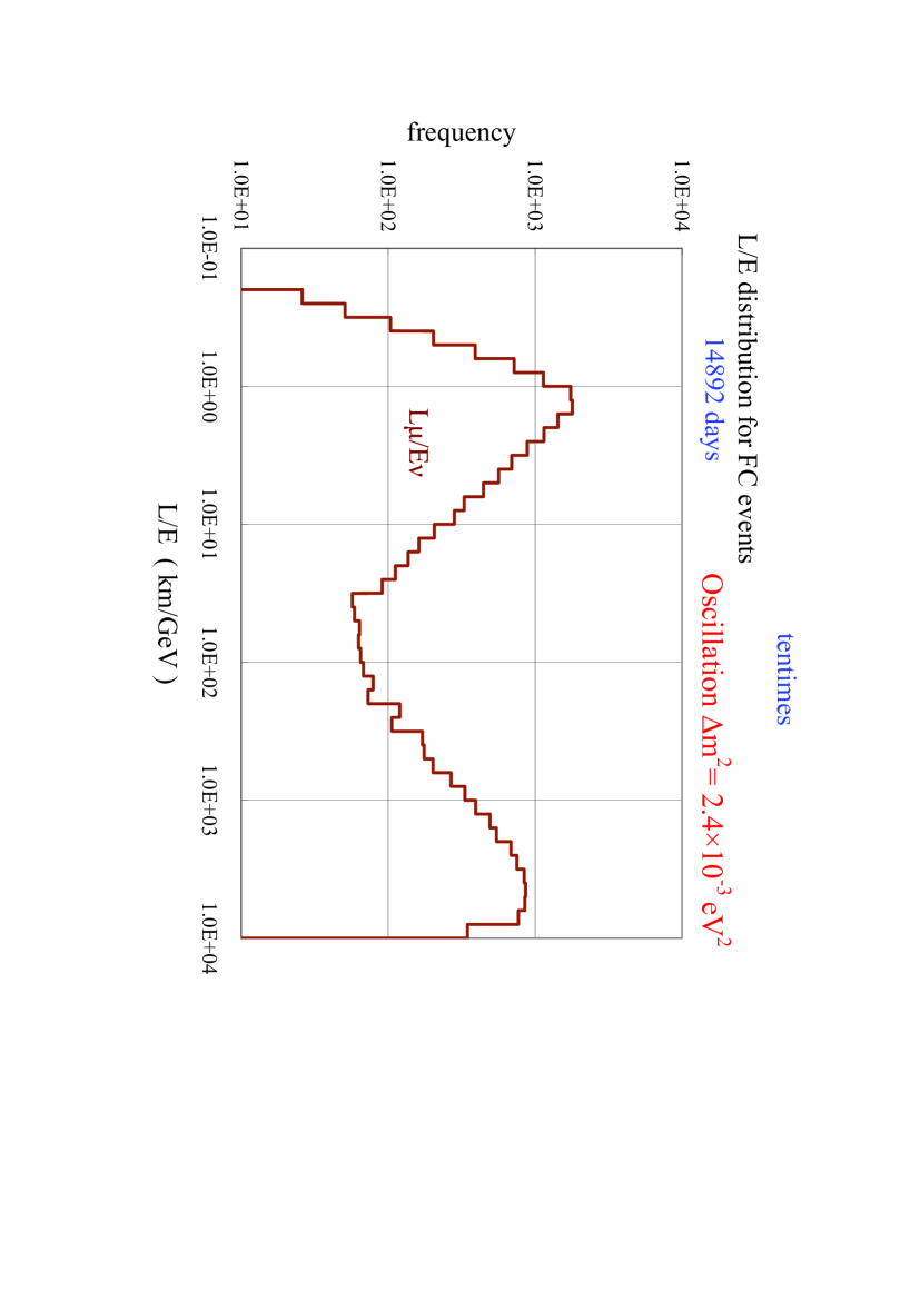
Figure 11: $L_{\mu}/E_{\nu}$ distribution with the oscillation for 1489.2 live days.

Figure 12: $L_{\mu}/E_{\nu}$ distribution with the oscillation for 14892 live days.

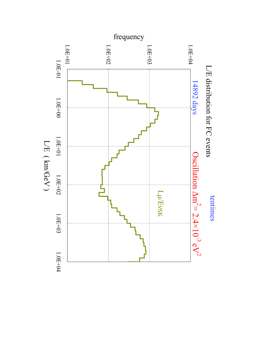
Figure 13: The $L_{\mu}/E_{\nu,SK}$ distribution with oscillation for 14892 day.

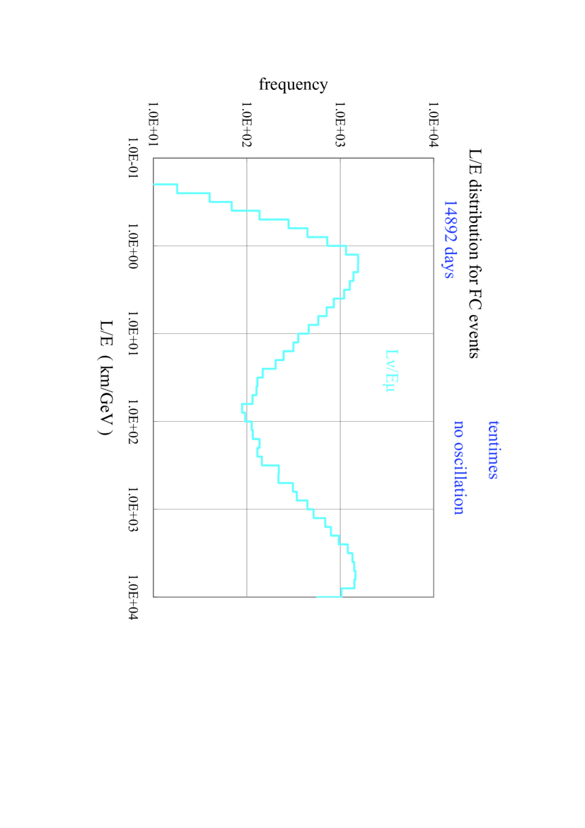
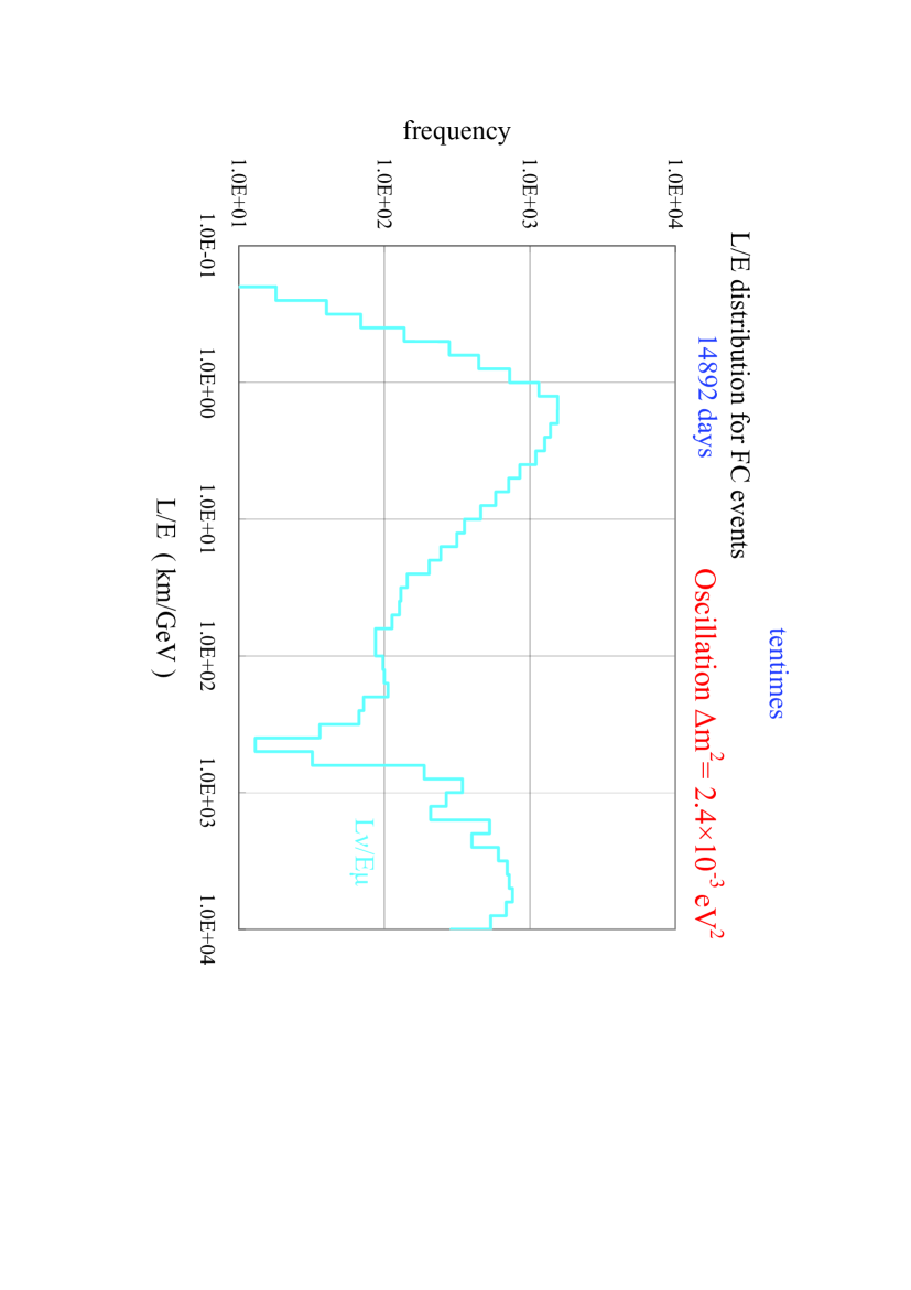
Figure 14: The $L_{\nu}/E_{\mu}$ distribution without oscillation for 14892 days.

Figure 15: The $L_{\nu}/E_{\mu}$ distribution with the oscillation for 14892 days.

In order to confirm the disappearance of the psuedo maximum oscillations, in Figures 7 and 8, we give the survival probability of a given flavor for $L_{\mu}/E_{\mu}$ distribution, namely,
$(L_{\mu}/E_{\mu})_{osc}/(L_{\mu}/E_{\mu})_{null}$, for 1489.2 live days and 14892 live days, respectively. Comparing Figure 7 with Figure 8, pseudo dips in Figure 7 disappear in Figure 8. Thus the histogram becomes a rather decreasing function of $L_{\mu}/E_{\mu}$ in Figure 8. If we further make statistics higher, the survival probability for $L_{\mu}/E_{\mu}$ distribution should be a monotonously decreasing function of $L_{\mu}/E_{\mu}$, whithout showing any characteristics of the maximum oscillation, which is contrast to Figures 8, 9 and 10 in the preceeding paper[1]. In conclusion, we should say that we can not find any maximum oscillation for the neutrino oscillation in the $L_{\mu}/E_{\mu}$ distribution.

2.2 $L_{\mu}/E_{\nu}$ Distribution

Now, we examine the $L_{\mu}/E_{\nu}$ distribution which the Super-Kamiokande Collaboration treat in the thier paper, expecting the evidence for the oscillatory signatuture in atmospheric neutrino oscillations.

2.2.1 For null oscillation

In Figures 9 and 10, we give the $L_{\mu}/E_{\nu}$ distribution without oscillation for 1489.2 live days and 14892 live days, respectively. Comparing Figure 9 with Figure 10, the larger statistics makes the distribution more smooth. Also, there is sinusoidal-like dip which have no relation with neutrino oscillation.

2.2.2 For the oscillation

In Figures 11 and 12, we give the $L_{\mu}/E_{\nu}$ distribution with oscillation for 1489.2 live days and 14892 live days, respectively. In Figure 11, we may find something like dip which corresponds to the first maximum oscillation near $\sim$200 (km/GeV). However, such the dip disappears, by making the statistics larger as shown in Figure 12. Instead, Figure 12 gives the histogram with a little unnatural shape in spite of larger statistics. This may come from the complicated correlation between $L_{\mu}$ and $E_{\nu}$, the details of which are shown partially in Eq.(2), Eq.(3) and Figure 5 in the preceeding paper[1].

2.2.3 $L_{\mu}/E_{\nu,SK}$Didtribution for the oscillation

Instead of $E_{\nu}$ which is correctly sampled from the corresponding probability functions, let us utilize $E_{\nu,SK}$ which is obtained from the ”approximate” formula (Eq.(4) in the preceeding paper[1]). We express $E_{\nu}$ described in Eq.(4) in the preceeding paper[1] utilized by the Super-Kamiokande Collaboration as $E_{\nu,SK}$ to discriminate our $E_{\nu}$ obtained in stochastic manner correctly. In Figure 13, we give $L_{\mu}/E_{\nu,SK}$ distribution for 14892 live days and 14892 live days, ten times as much as the Super-Kamiokande Experiment actual live days. . If we compare Figure 13 with Figure 12, we understand that there are no significant difference between them. This fact tells us that the ”aproximate” formula for $E_{\nu}$ by the Super-Kamiokande Collaboration, which is not suitable for the treatment of the stochastic quantities, does not produce so significant error actually, which is understandable from Figure 5 in the preceeding paper[1]. Also, we can conclude that we do not find any dip corresponding to any maximum oscillation from $L_{\mu}/E_{\nu}$ or $L_{\mu}/E_{\nu,SK}$ distributions. The reason why the Figures 10 and 13 can not show any dip structure, which is shown in Figures from 8 to 10 in the preceeding paper[1] clearly, comes from the situation that the role of $L_{\nu}$ is much more crucial than that of $E_{\nu}$ in the $L/E$ analysis. Namely, $L_{\nu}$ cannot be replaced by $L_{\mu}$ at all. Also, see the discussion in the following subsection 2.3.

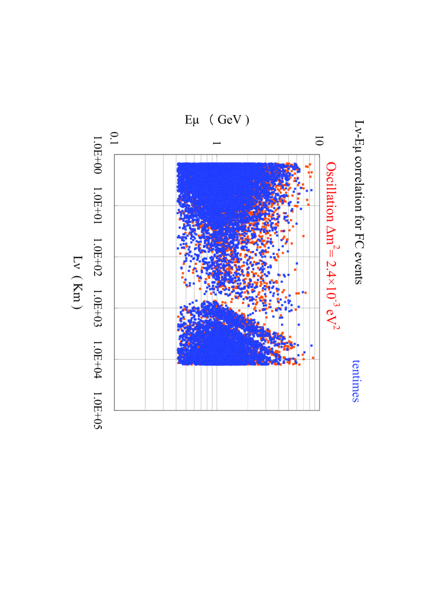
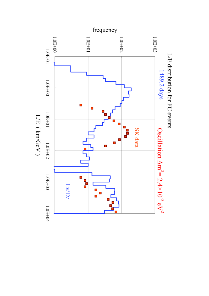
Figure 16: The correlation diagram between $L_{\nu}$ and $E_{\mu}$ with the oscillation for 14892 days.

Figure 17: The comparison of $L/E$ distribution for single-ring muon events due to QEL among Fully Contained Events with the corresponding one by the Super-Kamiokande Experiment.

2.3 $L_{\nu}/E_{\mu}$ Distribution

2.3.1 For null oscillation

In Figure 14, we give $L_{\nu}/E_{\mu}$ distribution without oscillation for 14892 days, ten times as much as actual live days of the Super-Kamiokande Experiment to consider statistical fluctuation effect as precisely as possible. It is clear from the figure that there is not any dip corresponding to the maximum oscillation which is expected to appear in the presence of the neutrino oscillation.

2.3.2 For the oscillation

In Figure 15, we give the corresponding distribution with the oscillation. In Figure 16, we give the correlation diagram between $L_{\nu}$ and $E_{\mu}$which correspond to Figure 15. On the contrary to Figure 14, there are surely dips in Figure 15, and furthermore we can discriminate the strip pattern in Figure 16, similarly as in the Figure 12 in the preceeding paper[1].

Therefore, we suppose from Figures 15 and 16 that we may observe some quantities which is directly related to the maximum oscillations in the $L_{\nu}/E_{\nu}$ distribution. However, it seems to be difficult to extract a pair of concrete values of $L_{\nu}$ and $E_{\nu}$ through the analysis of $L_{\nu}/E_{\mu}$ distribution. Comparing Figure 4 with Figure 5 in the preceeding paper[1], it is clear that $L_{\nu}$ can not be approximated by $L_{\mu}$ at all, while $E_{\nu}$ can be approximated by $E_{\mu}$ within some allowance (see Figure 5 in the preceeding paper[1] ). Thus, the $L_{\nu}/E_{\mu}$ distribution can show some similar structure to $L_{\nu}/E_{\nu}$ distribution. This fact shows that the role of $L_{\nu}$ is essentially important compared with $E_{\nu}$ in the $L/E$ analysis. However, it should be noticed again that we can not observe the $L_{\nu}/E_{\mu}$ distribution physically even if the dips surely exist in this distribution, because $L_{\nu}$ is the physically unobservable quantity.

3 Comparison of distribution from the Super-Kamiokande Experiment with our results

As the Super-Kamiokande Collaboration think that they can approximate $L_{\mu}$ nearly equal to $L_{\nu}$ and $E_{\nu}$ is well approximated by Eq.(4), their experimental data should be compared with our $L_{\nu}/E_{\nu}$ distribution.
In Figure 17, we compare our numerical experimental data for Fully Contained Events due to QEL with the corresponding one by the Super-Kamiokande Experiment (read from Figure 8.22 [5]). In the light of the correct distribution, uncertainties in the distribution from the Super-Kamiokande Experiment consist of uncertainty in $L_{\mu}$ (see Figure 4 and Eq.(3) in the preceeding paper[1]) and in the transformation of $E_{\nu}$ from $E_{\mu}$ (see Figure 5 in the preceeding paper[1]). There are big differences between our distribution and the corresponding one from the Super-Kamiokande Experiment. The first is the difference in the shape of the distribution and the second is in their dip structure. It seems to be curious that there exists a rather wider dip from 100 to 630 km/GeV for the first maximum oscillation in the distribution from the Super-Kamiokande Experiment, which is against the sense of maximum oscillation, while we give a sharp dip for the first maximum oscillation around 520 km/GeV predicted by the neutrino oscillation parameters from the Super-Kamiokande Collabolation. In order to clarify the reason for the remarkable difference between ours and that of the Super-Kamiokande Experiment, it is required that the Super-Kamiokande Collaboration disclose their correlation diagram between $L_{\nu}$ and $E_{\nu}$ as shown in Figure 12 in the preceeding paper[1].

4 Conclusion

The Super-Kamiokande Collabolation trys to get the evidence for an oscillatory signature in atmospheric neutrino oscillations by detecting the maximum oscillations (the first maximum oscillation). Then, they approximate $L_{\nu}$ by $L_{\mu}$ and estimate $E_{\nu}$ from $E_{\mu}$ in their $L/E$ analysis. However, we show that the approximation of $L_{\nu}$ by $L_{\mu}$ doest not hold at all (Figures 3 and 4 in the present paper) and the estimation method by the Super-Kamiokande Collabolation in energy is theoretically unsuitable (Figure 5 in the preceeding paper[1]). Then, it is clarified that the role of $L_{\nu}$ is more decisively cruisial than that of $E_{\nu}$ in the $L/E$ analysis. As a result of it, one can not replace $L_{\nu}/E_{\nu}$ by $L_{\mu}/E_{\nu}$.

In the $L/E$ analysis, we examine all possible combinations of $L/E$, namely, $L_{\nu}/E_{\nu}$[1], $L_{\nu}/E_{\mu}$, $L_{\mu}/E_{\nu}$ and $L_{\mu}/E_{\mu}$ in the present paper. Among all possible $L/E$ analysis, we find only the $L_{\nu}/E_{\nu}$ distribution can give the maximum oscillations from the survival probability of a given flavor (Eq. 1)), as it must be. However, the $L_{\nu}/E_{\nu}$ distribution can not be physically observed. Even if we put aside the unsuitable estimation of $E_{\nu}$ from $E_{\mu}$ by the Super-Kamiokande Collabolation(Eq. 4 in the preceeding paper[1]), it is concluded from our analysis by the numerical computer experiment that $L_{\mu}/E_{\nu}$ distribution by the Super-Kamiokande Collabolation can not obtain the maximum oscillation from the survival probability of a given flavor. From the experimental point of view, physically measurable quantities are $L_{\mu}$ and $E_{\mu}$. Therefore, it is desirable that the Super-Kamiokande Collaboration carry out the $L_{\mu}/E_{\mu}$ analysis from which they examine whether they can really observe the maximum oscillation for neutrino oscillation or not. In this case, we are free from the uncertainty which is produced by the estimation of $E_{\nu}$ from $E_{\mu}$. However, even if the Super-Kamiokande Collabolation utilizes $E_{\mu}$ instead of $E_{\nu}$, we can not observe the maximum oscillation in the $L_{\mu}/E_{\mu}$ analysis, which are shown in Figure 8.

Furthermore, it should be emphasized that confirmation of the existence of the maximum oscillations can be carried out by the analysis on the ratio of $(L/E)_{osc}/(L/E)_{null}$, but not by that of the $(L/E)_{osc}$ only. For the purpose, we should say the numerical computer experiment is an indispensable mean. In conclusion, we would say that we can not observe any maximum oscillations with the Super-Kamiokande Experiment $L/E$ analysis against the original claim by the Super-Kamiokande Collabolation.

References

References

- [1] Konishi,E.,Minorikawa,Y.,Galkin,V.I.,Ishiwata,M., Nakamura,I.,Kato,M. and Misaki,A arXiv:hep-ex/0808.3313v1
- [2] Renton, P., Electro-weak Interaction, Cambridge University Press (1990). See p. 405.
- [3] Ashie,Y et al., Phys.Rev.D171(2005)112005
- [4] Ashie,Y et al., Phys.Rev.Lett.93(2004)101801-1
- [5] Ishitsuka, M., PhD thesis, University of Tokyo (2004). See p. 138.