Generalizing the Tomboulis-Yaffe Inequality to SU(N)𝑆𝑈𝑁SU(N) Lattice Gauge Theories and General Classical Spin Systems

Takuya Kanazawa
Department of Physics, University of Tokyo, Tokyo 113-0033, Japan
Email: tkanazawa@nt.phys.s.u-tokyo.ac.jp
Abstract

We extend the inequality of Tomboulis and Yaffe in SU(2)𝑆𝑈2SU(2) lattice gauge theory (LGT) to SU(N)𝑆𝑈𝑁SU(N) LGT and to general classical spin systems, by use of reflection positivity. Basically the inequalities guarantee that a system in a box that is sufficiently insensitive to boundary conditions has a non-zero mass gap. We explicitly illustrate the theorem in some solvable models. Strong coupling expansion is then utilized to discuss some aspects of the theorem. Finally a conjecture for exact expression to the off-axis mass gap of the triangular Ising model is presented. The validity of the conjecture is tested in multiple ways.
     PACS: 05.50.+q, 11.15.Ha, 12.38.Aw, 75.10.Hk
     Key words: lattice gauge theory, vortex free energy, classical spin model, mass gap

TKYNT-08-13

1 Introduction

In this paper we generalize the inequality proved originally by Tomboulis and Yaffe in SU(2)𝑆𝑈2SU(2) gauge theories [1] to SU(N)𝑆𝑈𝑁SU(N) gauge theories with general N𝑁N and also to a wide range of classical spin systems. To make this paper readable for those working on spin systems, we give in this section an elementary introduction to studies of quark confinement in lattice gauge theories (LGT) with an emphasis on interrelations between concepts in spin systems and those in gauge theories.

That a specific kind of defect could be responsible for determining a phase structure of a statistical system is appreciated as a quite useful idea in wide areas of modern physics. It has a long history, possibly dating back to R. Peierls’ argument on the Ising model [2]. In as early as 1944 L. Onsager, in his famous paper on the exact solution of the two-dimensional square Ising model, calculated what he called a ‘boundary tension’ (the free energy per unit length of a domain wall separating two regions of opposite magnetic order) and found that it is zero above and nonzero below the critical temperature [3]; hence magnetization is not the only quantity that can characterize the phase structure of the system. The history after Onsager clearly tells us the significance of understanding how defects, or dislocations, induce the volatility of the order parameter: for instance the seminal work of Kosterlitz and Thouless [4] made understanding the infinitely smooth phase transition of the XY𝑋𝑌XY-model possible by adopting the chemical potential of vortices as an order parameter.

Such an idea was imported into the studies of SU(N)𝑆𝑈𝑁SU(N) gauge theories ingeniously by ’t Hooft [5], Mack and Petkova [6] and several others [7]. Remember that in spin models, the system is said to be in a disordered phase if the two-point correlation function decays exponentially making the correlation length finite; otherwise the system is said to be either in an ordered phase or in a Kosterlitz-Thouless-type phase. In parallel, a non-Abelian gauge theory is said to be in a confining phase if the expectation value of a Wilson loop decays exponentially with the area it spans; otherwise the system is said to be either in the Higgs phase or in the Coulomb (or massless) phase. The SU(N)𝑆𝑈𝑁SU(N) gauge theory with no matter field has been believed to be in a confining phase for entire values of coupling constant (SU(3)𝑆𝑈3SU(3) is of special importance as it is supposed to be the true theory of strong interactions in nature, where quarks have never been directly observed in experiments). What is mysterious is that a rigorous proof of confinement is still missing in spite of a tremendous amount of work dedicated to this issue so far. However, according to the scenario(s) pioneered by ’t Hooft, Mack, Petkova and others [7], the rapid decay of a Wilson loop expectation value might be attributable to a percolation of center vortices. It is an object of co-dimension 2 (thus it is a loop in 2+1 spacetime and a closed surface in 3+1 spacetime). A rough explanation of their appearance is as follows: in pure SU(N)𝑆𝑈𝑁SU(N) gauge theory, all the fields belong to the adjoint representation of SU(N)𝑆𝑈𝑁SU(N), so that the actual gauge group is SU(N)/ZN𝑆𝑈𝑁subscript𝑍𝑁SU(N)/Z_{N} rather than SU(N)𝑆𝑈𝑁SU(N). Π1(SU(N)/ZN)=ZNsubscriptΠ1𝑆𝑈𝑁subscript𝑍𝑁subscript𝑍𝑁\Pi_{1}(SU(N)/Z_{N})=Z_{N} means that the systems has a line defect associated to each element of ZNsubscript𝑍𝑁Z_{N}, which is denominated as a ‘center vortex’, or a ‘’t Hooft loop’. If a vortex associated to zZN𝑧subscript𝑍𝑁z\in Z_{N} wraps around the Wilson loop, the latter is multiplied by a factor z𝑧z. Then the appearance of infinitely many center vortices piercing the Wilson loop randomly with no mutual correlation can efficiently disorder the value of the Wilson loop, resulting in an exponential suppression of the expectation value for larger loops follows.111It is interesting to note that a similarity of the ’t Hooft loop in LGT to the domain wall in spin models gets even clearer in the deconfined phase at high temperature. The action of SU(N)𝑆𝑈𝑁SU(N) LGT possesses a global ZNsubscript𝑍𝑁Z_{N} symmetry, and the confinement-deconfinement transition is conventionally interpreted as its spontaneous breaking [8]. The tension of an interface separating different ZNsubscript𝑍𝑁Z_{N} deconfined vacua is calculated perturbatively and numerically from the (dual) string tension of the spatial ’t Hooft loop [9].

Roughly speaking, the formulation of ’t Hooft concerns a macroscopically large center vortex wrapping around the periodic lattice, ensuring its presence by imposing a twisted boundary condition on the lattice. This procedure is essentially tantamount to imposing an anti-periodic condition to produce a domain wall in the Ising model. He presented a convincing argument that the behavior of the free energy of a large vortex in approaching the thermodynamic limit characterizes in which phase the system is in; if it vanishes exponentially, then the vortices percolates and the system is in the confining phase. On the other hand Mack and Petkova formulated a center vortex contained in a torus of finite diameter with a fixed boundary condition on the surface, and the presence of a center vortex was ensured by a singular gauge transformation operated on the surface. In order to elucidate its intuitive meaning to spin theorists, we would like comment on the concept of ‘thickness’ of the vortex. It is well known that, in the continuum, an infinitely thin center vortex is unphysical in the sense that it is associated with an infinite action. For illustration let us consider the XY model on a one-dimensional chain of length L𝐿L. Suppose we fix the angle at one end of the chain to φ𝜑\varphi and the angle at the other end to φ+θ𝜑𝜃\varphi+\theta. If the angles of spins change smoothly as much as possible from one end toward the other, the energy cost is easily estimated to be (θ/L)2×LO(1/L)similar-tosuperscript𝜃𝐿2𝐿𝑂1𝐿(\theta/L)^{2}\times L\sim O(1/L) for L1much-greater-than𝐿1L\gg 1. This is in sharp contrast to the situation in the Ising model on the same chain, in which a smooth change is impossible, thus leading to the energy cost of O(1)𝑂1O(1) and making a spontaneous symmetry breaking easier to happen. The lesson we learn in this example is that it is generally possible to reduce an energy cost associated with a defect by smoothly changing the variables around it; the energy cost associated with a domain wall can be reduced if we give it a finite thickness.222 Dobrushin and Shlosman elevated this idea to a rigorous proof of the absence of magnetic order in two-dimensional ferromagnets with a continuous symmetry [10]. What Mack and Petkova achieved is to prove an inequality rigorously, whose intuitive interpretation being that the area-law decay of the Wilson loop expectation value would follow if the free energy of such a ‘thick’ vortex decreases sufficiently rapidly when its diameter is increased. A lucid exposition of dynamics of thick vortices in SU(N)𝑆𝑈𝑁SU(N) lattice gauge theories (LGT) can be found in ref.[11].

As is well known, a fundamental difference between spin systems and gauge theories is that the latter has no known local order parameter (such as magnetization in the former) that can characterize the phases of gauge theories. That is why non-local quantities such as Wilson or ’t Hooft loops have been given a special weight in studies of strong-coupling phenomena such as confinement. As a classical reference, we would like to mention ref.[12] in which physical relevance of defects generated by the twisting procedure, including both center vortices in LGT and domain walls in spin systems, and usefulness of using them as a probe for the phase structure in computer simulations, are reviewed and discussed from a unified point of view.

Tomboulis and Yaffe thoroughly investigated SU(2)𝑆𝑈2SU(2) LGT at finite temperature and rigorously proved the absence of confinement at sufficiently high temperature [1]. In their study they derived a number of inequalities between observables such as the Wilson loop expectation value, the ’t Hooft loop expectation value, the electric flux expectation value and the Polyakov loop correlator. Among others they gave an upper bound of the Wilson loop expectation value by a specific function of the center vortex free energy (as presented in the next section as theorem 1). It gave a firm foundation to ’t Hooft’s original argument in the continuum [5], that if in approaching the thermodynamic limit the free energy of a center vortex that encircles two of the four periodic directions of the lattice vanishes exponentially w.r.t. the cross section of the lattice perpendicular to the vortex, then the area law behavior of the Wilson loop expectation value would follow. Thus it sheds light on dynamics of the center vortices in a somewhat different manner from the Mack-Petkova inequality. In this paper we call it the Tomboulis-Yaffe (TY) inequality throughout this paper.

The purpose of this paper is to present a generalization of the TY inequality to SU(N)𝑆𝑈𝑁SU(N) LGT for arbitrary N𝑁N and to general classical spin models. Our result gives a rigorous relation between the effect of twisted boundary conditions and the correlation function (Wilson loop) in spin models (in LGT) respectively.333Historically, changing of boundary conditions has been utilized in studies of Anderson localization as a method for estimating the broadening of the wave function [13]. More recently it was utilized in the lattice QCD calculation [14] to study charmonium properties in deconfinement phase. Among spin models, the SU(N)×SU(N)𝑆𝑈𝑁𝑆𝑈𝑁SU(N)\times SU(N) principal chiral model (PCM) is of particular interest for researches of gauge theory, since it bears a number of similarities to SU(N)𝑆𝑈𝑁SU(N) gauge theories and serves as a good testing ground for techniques in gauge theories [15, 16, 17, 18]. The action of SU(N)𝑆𝑈𝑁SU(N) PCM is given by

S=βxμ=1dRe Tr {U(x)U(x+μ^)},USU(N),xd,formulae-sequence𝑆𝛽subscript𝑥superscriptsubscript𝜇1𝑑Re Tr 𝑈𝑥superscript𝑈𝑥^𝜇formulae-sequence𝑈𝑆𝑈𝑁𝑥superscript𝑑S=\beta\sum_{x}\sum_{\mu=1}^{d}\textrm{Re\,Tr\,}\{U(x)U^{\dagger}(x+\hat{\mu})\},\ \ \ U\in SU(N),\ x\in\mathbb{Z}^{d}, (1)

where μ^^𝜇\hat{\mu} denotes a unit vector in xμsuperscript𝑥𝜇x^{\mu}-direction. It is quite straightforward to extend the original TY inequality for SU(N)𝑆𝑈𝑁SU(N) LGT to SU(N)𝑆𝑈𝑁SU(N) PCM, using a natural correspondence (site \leftrightarrow link, link \leftrightarrow plaquette, …) and indeed the TY inequality for SU(2)𝑆𝑈2SU(2) PCM has already appeared in the literature [19, 20]. On the other hand, however, it is technically nontrivial how to extend it to other more general spin models. Let us take G2subscript𝐺2G_{2} PCM as an example. Since G2subscript𝐺2G_{2} is an exceptional group with trivial center, we can no longer use a twist by a center of the gauge group, which gives rise to a technical difficulty. Furthermore the use of center twist for PCM is not physically motivated; in the case of SU(N)𝑆𝑈𝑁SU(N) gauge theory, the use of center element is mandatory, but in PCM we can use any other element of the symmetry group for twist. Thus the generality of our formulation, that does not rely on the center of the symmetry group at all, seems to be a fundamental progress.444 As an aside we note that the inequality of Mack and Petkova for SU(N)𝑆𝑈𝑁SU(N) LGT was generalized to SU(N)𝑆𝑈𝑁SU(N) PCM by Borisenko and Skala [21].

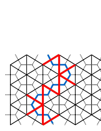
This paper is organized as follows. In section 2 we will recapitulate the TY inequality for SU(2)𝑆𝑈2SU(2) and then prove its generalization to SU(N)𝑆𝑈𝑁SU(N). We will use the two-dimensional SU(N)𝑆𝑈𝑁SU(N) LGT to illustrate our result. In section 3 we will prove a generalization of the inequality to general classical spin systems. We will use the one-dimensional PCM and the two-dimensional Ising models on square and triangular lattices to illustrate the proved inequality. Especially, in section 3.5, we derive a rigorous upper bound of the off-axis correlation length in the triangular Ising model, whose exact expression is still unknown, and conjecture that it is indeed the exact one. In section 3.6 the strong coupling expansion technique is employed to shed light on the implication of our theorem, as well as to test the conjecture. Section 4 is devoted to the conclusion.

2 TY inequality in LGT

2.1 N=2𝑁2N=2

Let us recapitulate the TY inequality for SU(2)𝑆𝑈2SU(2) [1]. ΛΛ\Lambda is a d𝑑d-dimensional hypercubic lattice of length Lμsubscript𝐿𝜇L_{\mu} (μ=1,,d𝜇1𝑑\mu=1,\dots,d) with periodic boundary condition and 𝒱𝒱\mathcal{V}, called “vortex”, is a stacked set of plaquettes winding around the lattice ΛΛ\Lambda in d2𝑑2d-2 periodic directions.555𝒱𝒱\mathcal{V} forms a closed loop when d=3𝑑3d=3 and a closed surface (2-torus) when d=4𝑑4d=4, on the dual lattice. See fig.1. We assume the directions unwrapped by 𝒱𝒱\mathcal{V} to be xμsuperscript𝑥𝜇x^{\mu} and xνsuperscript𝑥𝜈x^{\nu} (μν𝜇𝜈\mu\not=\nu). The ordinary and the “twisted” partition functions are given by

ZΛsubscript𝑍Λ\displaystyle Z_{\Lambda} bdUbexp(β 2pΛTrUp),absentsubscriptproduct𝑏𝑑subscript𝑈𝑏superscript𝛽absentsubscript2absentsubscript𝑝ΛTrsubscript𝑈𝑝\displaystyle\equiv\displaystyle\int\prod_{b}dU_{b}\,\exp\left(\displaystyle\frac{\,\beta\,^{\mathstrut}}{\,2\,_{\mathstrut}}\displaystyle\sum_{p\subset\Lambda}\mathrm{Tr\,}U_{p}\right), (2)
ZΛ()subscriptsuperscript𝑍Λ\displaystyle Z^{(-)}_{\Lambda} bdUbexp(β 2[p𝒱Tr(Up)+pΛ𝒱TrUp]),absentsubscriptproduct𝑏𝑑subscript𝑈𝑏superscript𝛽absentsubscript2absentdelimited-[]subscript𝑝𝒱Trsubscript𝑈𝑝subscript𝑝Λ𝒱Trsubscript𝑈𝑝\displaystyle\equiv\displaystyle\int\prod_{b}dU_{b}\,\exp\left(\displaystyle\frac{\,\beta\,^{\mathstrut}}{\,2\,_{\mathstrut}}\Bigg{[}\displaystyle\sum_{p\subset\mathcal{V}}\mathrm{Tr\,}(-U_{p})+\displaystyle\sum_{p\subset\Lambda\setminus\mathcal{V}}\mathrm{Tr\,}U_{p}\Bigg{]}\right), (3)

where dU𝑑𝑈dU is the normalized Haar measure of SU(2)𝑆𝑈2SU(2) and UpUx,μUx+μ,νUx+ν,μUx,νsubscript𝑈𝑝subscript𝑈𝑥𝜇subscript𝑈𝑥𝜇𝜈subscriptsuperscript𝑈𝑥𝜈𝜇subscriptsuperscript𝑈𝑥𝜈U_{p}\equiv U_{x,\mu}U_{x+\mu,\nu}U^{\dagger}_{x+\nu,\mu}U^{\dagger}_{x,\nu} is a plaquette variable. It is important that local redefinition of variables UU𝑈𝑈U\to-U can move the locations of twisted plaquettes but cannot remove the twist from ΛΛ\Lambda entirely.

Next, consider a rectangle C𝐶C lying in a xμsuperscript𝑥𝜇x^{\mu}-xνsuperscript𝑥𝜈x^{\nu} plane with ACsubscript𝐴𝐶A_{C} the area enclosed by C𝐶C, and let W(C)𝑊𝐶W(C) the Wilson loop in the fundamental representation associated with C𝐶C, namely W(C) 1 2TrbCUb𝑊𝐶superscript1absentsubscript2absentTrsubscriptproduct𝑏𝐶subscript𝑈𝑏\displaystyle W(C)\equiv\displaystyle\frac{\,1\,^{\mathstrut}}{\,2\,_{\mathstrut}}{\mathrm{Tr}\,}\prod_{b\in C}U_{b}. Then the following inequality holds [1, 22]:

Theorem 1.
W(C)2{ 1 2(1ZΛ()ZΛ)}AC/LμLν\langle W(C)\rangle\leq 2\left\{\displaystyle\frac{\,1\,^{\mathstrut}}{\,2\,_{\mathstrut}}\left(1-\displaystyle\frac{\,Z_{\Lambda}^{(-)}\,{}^{\mathstrut}}{\,Z_{\Lambda}\,{}_{\mathstrut}}\right)\right\}^{A_{C}/L_{\mu}L_{\nu}} (4)

where delimited-⟨⟩\langle\dots\rangle is the expectation value w.r.t. the measure of ZΛsubscript𝑍ΛZ_{\Lambda}.

The site-reflection positivity of the Wilson action [23] plays an essential role in the proof. (As is well known, the Wilson action is among those actions for which the link-reflection positivity is also satisfied [24] but it is not a matter of interest here.) Indeed (4) can be proved with any one-plaquette action, since they are site-reflection positive (although not necessarily link-reflection positive, of course).

An important implication of (4) is that the area-law decay of W(C)delimited-⟨⟩𝑊𝐶\langle W(C)\rangle would follow if 1ZΛ()/ZΛeρLμLν1superscriptsubscript𝑍Λsubscript𝑍Λsuperscripte𝜌subscript𝐿𝜇subscript𝐿𝜈1-Z_{\Lambda}^{(-)}/Z_{\Lambda}\approx{\mathrm{e}}^{-\rho L_{\mu}L_{\nu}} for some constant ρ>0𝜌0\rho>0 in the thermodynamic limit666We neglected the entropy factor for simplicity.. This is a famous criterion of confinement originally proposed by ’t Hooft [5] and is also numerically supported [25, 26, 27]. Moreover such a behavior of ZΛ()/ZΛsuperscriptsubscript𝑍Λsubscript𝑍ΛZ_{\Lambda}^{(-)}/Z_{\Lambda} has been verified explicitly by Mu¨nsterM¨unster\rm{M\ddot{u}nster} using the convergent strong-coupling cluster expansion technique [28]. See page 2 for more discussion on this point.

Theorem 1 was utilized in a recent attempt at a rigorous proof of confinement [29] with related discussions [30, 31].

2.2 General N𝑁N

The authors of ref.[1] state without explicit construction that their result is extendable to any other gauge group with nontrivial center. Since the mentioned extension does not seem to be so trivial and, to the author’s best knowledge an explicit formula for general N𝑁N is not found in the literature, we think it valuable to present the extension of (4) from SU(2)𝑆𝑈2SU(2) to SU(N)𝑆𝑈𝑁SU(N) together with its proof.

Let us give a formulation of vortices in SU(N)𝑆𝑈𝑁SU(N) LGT and prove their properties before presenting TY inequality in SU(N)𝑆𝑈𝑁SU(N) LGT. The ordinary and the “twisted” partition functions are respectively given by

ZΛsubscript𝑍Λ\displaystyle Z_{\Lambda} bdUbexp(βNpΛReTrUp),absentsubscriptproduct𝑏𝑑subscript𝑈𝑏superscript𝛽absentsubscript𝑁absentsubscript𝑝ΛReTrsubscript𝑈𝑝\displaystyle\equiv\displaystyle\int\prod_{b}dU_{b}\,\exp\left(\displaystyle\frac{\,\beta\,^{\mathstrut}}{\,N\,_{\mathstrut}}\displaystyle\sum_{p\subset\Lambda}\mathrm{Re\,Tr\,}U_{p}\right), (5)
ZΛ[k]subscriptsuperscript𝑍delimited-[]𝑘Λ\displaystyle Z^{[k]}_{\Lambda} bdUbexp(βN[p𝒱ReTr(zkUp)+pΛ𝒱ReTrUp]),absentsubscriptproduct𝑏𝑑subscript𝑈𝑏superscript𝛽absentsubscript𝑁absentdelimited-[]subscript𝑝𝒱ReTrsuperscript𝑧𝑘subscript𝑈𝑝subscript𝑝Λ𝒱ReTrsubscript𝑈𝑝\displaystyle\equiv\displaystyle\int\prod_{b}dU_{b}\,\exp\left(\displaystyle\frac{\,\beta\,^{\mathstrut}}{\,N\,_{\mathstrut}}\Bigg{[}\displaystyle\sum_{p\subset\mathcal{V}}\mathrm{Re\,Tr\,}(z^{k}U_{p})+\displaystyle\sum_{p\subset\Lambda\setminus\mathcal{V}}\mathrm{Re\,Tr\,}U_{p}\Bigg{]}\right), (6)
zexp(2πiN),k1,2,,N1(modN).formulae-sequence𝑧2𝜋𝑖𝑁𝑘12𝑁1mod𝑁z\equiv\exp\Big{(}\frac{2\pi i}{N}\Big{)},\ \ k\equiv 1,2,...,N-1\,({\rm mod}\ N). (7)

Hereafter delimited-⟨⟩\langle\dots\rangle represents the expectation value with the measure (5). The vortex creation operators {𝒪[k]}superscript𝒪delimited-[]𝑘\{\mathcal{O}^{[k]}\} and the electric flux creation operators {[m]}superscriptdelimited-[]𝑚\{\mathcal{F}^{[m]}\} are defined by

𝒪[k][𝒱]ZΛ[k]ZΛ,\displaystyle\langle\mathcal{O}^{[k]}[\mathcal{V}]\rangle\equiv\displaystyle\frac{\,Z_{\Lambda}^{[k]}\,{}^{\mathstrut}}{\,Z_{\Lambda}\,{}_{\mathstrut}}, (8)
[m][𝒱] 1Nk=0N1zmk𝒪[k][𝒱].delimited-⟨⟩superscriptdelimited-[]𝑚delimited-[]𝒱superscript1absentsubscript𝑁absentsuperscriptsubscript𝑘0𝑁1superscript𝑧𝑚𝑘delimited-⟨⟩superscript𝒪delimited-[]𝑘delimited-[]𝒱\displaystyle\langle\mathcal{F}^{[m]}[\mathcal{V}]\rangle\equiv\displaystyle\frac{\,1\,^{\mathstrut}}{\,N\,_{\mathstrut}}\displaystyle\sum_{k=0}^{N-1}z^{mk}\langle\mathcal{O}^{[k]}[\mathcal{V}]\rangle. (9)

Thus we have 𝒪[k][𝒱]=m=0N1zkm[m][𝒱]delimited-⟨⟩superscript𝒪delimited-[]𝑘delimited-[]𝒱superscriptsubscript𝑚0𝑁1superscript𝑧𝑘𝑚delimited-⟨⟩superscriptdelimited-[]𝑚delimited-[]𝒱\langle\mathcal{O}^{[k]}[\mathcal{V}]\rangle=\displaystyle\sum_{m=0}^{N-1}z^{-km}\langle\mathcal{F}^{[m]}[\mathcal{V}]\rangle. The explicit form of 𝒪𝒪\mathcal{O} is given by

𝒪[k][𝒱]=exp(βNp𝒱[ReTr(zkUp)ReTrUp]).superscript𝒪delimited-[]𝑘delimited-[]𝒱superscript𝛽absentsubscript𝑁absentsubscript𝑝𝒱delimited-[]ReTrsuperscript𝑧𝑘subscript𝑈𝑝ReTrsubscript𝑈𝑝\mathcal{O}^{[k]}[\mathcal{V}]=\exp\Big{(}\displaystyle\frac{\,\beta\,^{\mathstrut}}{\,N\,_{\mathstrut}}\displaystyle\sum_{p\subset\mathcal{V}}[\mathrm{Re\,Tr\,}(z^{k}U_{p})-\mathrm{Re\,Tr\,}U_{p}]\Big{)}. (10)
Lemma 1.

If 𝒱,𝒱,𝒱′′,𝒱superscript𝒱superscript𝒱′′italic-…\mathcal{V},\,\mathcal{V}^{\prime},\,\mathcal{V}^{\prime\prime},\dots are homologous777Plural vortices are called homologous if and only if they wind around the same periodic directions of ΛΛ\Lambda., we have

𝒪[k][𝒱]𝒪[k][𝒱]=𝒪[k+k][𝒱],delimited-⟨⟩superscript𝒪delimited-[]𝑘delimited-[]𝒱superscript𝒪delimited-[]superscript𝑘delimited-[]superscript𝒱delimited-⟨⟩superscript𝒪delimited-[]𝑘superscript𝑘delimited-[]𝒱\displaystyle\langle\mathcal{O}^{[k]}[\mathcal{V}]\mathcal{O}^{[k^{\prime}]}[\mathcal{V}^{\prime}]\rangle=\langle\mathcal{O}^{[k+k^{\prime}]}[\mathcal{V}]\rangle, (11)
m=0N1[m][𝒱]=1,superscriptsubscript𝑚0𝑁1superscriptdelimited-[]𝑚delimited-[]𝒱1\displaystyle\displaystyle\sum_{m=0}^{N-1}\mathcal{F}^{[m]}[\mathcal{V}]=1, (12)
[l][𝒱][m][𝒱]=[l][𝒱]δl,m(N),delimited-⟨⟩superscriptdelimited-[]𝑙delimited-[]𝒱superscriptdelimited-[]𝑚delimited-[]superscript𝒱delimited-⟨⟩superscriptdelimited-[]𝑙delimited-[]𝒱subscriptsuperscript𝛿𝑁𝑙𝑚\displaystyle\langle\mathcal{F}^{[l]}[\mathcal{V}]\mathcal{F}^{[m]}[\mathcal{V}^{\prime}]\rangle=\langle\mathcal{F}^{[l]}[\mathcal{V}]\rangle\,\delta^{(N)}_{l,m}, (13)
[l][𝒱][m][𝒱][n][𝒱′′]=[l][𝒱]δl,m(N)δm,n(N),delimited-⟨⟩superscriptdelimited-[]𝑙delimited-[]𝒱superscriptdelimited-[]𝑚delimited-[]superscript𝒱superscriptdelimited-[]𝑛delimited-[]superscript𝒱′′delimited-⟨⟩superscriptdelimited-[]𝑙delimited-[]𝒱subscriptsuperscript𝛿𝑁𝑙𝑚subscriptsuperscript𝛿𝑁𝑚𝑛\displaystyle\langle\mathcal{F}^{[l]}[\mathcal{V}]\mathcal{F}^{[m]}[\mathcal{V}^{\prime}]\mathcal{F}^{[n]}[\mathcal{V}^{\prime\prime}]\rangle=\langle\mathcal{F}^{[l]}[\mathcal{V}]\rangle\,\delta^{(N)}_{l,m}\delta^{(N)}_{m,n}, (14)
\displaystyle\vdots

where δl,m(N)=1subscriptsuperscript𝛿𝑁𝑙𝑚1\delta^{(N)}_{l,m}=1 if lm𝑙𝑚l\equiv m (mod N𝑁N) and δl,m(N)=0subscriptsuperscript𝛿𝑁𝑙𝑚0\delta^{(N)}_{l,m}=0 otherwise.

Proof.

(11) can be derived by iterating the redefinition of variables UzkU𝑈superscript𝑧superscript𝑘𝑈U\to z^{k^{\prime}}U to bring 𝒱superscript𝒱\mathcal{V}^{\prime} to 𝒱𝒱\mathcal{V}. Relations (12)-(14) follow from (9) and (11). ∎

(12)-(14) imply that {[m]}msubscriptsuperscriptdelimited-[]𝑚𝑚\{\mathcal{F}^{[m]}\}_{m} can be seen as projection operators [5, 11].

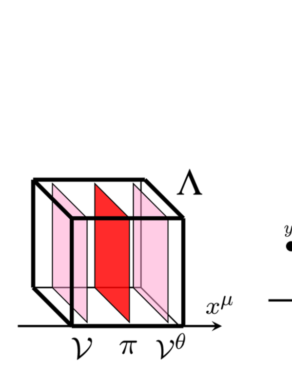
Consider a (d1)𝑑1(d-1)-dimensional hyperplane π𝜋\pi defined by xμ=msuperscript𝑥𝜇𝑚x^{\mu}=m with m𝑚m\in\mathbb{Z} fixed.888 In this paper we never use hyperplanes defined by xμ=m+12superscript𝑥𝜇𝑚12x^{\mu}=m+\frac{1}{2}; that is, we never use link-reflections. Define the reflection operator θ𝜃\theta w.r.t. π𝜋\pi by θ[F({Ub})]=F({Uθ[b]})¯𝜃delimited-[]𝐹subscript𝑈𝑏¯𝐹subscript𝑈𝜃delimited-[]𝑏\theta\big{[}F(\{U_{b}\})\big{]}=\overline{F(\{U_{\theta[b]}\})} where F𝐹F is an arbitrary observable (that is, a map from configurations on ΛΛ\Lambda to \mathbb{C}). The reflection θ[b]𝜃delimited-[]𝑏\theta[b] of a link b𝑏b is also defined by the same notation where locations of b𝑏b and θ[b]𝜃delimited-[]𝑏\theta[b], are defined to be symmetrical about π𝜋\pi.

Lemma 2.

With 𝒱θθ[𝒱]superscript𝒱𝜃𝜃delimited-[]𝒱\mathcal{V}^{\theta}\equiv\theta[\mathcal{V}] we have

θ[𝒪[k][𝒱]]=𝒪[k][𝒱θ],𝜃delimited-[]superscript𝒪delimited-[]𝑘delimited-[]𝒱superscript𝒪delimited-[]𝑘delimited-[]superscript𝒱𝜃\displaystyle\theta\Big{[}\mathcal{O}^{[k]}[\mathcal{V}]\Big{]}=\mathcal{O}^{[-k]}[\mathcal{V}^{\theta}], (15)
θ[[m][𝒱]]=[m][𝒱θ],𝜃delimited-[]superscriptdelimited-[]𝑚delimited-[]𝒱superscriptdelimited-[]𝑚delimited-[]superscript𝒱𝜃\displaystyle\theta\Big{[}\mathcal{F}^{[m]}[\mathcal{V}]\Big{]}=\mathcal{F}^{[m]}[\mathcal{V}^{\theta}], (16)
0𝒪[k][𝒱]1,0delimited-⟨⟩superscript𝒪delimited-[]𝑘delimited-[]𝒱1\displaystyle 0\leq\langle\mathcal{O}^{[k]}[\mathcal{V}]\rangle\leq 1, (17)
0[m][𝒱]1.0delimited-⟨⟩superscriptdelimited-[]𝑚delimited-[]𝒱1\displaystyle 0\leq\langle\mathcal{F}^{[m]}[\mathcal{V}]\rangle\leq 1. (18)
Proof.

(15) is obvious from the fact that the orientation of plaquettes are reversed by reflection. (15) yields

θ[[m][𝒱]]𝜃delimited-[]superscriptdelimited-[]𝑚delimited-[]𝒱\displaystyle\theta\Big{[}\mathcal{F}^{[m]}[\mathcal{V}]\Big{]} =θ[ 1Nk=0N1zmk𝒪[k][𝒱]]absent𝜃delimited-[]superscript1absentsubscript𝑁absentsuperscriptsubscript𝑘0𝑁1superscript𝑧𝑚𝑘superscript𝒪delimited-[]𝑘delimited-[]𝒱\displaystyle=\theta\Big{[}\displaystyle\frac{\,1\,^{\mathstrut}}{\,N\,_{\mathstrut}}\displaystyle\sum_{k=0}^{N-1}z^{mk}\mathcal{O}^{[k]}[\mathcal{V}]\Big{]} (19)
= 1Nk=0N1zmk𝒪[k][𝒱θ]absentsuperscript1absentsubscript𝑁absentsuperscriptsubscript𝑘0𝑁1superscript𝑧𝑚𝑘superscript𝒪delimited-[]𝑘delimited-[]superscript𝒱𝜃\displaystyle=\displaystyle\frac{\,1\,^{\mathstrut}}{\,N\,_{\mathstrut}}\displaystyle\sum_{k=0}^{N-1}z^{-mk}\mathcal{O}^{[-k]}[\mathcal{V}^{\theta}] (20)
=[m][𝒱θ]absentsuperscriptdelimited-[]𝑚delimited-[]superscript𝒱𝜃\displaystyle=\mathcal{F}^{[m]}[\mathcal{V}^{\theta}] (21)

which proves (16). Next, using the Schwarz inequality |F|FθF1/2delimited-⟨⟩𝐹superscriptdelimited-⟨⟩𝐹𝜃𝐹12|\langle F\rangle|\leq\langle F\theta F\rangle^{1/2} and (11), (15) we find

𝒪[k][𝒱]delimited-⟨⟩superscript𝒪delimited-[]𝑘delimited-[]𝒱\displaystyle\langle\mathcal{O}^{[k]}[\mathcal{V}]\rangle 𝒪[k][𝒱]θ[𝒪[k][𝒱]]1/2absentsuperscriptdelimited-⟨⟩superscript𝒪delimited-[]𝑘delimited-[]𝒱𝜃delimited-[]superscript𝒪delimited-[]𝑘delimited-[]𝒱12\displaystyle\leq\langle\mathcal{O}^{[k]}[\mathcal{V}]\theta\Big{[}\mathcal{O}^{[k]}[\mathcal{V}]\Big{]}\rangle^{1/2} (22)
=𝒪[k][𝒱]𝒪[k][𝒱θ]1/2=1.absentsuperscriptdelimited-⟨⟩superscript𝒪delimited-[]𝑘delimited-[]𝒱superscript𝒪delimited-[]𝑘delimited-[]superscript𝒱𝜃121\displaystyle=\langle\mathcal{O}^{[k]}[\mathcal{V}]\mathcal{O}^{[-k]}[\mathcal{V}^{\theta}]\rangle^{1/2}=1. (23)

which proves the second inequality in (17) while the first one is trivial. Since 𝒱𝒱\mathcal{V} and 𝒱θsuperscript𝒱𝜃\mathcal{V}^{\theta} are homologous we can apply (13) to obtain

[m][𝒱]delimited-⟨⟩superscriptdelimited-[]𝑚delimited-[]𝒱\displaystyle\langle\mathcal{F}^{[m]}[\mathcal{V}]\rangle =[m][𝒱][m][𝒱θ]absentdelimited-⟨⟩superscriptdelimited-[]𝑚delimited-[]𝒱superscriptdelimited-[]𝑚delimited-[]superscript𝒱𝜃\displaystyle=\langle\mathcal{F}^{[m]}[\mathcal{V}]\mathcal{F}^{[m]}[\mathcal{V}^{\theta}]\rangle (24)
=[m][𝒱]θ[[m][𝒱]]0.absentdelimited-⟨⟩superscriptdelimited-[]𝑚delimited-[]𝒱𝜃delimited-[]superscriptdelimited-[]𝑚delimited-[]𝒱0\displaystyle=\langle\mathcal{F}^{[m]}[\mathcal{V}]\theta\Big{[}\mathcal{F}^{[m]}[\mathcal{V}]\Big{]}\rangle\geq 0. (25)

(25) and (12) prove (18). (These simple proofs of (17) and (18) seem to be new.) ∎

The vortex free energy Fv[k]superscriptsubscript𝐹𝑣delimited-[]𝑘F_{v}^{[k]} and the electric flux free energy Fel[m]superscriptsubscript𝐹𝑒𝑙delimited-[]𝑚F_{el}^{[m]} are defined by eFv[k]𝒪[k][𝒱]superscriptesuperscriptsubscript𝐹𝑣delimited-[]𝑘delimited-⟨⟩superscript𝒪delimited-[]𝑘delimited-[]𝒱{\mathrm{e}}^{-F_{v}^{[k]}}\equiv\langle\mathcal{O}^{[k]}[\mathcal{V}]\rangle and eFel[m][m][𝒱]superscriptesuperscriptsubscript𝐹𝑒𝑙delimited-[]𝑚delimited-⟨⟩superscriptdelimited-[]𝑚delimited-[]𝒱{\mathrm{e}}^{-F_{el}^{[m]}}\equiv\langle\mathcal{F}^{[m]}[\mathcal{V}]\rangle, respectively.

Let N(R){0,1,,N1}𝑁𝑅01𝑁1N(R)\in\{0,1,\dots,N-1\} denote the N𝑁N-ality of an irreducible representation R𝑅R999N𝑁N-ality is the number (mod N𝑁N) of boxes in the Young tableau of R𝑅R. of SU(N)𝑆𝑈𝑁SU(N) whose dimension is dRsubscript𝑑𝑅d_{R}. Take a rectangle C𝐶C lying in a xμsuperscript𝑥𝜇x^{\mu}-xνsuperscript𝑥𝜈x^{\nu} plane and let ACsubscript𝐴𝐶A_{C} the area enclosed by C𝐶C. For the normalized Wilson loop in the representation R𝑅R, WR(C) 1dRχR(bCUb)W_{R}(C)\equiv\displaystyle\frac{\,1\,^{\mathstrut}}{\,d_{R}\,{}_{\mathstrut}}\chi_{R}\Big{(}\prod_{b\in C}U_{b}\Big{)}, we have

Theorem 2 (TY inequality for SU(N)𝑆𝑈𝑁SU(N) LGT).
|WR(C)|[N(R)][𝒱]AC/LμLν+{1[0][𝒱]}AC/LμLν.delimited-⟨⟩subscript𝑊𝑅𝐶superscriptdelimited-⟨⟩superscriptdelimited-[]𝑁𝑅delimited-[]𝒱subscript𝐴𝐶subscript𝐿𝜇subscript𝐿𝜈superscript1delimited-⟨⟩superscriptdelimited-[]0delimited-[]𝒱subscript𝐴𝐶subscript𝐿𝜇subscript𝐿𝜈|\langle W_{R}(C)\rangle|\leq\langle\mathcal{F}^{[N(R)]}[\mathcal{V}]\rangle^{A_{C}/L_{\mu}L_{\nu}}+\left\{1-\langle\mathcal{F}^{[0]}[\mathcal{V}]\rangle\right\}^{A_{C}/L_{\mu}L_{\nu}}. (26)

In addition, if N(R)0𝑁𝑅0N(R)\not=0 we have

|WR(C)|delimited-⟨⟩subscript𝑊𝑅𝐶\displaystyle|\langle W_{R}(C)\rangle| 2{1[0][𝒱]}AC/LμLνabsent2superscript1delimited-⟨⟩superscriptdelimited-[]0delimited-[]𝒱subscript𝐴𝐶subscript𝐿𝜇subscript𝐿𝜈\displaystyle\leq 2\left\{1-\langle\mathcal{F}^{[0]}[\mathcal{V}]\rangle\right\}^{A_{C}/L_{\mu}L_{\nu}} (27)
=2{1 1Nk=0N1𝒪[k][𝒱]}AC/LμLν.absent2superscript1superscript1absentsubscript𝑁absentsuperscriptsubscript𝑘0𝑁1delimited-⟨⟩superscript𝒪delimited-[]𝑘delimited-[]𝒱subscript𝐴𝐶subscript𝐿𝜇subscript𝐿𝜈\displaystyle=2\left\{1-\displaystyle\frac{\,1\,^{\mathstrut}}{\,N\,_{\mathstrut}}\displaystyle\sum_{k=0}^{N-1}\langle\mathcal{O}^{[k]}[\mathcal{V}]\rangle\right\}^{A_{C}/L_{\mu}L_{\nu}}. (28)
Proof.

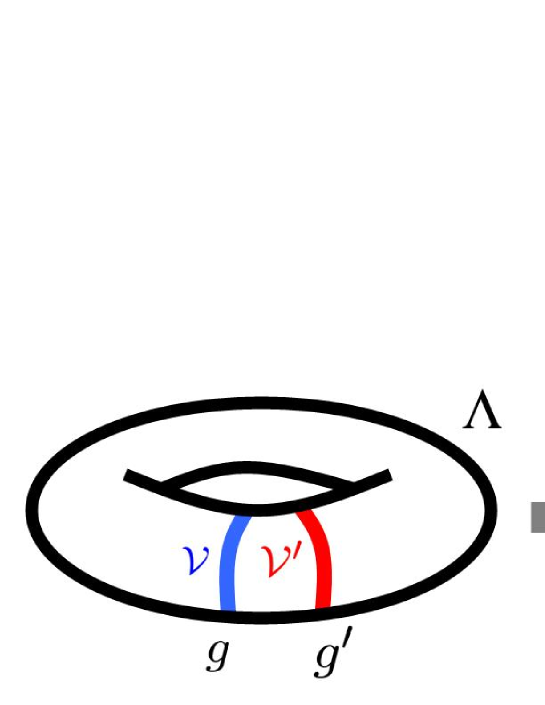
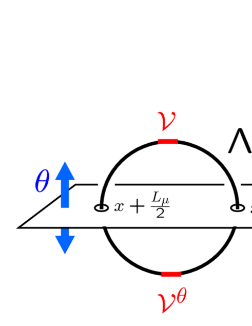
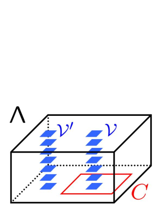
Although the argument below parallels that of ref.[22] for SU(2)𝑆𝑈2SU(2), we describe the proof in full detail for readers’ convenience. Suppose 𝒱,𝒱𝒱superscript𝒱\mathcal{V},\,\mathcal{V}^{\prime} are stacked set of plaquettes wrapping around d2𝑑2d-2 periodic directions of ΛΛ\Lambda and 𝒱𝒱\mathcal{V} is linking once with C𝐶C while 𝒱superscript𝒱\mathcal{V}^{\prime} is not. (See fig.1 for a 3-dimensional illustration of the setting.)
Refer to caption
Figure 1: Locations of 𝒱,𝒱𝒱superscript𝒱\mathcal{V},\,\mathcal{V}^{\prime} and C𝐶C.

Let us rewrite the expectation value of WR(C) 1dRχR(bCUb)W_{R}(C)\equiv\displaystyle\frac{\,1\,^{\mathstrut}}{\,d_{R}\,{}_{\mathstrut}}\chi_{R}\Big{(}\displaystyle\prod_{b\in C}U_{b}\Big{)} as follows:

WR(C)delimited-⟨⟩subscript𝑊𝑅𝐶\displaystyle\langle W_{R}(C)\rangle =(1[0][𝒱])WR(C)+[0][𝒱]WR(C)absentdelimited-⟨⟩1superscriptdelimited-[]0delimited-[]𝒱subscript𝑊𝑅𝐶delimited-⟨⟩superscriptdelimited-[]0delimited-[]𝒱subscript𝑊𝑅𝐶\displaystyle=\langle(1-\mathcal{F}^{[0]}[\mathcal{V}])W_{R}(C)\rangle+\langle\mathcal{F}^{[0]}[\mathcal{V}]W_{R}(C)\rangle (29)
=(1[0][𝒱])WR(C)+ 1Nk=0N1𝒪[k][𝒱]WR(C).absentdelimited-⟨⟩1superscriptdelimited-[]0delimited-[]𝒱subscript𝑊𝑅𝐶superscript1absentsubscript𝑁absentsuperscriptsubscript𝑘0𝑁1delimited-⟨⟩superscript𝒪delimited-[]𝑘delimited-[]𝒱subscript𝑊𝑅𝐶\displaystyle=\langle(1-\mathcal{F}^{[0]}[\mathcal{V}])W_{R}(C)\rangle+\displaystyle\frac{\,1\,^{\mathstrut}}{\,N\,_{\mathstrut}}\displaystyle\sum_{k=0}^{N-1}\langle\mathcal{O}^{[k]}[\mathcal{V}]W_{R}(C)\rangle. (30)

The presence of the second term is not desirable from the viewpoint of obtaining a meaningful upper bound of WR(C)delimited-⟨⟩subscript𝑊𝑅𝐶\langle W_{R}(C)\rangle, so let us perform redefinitions of variables UzkU𝑈superscript𝑧𝑘𝑈U\to z^{k}U to bring 𝒱𝒱\mathcal{V} to 𝒱superscript𝒱\mathcal{V}^{\prime}, which causes the change

𝒪[k][𝒱]WR(C)z±N(R)k𝒪[k][𝒱]WR(C).delimited-⟨⟩superscript𝒪delimited-[]𝑘delimited-[]𝒱subscript𝑊𝑅𝐶superscript𝑧plus-or-minus𝑁𝑅𝑘delimited-⟨⟩superscript𝒪delimited-[]𝑘delimited-[]superscript𝒱subscript𝑊𝑅𝐶\langle\mathcal{O}^{[k]}[\mathcal{V}]W_{R}(C)\rangle\to z^{\pm N(R)k}\langle\mathcal{O}^{[k]}[\mathcal{V}^{\prime}]W_{R}(C)\rangle. (31)

This is because in the course of bringing 𝒱𝒱\mathcal{V} to 𝒱superscript𝒱\mathcal{V}^{\prime} we must change one of the link variables on C𝐶C. (The sign of exponent depends on the orientation of C𝐶C.) Thus (30) becomes

WR(C)delimited-⟨⟩subscript𝑊𝑅𝐶\displaystyle\langle W_{R}(C)\rangle =(1[0][𝒱])WR(C)+ 1Nk=0N1z±N(R)k𝒪[k][𝒱]WR(C)absentdelimited-⟨⟩1superscriptdelimited-[]0delimited-[]𝒱subscript𝑊𝑅𝐶superscript1absentsubscript𝑁absentsuperscriptsubscript𝑘0𝑁1superscript𝑧plus-or-minus𝑁𝑅𝑘delimited-⟨⟩superscript𝒪delimited-[]𝑘delimited-[]superscript𝒱subscript𝑊𝑅𝐶\displaystyle=\langle(1-\mathcal{F}^{[0]}[\mathcal{V}])W_{R}(C)\rangle+\displaystyle\frac{\,1\,^{\mathstrut}}{\,N\,_{\mathstrut}}\displaystyle\sum_{k=0}^{N-1}z^{\pm N(R)k}\langle\mathcal{O}^{[k]}[\mathcal{V}^{\prime}]W_{R}(C)\rangle (32)
=(1[0][𝒱])WR(C)+[±N(R)][𝒱]WR(C).absentdelimited-⟨⟩1superscriptdelimited-[]0delimited-[]𝒱subscript𝑊𝑅𝐶delimited-⟨⟩superscriptdelimited-[]plus-or-minus𝑁𝑅delimited-[]superscript𝒱subscript𝑊𝑅𝐶\displaystyle=\langle(1-\mathcal{F}^{[0]}[\mathcal{V}])W_{R}(C)\rangle+\langle\mathcal{F}^{[\pm N(R)]}[\mathcal{V}^{\prime}]W_{R}(C)\rangle. (33)
Refer to caption
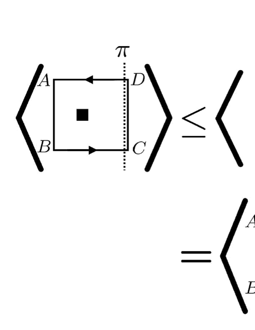
Figure 2: The Schwarz inequality enables us to double the size of the rectangle. This figure is essentially borrowed from ref.[22].

Our next step is expressed in fig.2 schematically in which a black square represents the operator (1[0][𝒱])1superscriptdelimited-[]0delimited-[]𝒱(1-\mathcal{F}^{[0]}[\mathcal{V}]). Labeling four vertices as A,B,C,D𝐴𝐵𝐶𝐷A,B,C,D, setting the hyperplane π𝜋\pi so that it is perpendicular to the rectangle and contains the edge CD𝐶𝐷CD, and applying the Schwarz inequality |FθG|FθF1/2GθG1/2delimited-⟨⟩𝐹𝜃𝐺superscriptdelimited-⟨⟩𝐹𝜃𝐹12superscriptdelimited-⟨⟩𝐺𝜃𝐺12|\langle F\theta G\rangle|\leq\langle F\theta F\rangle^{1/2}\langle G\theta G\rangle^{1/2} we obtain

|(1[0][𝒱])WR|DA+AB+BC+CD|\displaystyle\big{|}\langle(1-\mathcal{F}^{[0]}[\mathcal{V}])W_{R}\big{|}_{DA+AB+BC+CD}\rangle\big{|} (34)
=\displaystyle=\  1dR|(1[0][𝒱])χR|DA+AB+BC+CD|\displaystyle\displaystyle\frac{\,1\,^{\mathstrut}}{\,d_{R}\,{}_{\mathstrut}}\big{|}\langle(1-\mathcal{F}^{[0]}[\mathcal{V}])\chi_{R}\big{|}_{DA+AB+BC+CD}\rangle\big{|} (35)
=\displaystyle=\  1dR|α,β(1[0][𝒱]){χR|DA+AB+BC}αβ{χR|CD}βα|\displaystyle\displaystyle\frac{\,1\,^{\mathstrut}}{\,d_{R}\,{}_{\mathstrut}}\Big{|}\displaystyle\sum_{\alpha,\beta}\big{\langle}(1-\mathcal{F}^{[0]}[\mathcal{V}])\{\chi_{R}\big{|}_{DA+AB+BC}\}_{\alpha\beta}\{\chi_{R}\big{|}_{CD}\}_{\beta\alpha}\big{\rangle}\Big{|} (36)
\displaystyle\leq\  1dRα,β(1[0][𝒱])(1[0][𝒱θ]){χR|DA+AB+BC}αβ{χR|DAθ+AθBθ+BθC}αβ¯1/2\displaystyle\displaystyle\frac{\,1\,^{\mathstrut}}{\,d_{R}\,{}_{\mathstrut}}\displaystyle\sum_{\alpha,\beta}\Big{\langle}(1-\mathcal{F}^{[0]}[\mathcal{V}])(1-\mathcal{F}^{[0]}[\mathcal{V}^{\theta}])\{\chi_{R}\big{|}_{DA+AB+BC}\}_{\alpha\beta}\overline{\{\chi_{R}\big{|}_{DA^{\theta}+A^{\theta}B^{\theta}+B^{\theta}C}\}_{\alpha\beta}}\Big{\rangle}^{1/2}
×{χR|CD}βα{χR|CD}βα¯1/2absentsuperscriptdelimited-⟨⟩subscriptevaluated-atsubscript𝜒𝑅𝐶𝐷𝛽𝛼¯subscriptevaluated-atsubscript𝜒𝑅𝐶𝐷𝛽𝛼12\displaystyle\hskip 100.0pt\times\Big{\langle}\{\chi_{R}\big{|}_{CD}\}_{\beta\alpha}\overline{\{\chi_{R}\big{|}_{CD}\}_{\beta\alpha}}\Big{\rangle}^{1/2} (37)
\displaystyle\leq\  1dR(1[0][𝒱])α,β{χR|DA+AB+BC}αβ{χR|DAθ+AθBθ+BθC}αβ¯1/2×dR\displaystyle\displaystyle\frac{\,1\,^{\mathstrut}}{\,d_{R}\,{}_{\mathstrut}}\Big{\langle}(1-\mathcal{F}^{[0]}[\mathcal{V}])\displaystyle\sum_{\alpha,\beta}\{\chi_{R}\big{|}_{DA+AB+BC}\}_{\alpha\beta}\overline{\{\chi_{R}\big{|}_{DA^{\theta}+A^{\theta}B^{\theta}+B^{\theta}C}\}_{\alpha\beta}}\Big{\rangle}^{1/2}\times\sqrt{d_{R}} (38)
=\displaystyle=\ (1[0][𝒱])WR|AB+BBθ+BθAθ+AθA1/2.superscriptdelimited-⟨⟩evaluated-at1superscriptdelimited-[]0delimited-[]𝒱subscript𝑊𝑅𝐴𝐵𝐵superscript𝐵𝜃superscript𝐵𝜃superscript𝐴𝜃superscript𝐴𝜃𝐴12\displaystyle\langle(1-\mathcal{F}^{[0]}[\mathcal{V}])W_{R}\big{|}_{AB+BB^{\theta}+B^{\theta}A^{\theta}+A^{\theta}A}\rangle^{1/2}. (39)

In going from (37) to (38) we used (13). The length of the rectangle doubled.

Let lμ×lνsubscript𝑙𝜇subscript𝑙𝜈l_{\mu}\times l_{\nu} the size of the original rectangle and assume that Lμ=2plμsubscript𝐿𝜇superscript2𝑝subscript𝑙𝜇L_{\mu}=2^{p}l_{\mu} and Lν=2qlνsubscript𝐿𝜈superscript2𝑞subscript𝑙𝜈L_{\nu}=2^{q}l_{\nu} for some p,q𝐍𝑝𝑞𝐍p,q\in\mathbf{N}101010This condition was also present in the original TY inequality [1]. It is not a severe restriction, however, as long as we believe the asymptotic behavior of observables to be independent of the way we take Lμ,Lνsubscript𝐿𝜇subscript𝐿𝜈L_{\mu},\,L_{\nu} to infinity.. Repeating the operation above for sufficiently many times in both xμsuperscript𝑥𝜇x^{\mu}- and xνsuperscript𝑥𝜈x^{\nu}- directions, due to the periodic boundary conditions the rectangle finally vanishes away, yielding

(1[0][𝒱])WR(C)delimited-⟨⟩1superscriptdelimited-[]0delimited-[]𝒱subscript𝑊𝑅𝐶\displaystyle\langle(1-\mathcal{F}^{[0]}[\mathcal{V}])W_{R}(C)\rangle {1[0][𝒱]}1/2p+qabsentsuperscript1delimited-⟨⟩superscriptdelimited-[]0delimited-[]𝒱1superscript2𝑝𝑞\displaystyle\leq\left\{1-\langle\mathcal{F}^{[0]}[\mathcal{V}]\rangle\right\}^{1/2^{p+q}} (40)
={1[0][𝒱]}lμlν/LμLν={1[0][𝒱]}AC/LμLν.absentsuperscript1delimited-⟨⟩superscriptdelimited-[]0delimited-[]𝒱subscript𝑙𝜇subscript𝑙𝜈subscript𝐿𝜇subscript𝐿𝜈superscript1delimited-⟨⟩superscriptdelimited-[]0delimited-[]𝒱subscript𝐴𝐶subscript𝐿𝜇subscript𝐿𝜈\displaystyle=\left\{1-\langle\mathcal{F}^{[0]}[\mathcal{V}]\rangle\right\}^{l_{\mu}l_{\nu}/L_{\mu}L_{\nu}}=\left\{1-\langle\mathcal{F}^{[0]}[\mathcal{V}]\rangle\right\}^{A_{C}/L_{\mu}L_{\nu}}. (41)

[±N(R)][𝒱]WR(C)[±N(R)][𝒱]AC/LμLνdelimited-⟨⟩superscriptdelimited-[]plus-or-minus𝑁𝑅delimited-[]superscript𝒱subscript𝑊𝑅𝐶superscriptdelimited-⟨⟩superscriptdelimited-[]plus-or-minus𝑁𝑅delimited-[]superscript𝒱subscript𝐴𝐶subscript𝐿𝜇subscript𝐿𝜈\langle\mathcal{F}^{[\pm N(R)]}[\mathcal{V}^{\prime}]W_{R}(C)\rangle\leq\langle\mathcal{F}^{[\pm N(R)]}[\mathcal{V}^{\prime}]\rangle^{A_{C}/L_{\mu}L_{\nu}} can be shown in a similar way, hence (26) is proved.

(27) is a consequence of (26) and [N(R)][𝒱]1[0][𝒱]delimited-⟨⟩superscriptdelimited-[]𝑁𝑅delimited-[]𝒱1delimited-⟨⟩superscriptdelimited-[]0delimited-[]𝒱\langle\mathcal{F}^{[N(R)]}[\mathcal{V}]\rangle\leq 1-\langle\mathcal{F}^{[0]}[\mathcal{V}]\rangle. ∎

The message of (28) is that the exponential decay of the vortex free energy, i.e. 𝒪[k][𝒱]eFv[k]=1O(eρLμLν)delimited-⟨⟩superscript𝒪delimited-[]𝑘delimited-[]𝒱superscriptesuperscriptsubscript𝐹𝑣delimited-[]𝑘1𝑂superscripte𝜌subscript𝐿𝜇subscript𝐿𝜈\langle\mathcal{O}^{[k]}[\mathcal{V}]\rangle\equiv{\mathrm{e}}^{-F_{v}^{[k]}}=1-O({\mathrm{e}}^{-\rho L_{\mu}L_{\nu}}) for every k𝑘k, is a sufficient condition for the area law of the Wilson loop to hold. The area law does not hold, or is at least difficult to prove, if not all of the 𝒪delimited-⟨⟩𝒪\langle\mathcal{O}\rangle’s converge to 1.

Several comments are in order. Firstly, suppose that the action in (2) is in the adjoint representation. Then 𝒪[k][𝒱]=1delimited-⟨⟩superscript𝒪delimited-[]𝑘delimited-[]𝒱1\langle\mathcal{O}^{[k]}[\mathcal{V}]\rangle=1 follows for any k𝑘k, hence making WR(C)delimited-⟨⟩subscript𝑊𝑅𝐶\langle W_{R}(C)\rangle with N(R)0𝑁𝑅0N(R)\not=0 vanish identically for arbitrary finite volume (see (28)). This is to be anticipated; since the adjoint Wilson action is invariant under the local transformation UzU𝑈𝑧𝑈U\to zU (zZN)𝑧subscript𝑍𝑁(z\in Z_{N}), which cannot break spontaneously according to the Elitzur’s theorem, and since WR(C)subscript𝑊𝑅𝐶W_{R}(C) with N(R)0𝑁𝑅0N(R)\not=0 transforms nontrivially under this transformation, its expectation value must vanish.

Secondly, there are a lot more varieties of inequalities available other than (26). Assume N=6𝑁6N=6 for instance. From (13) we have ([1][𝒱]+[2][𝒱])([1][𝒱]+[2][𝒱])=[1][𝒱]+[2][𝒱]delimited-⟨⟩superscriptdelimited-[]1delimited-[]𝒱superscriptdelimited-[]2delimited-[]𝒱superscriptdelimited-[]1delimited-[]superscript𝒱superscriptdelimited-[]2delimited-[]superscript𝒱delimited-⟨⟩superscriptdelimited-[]1delimited-[]𝒱superscriptdelimited-[]2delimited-[]𝒱\big{\langle}(\mathcal{F}^{[1]}[\mathcal{V}]+\mathcal{F}^{[2]}[\mathcal{V}])(\mathcal{F}^{[1]}[\mathcal{V}^{\prime}]+\mathcal{F}^{[2]}[\mathcal{V}^{\prime}])\big{\rangle}=\langle\mathcal{F}^{[1]}[\mathcal{V}]+\mathcal{F}^{[2]}[\mathcal{V}]\rangle and ([3][𝒱]+[4][𝒱]+[5][𝒱])([3][𝒱]+[4][𝒱]+[5][𝒱])=[3][𝒱]+[4][𝒱]+[5][𝒱]delimited-⟨⟩superscriptdelimited-[]3delimited-[]𝒱superscriptdelimited-[]4delimited-[]𝒱superscriptdelimited-[]5delimited-[]𝒱superscriptdelimited-[]3delimited-[]superscript𝒱superscriptdelimited-[]4delimited-[]superscript𝒱superscriptdelimited-[]5delimited-[]superscript𝒱delimited-⟨⟩superscriptdelimited-[]3delimited-[]𝒱superscriptdelimited-[]4delimited-[]𝒱superscriptdelimited-[]5delimited-[]𝒱\big{\langle}(\mathcal{F}^{[3]}[\mathcal{V}]+\mathcal{F}^{[4]}[\mathcal{V}]+\mathcal{F}^{[5]}[\mathcal{V}])(\mathcal{F}^{[3]}[\mathcal{V}^{\prime}]+\mathcal{F}^{[4]}[\mathcal{V}^{\prime}]+\mathcal{F}^{[5]}[\mathcal{V}^{\prime}])\big{\rangle}=\langle\mathcal{F}^{[3]}[\mathcal{V}]+\mathcal{F}^{[4]}[\mathcal{V}]+\mathcal{F}^{[5]}[\mathcal{V}]\rangle, hence by modifying the above proof one can straightforwardly show

|WR(C)|[N(R)]AC/LμLν+{[1]+[2]}AC/LμLν+{[3]+[4]+[5]}AC/LμLν.delimited-⟨⟩subscript𝑊𝑅𝐶superscriptdelimited-⟨⟩superscriptdelimited-[]𝑁𝑅subscript𝐴𝐶subscript𝐿𝜇subscript𝐿𝜈superscriptdelimited-⟨⟩superscriptdelimited-[]1superscriptdelimited-[]2subscript𝐴𝐶subscript𝐿𝜇subscript𝐿𝜈superscriptdelimited-⟨⟩superscriptdelimited-[]3superscriptdelimited-[]4superscriptdelimited-[]5subscript𝐴𝐶subscript𝐿𝜇subscript𝐿𝜈|\langle W_{R}(C)\rangle|\leq\langle\mathcal{F}^{[N(R)]}\rangle^{A_{C}/L_{\mu}L_{\nu}}+\left\{\langle\mathcal{F}^{[1]}+\mathcal{F}^{[2]}\rangle\right\}^{A_{C}/L_{\mu}L_{\nu}}+\left\{\langle\mathcal{F}^{[3]}+\mathcal{F}^{[4]}+\mathcal{F}^{[5]}\rangle\right\}^{A_{C}/L_{\mu}L_{\nu}}. (42)

However (42) and all of its cousins are weaker than (26) with N=6𝑁6N=6, which can be understood by the elementary inequality (ixi)α<i(xi)αsuperscriptsubscript𝑖subscript𝑥𝑖𝛼subscript𝑖superscriptsubscript𝑥𝑖𝛼(\sum_{i}x_{i})^{\alpha}<\sum_{i}(x_{i})^{\alpha} for 0<α<10𝛼10<\alpha<1 and 0<xi0subscript𝑥𝑖0<x_{i}.

Note that one cannot derive the area law from (26) when N(R)=0𝑁𝑅0N(R)=0, as can be seen from

[r.h.s.of(26)][0][𝒱]AC/LμLν( 1N)AC/LμLν1asLμ,Lν.\Big{[}{\rm{r.h.s.}}\ {\rm{of}}\ (\ref{N})\Big{]}\geq\langle\mathcal{F}^{[0]}[\mathcal{V}]\rangle^{A_{C}/L_{\mu}L_{\nu}}\geq\Big{(}\displaystyle\frac{\,1\,^{\mathstrut}}{\,N\,_{\mathstrut}}\Big{)}^{A_{C}/L_{\mu}L_{\nu}}\ \ \to 1\ \ {\rm{as}}\ \ L_{\mu},\,L_{\nu}\to\infty. (43)

The above implies that the “gluons” of SU(N)𝑆𝑈𝑁SU(N) can screen particles of zero N𝑁N-ality.

Thirdly, theorem 2 is correct even after a matter field whose N𝑁N-ality is zero is introduced into the theory, since the matter-gauge coupling Φx+μ^Dr[Ux,μ]ΦxsubscriptsuperscriptΦ𝑥^𝜇subscript𝐷𝑟delimited-[]subscript𝑈𝑥𝜇subscriptΦ𝑥\Phi^{\dagger}_{x+\hat{\mu}}D_{r}[U_{x,\mu}]\Phi_{x} preserves reflection positivity and is insensitive to the change of variables UzU𝑈𝑧𝑈U\to zU.

Finally we remark on the utility of strong-coupling cluster expansion techniques. (Similar discussion will be presented in section 3.6.) As already mentioned, the exponential suppression of vortex free energy log𝒪[𝒱]eρLμLν𝒪delimited-[]𝒱superscripte𝜌subscript𝐿𝜇subscript𝐿𝜈-\log\langle\mathcal{O}[\mathcal{V}]\rangle\approx{\mathrm{e}}^{-\rho L_{\mu}L_{\nu}} has been verified by Mu¨nsterM¨unster\rm{M\ddot{u}nster} [28] for SU(2)𝑆𝑈2SU(2) LGT and for sufficiently strong coupling. Especially he showed to all orders of strong-coupling expansion that the constant ρ𝜌\rho appearing in the vortex free energy (’t Hooft’s string tension) is equal to the conventional Wilson’s string tension. His proof hinges on the observation that both the calculation of Wilson loop expectation value and that of vortex free energy reduce, at sufficiently strong coupling, to the problem of fluctuating random surfaces. It is understood without difficulty that the methods he employed can be readily used for SU(N)𝑆𝑈𝑁SU(N) LGT to show log𝒪[k][𝒱]eρLμLνsuperscript𝒪delimited-[]𝑘delimited-[]𝒱superscripte𝜌subscript𝐿𝜇subscript𝐿𝜈-\log\langle\mathcal{O}^{[k]}[\mathcal{V}]\rangle\approx{\mathrm{e}}^{-\rho L_{\mu}L_{\nu}} for every k0𝑘0k\not=0 (hence proving the area law). This time ρ𝜌\rho is equal to the fundamental string tension (since the gauge action (5) is in the fundamental representation).
                        *                        *                        *                        *

Let us then turn to LGT with matter field of non-zero N𝑁N-ality; the relations (11)-(14) are no longer valid. If the matter field has N𝑁N-ality m𝑚m and the greatest common divisor of N𝑁N and m𝑚m is s𝑠s , the subgroup ZsZNsubscript𝑍𝑠subscript𝑍𝑁Z_{s}\subset Z_{N} is a symmetry of the theory. It is thus straightforward to prove the following

Theorem 3.

If N(R)0not-equivalent-to𝑁𝑅0N(R)\not\equiv 0 (mod s𝑠s), we have

|WR(C)|2{1f[0][𝒱]}AC/LμLν=2{1 1sk=0s1ZΛ[kN/s]ZΛ}AC/LμLν.|\langle W_{R}(C)\rangle|\leq 2\left\{1-\langle f^{[0]}[\mathcal{V}]\rangle\right\}^{A_{C}/L_{\mu}L_{\nu}}=2\left\{1-\displaystyle\frac{\,1\,^{\mathstrut}}{\,s\,_{\mathstrut}}\displaystyle\sum_{k=0}^{s-1}\displaystyle\frac{\,Z_{\Lambda}^{[kN/s]}\,{}^{\mathstrut}}{\,Z_{\Lambda}\,{}_{\mathstrut}}\right\}^{A_{C}/L_{\mu}L_{\nu}}. (44)

Although the development so far has been for SU(N)𝑆𝑈𝑁SU(N) LGT, the inequalities evidently apply to U(N)𝑈𝑁U(N) LGT since the center of U(N)𝑈𝑁U(N) is U(1)𝑈1U(1) which contains all of Z2,Z3,Z4,Z5,subscript𝑍2subscript𝑍3subscript𝑍4subscript𝑍5Z_{2},\,Z_{3},\,Z_{4},\,Z_{5},\,\dots. Let us focus on U(1)𝑈1U(1) for simplicity and define the twisted partition function as

ZΛ(θ)subscript𝑍Λ𝜃\displaystyle Z_{\Lambda}(\theta) bdUbexp(β[p𝒱Re(eiθUp)+pΛ𝒱ReUp]).absentsubscriptproduct𝑏𝑑subscript𝑈𝑏𝛽delimited-[]subscript𝑝𝒱Resuperscript𝑒𝑖𝜃subscript𝑈𝑝subscript𝑝Λ𝒱Resubscript𝑈𝑝\displaystyle\equiv\displaystyle\int\prod_{b}dU_{b}\,\exp\left(\beta\Bigg{[}\displaystyle\sum_{p\subset\mathcal{V}}\mathrm{Re\,}(e^{i\theta}U_{p})+\displaystyle\sum_{p\subset\Lambda\setminus\mathcal{V}}\mathrm{Re\,}U_{p}\Bigg{]}\right). (45)

We state below the counterpart of theorem 2. The proof is straightforward.

Theorem 4.

For the Wilson loop of U(1)𝑈1U(1)-charge q{0}𝑞0q\in\mathbb{Z}\setminus\{0\}, we have

|Wq(C)|2{1U(1)[0][𝒱]}AC/LμLν=2{02πdθ 2π(1ZΛ(θ)ZΛ)}AC/LμLν,\hskip 25.0pt|\langle W_{q}(C)\rangle|\leq 2\left\{1-\big{\langle}\mathcal{F}_{U(1)}^{[0]}[\mathcal{V}]\big{\rangle}\right\}^{A_{C}/L_{\mu}L_{\nu}}=2\left\{\displaystyle\int_{0}^{2\pi}\displaystyle\frac{\,d\theta\,^{\mathstrut}}{\,2\pi\,_{\mathstrut}}\Bigg{(}1-\displaystyle\frac{\,Z_{\Lambda}(\theta)\,^{\mathstrut}}{\,Z_{\Lambda}\,{}_{\mathstrut}}\Bigg{)}\right\}^{A_{C}/L_{\mu}L_{\nu}}, (46)

with

U(1)[0][𝒱]02πdθ 2πZΛ(θ)ZΛ.\langle\mathcal{F}_{U(1)}^{[0]}[\mathcal{V}]\rangle\equiv\displaystyle\int_{0}^{2\pi}\displaystyle\frac{\,d\theta\,^{\mathstrut}}{\,2\pi\,_{\mathstrut}}\displaystyle\frac{\,Z_{\Lambda}(\theta)\,^{\mathstrut}}{\,Z_{\Lambda}\,{}_{\mathstrut}}. (47)

Finally we point out that theorem 2 can be proved even if we add a Wilson loop with zero N𝑁\bm{N}-ality, of size 2×2222\times 2 or 2×1212\times 1 to the action. It is simply because the site-reflection positivity is kept and the algebras of twists are still well defined.

2.3 Demonstration in 2D SU(N)𝑆𝑈𝑁SU(N) LGT

Let us explicitly verify the proved inequality in solvable two-dimensional SU(N)𝑆𝑈𝑁SU(N) LGT. In two dimension, the twist is introduced on just one plaquette. Let the size of the lattice L1×L2subscript𝐿1subscript𝐿2L_{1}\times L_{2} and impose periodic boundary conditions in both directions. First we expand the exponentiated one-plaquette action, eSpsuperscriptesubscript𝑆𝑝{\mathrm{e}}^{-S_{p}}, into characters of irreducible unitary representations of SU(N)𝑆𝑈𝑁SU(N):

eSp(U)=rdrFrχr(U)superscript𝑒subscript𝑆𝑝𝑈subscript𝑟subscript𝑑𝑟subscript𝐹𝑟subscript𝜒𝑟𝑈e^{-S_{p}(U)}=\displaystyle\sum_{r}d_{r}F_{r}\chi_{r}(U) (48)

where drsubscript𝑑𝑟d_{r} denotes the dimension of a representation r𝑟r and the reality of Spsubscript𝑆𝑝S_{p} implies Fr=Fr¯subscript𝐹𝑟subscript𝐹¯𝑟F_{r}=F_{\overline{r}} (overline represents complex conjugation). Then a straightforward calculation using formulae

𝑑Uχr(VU)χr(UW)= 1drδrrχr(VW),\displaystyle\int dU\,\chi_{r}(VU)\chi_{r^{\prime}}(U^{\dagger}W)=\displaystyle\frac{\,1\,^{\mathstrut}}{\,d_{r}\,{}_{\mathstrut}}\delta_{rr^{\prime}}\chi_{r}(VW), (49)
𝑑Uχr(VUWU)= 1drχr(V)χr(W),\displaystyle\int dU\,\chi_{r}(VUWU^{\dagger})=\displaystyle\frac{\,1\,^{\mathstrut}}{\,d_{r}\,{}_{\mathstrut}}\chi_{r}(V)\chi_{r}(W), (50)

yields111111(52) differs from that obtained in ref.[32] because they impose free boundary conditions.

ZΛsubscript𝑍Λ\displaystyle Z_{\Lambda} bΛdUbp(rdrFrχr(Up))absentsubscriptproduct𝑏Λ𝑑subscript𝑈𝑏subscriptproduct𝑝subscript𝑟subscript𝑑𝑟subscript𝐹𝑟subscript𝜒𝑟subscript𝑈𝑝\displaystyle\equiv\displaystyle\int\prod_{b\in\Lambda}dU_{b}\,\prod_{p}\left(\displaystyle\sum_{r}d_{r}F_{r}\chi_{r}(U_{p})\right) (51)
=r(Fr)L1L2.absentsubscript𝑟superscriptsubscript𝐹𝑟subscript𝐿1subscript𝐿2\displaystyle=\displaystyle\sum_{r}(F_{r})^{L_{1}L_{2}}. (52)

On the other hand, introducing a twist zk=exp(2πik/N)superscript𝑧𝑘2𝜋𝑖𝑘𝑁z^{k}=\exp(2\pi ik/N) into arbitrary one plaquette on ΛΛ\Lambda gives the twisted partition function

ZΛ[k]=r(Fr)L1L2zkN(r).subscriptsuperscript𝑍delimited-[]𝑘Λsubscript𝑟superscriptsubscript𝐹𝑟subscript𝐿1subscript𝐿2superscript𝑧𝑘𝑁𝑟Z^{[k]}_{\Lambda}=\displaystyle\sum_{r}(F_{r})^{L_{1}L_{2}}z^{kN(r)}. (53)

Using the identity k=0N1zkN(r)=Nδ0,N(r)superscriptsubscript𝑘0𝑁1superscript𝑧𝑘𝑁𝑟𝑁subscript𝛿0𝑁𝑟\displaystyle\sum_{k=0}^{N-1}z^{kN(r)}=N\delta_{0,N(r)} we easily obtain

1 1Nk=0N1𝒪[k]1superscript1absentsubscript𝑁absentsuperscriptsubscript𝑘0𝑁1delimited-⟨⟩superscript𝒪delimited-[]𝑘\displaystyle 1-\displaystyle\frac{\,1\,^{\mathstrut}}{\,N\,_{\mathstrut}}\displaystyle\sum_{k=0}^{N-1}\langle\mathcal{O}^{[k]}\rangle =r;N(r)0(Fr)L1L2r(Fr)L1L2\displaystyle=\displaystyle\frac{\,\displaystyle\sum_{r;\,N(r)\not=0}(F_{r})^{L_{1}L_{2}}\,{}^{\mathstrut}}{\,\displaystyle\sum_{r}(F_{r})^{L_{1}L_{2}}\,_{\mathstrut}} (54)
=r;N(r)0(cr)L1L2 1+rT(cr)L1L2\displaystyle=\displaystyle\frac{\,\displaystyle\sum_{r;\,N(r)\not=0}(c_{r})^{L_{1}L_{2}}\,{}^{\mathstrut}}{\,1+\displaystyle\sum_{r\not=T}(c_{r})^{L_{1}L_{2}}\,_{\mathstrut}} (55)

where T𝑇T implies the trivial representation and we defined crFrFTc_{r}\equiv\displaystyle\frac{\,F_{r}\,^{\mathstrut}}{\,F_{T}\,{}_{\mathstrut}}. Note that cr=cr¯subscript𝑐𝑟subscript𝑐¯𝑟c_{r}=c_{\overline{r}}. Since

|Fr|=| 1dr𝑑UeSp(U)χr(U)¯|<𝑑UeSp(U)=FT,|F_{r}|=\Big{|}\displaystyle\frac{\,1\,^{\mathstrut}}{\,d_{r}\,{}_{\mathstrut}}\displaystyle\int dU\,{\mathrm{e}}^{-S_{p}(U)}\overline{\chi_{r}(U)}\Big{|}<\displaystyle\int dU\,{\mathrm{e}}^{-S_{p}(U)}=F_{T}, (56)

we have |cr|<1subscript𝑐𝑟1|c_{r}|<1, while 0cr0subscript𝑐𝑟0\leq c_{r} can be shown for a wide class of gauge actions including the Wilson action.

From above considerations we obtain

[r.h.s.of(27)]delimited-[]formulae-sequencerhsof27\displaystyle\Big{[}{\rm{r.h.s.\ of\ }}(\ref{local__})\Big{]} =2{1 1Nk=0N1𝒪[k]}AC/L1L2absent2superscript1superscript1absentsubscript𝑁absentsuperscriptsubscript𝑘0𝑁1delimited-⟨⟩superscript𝒪delimited-[]𝑘subscript𝐴𝐶subscript𝐿1subscript𝐿2\displaystyle=2\left\{1-\displaystyle\frac{\,1\,^{\mathstrut}}{\,N\,_{\mathstrut}}\displaystyle\sum_{k=0}^{N-1}\langle\mathcal{O}^{[k]}\rangle\right\}^{A_{C}/L_{1}L_{2}} (57)
2(cr)ACasL1L2.formulae-sequenceabsent2superscriptsubscript𝑐superscript𝑟subscript𝐴𝐶assubscript𝐿1subscript𝐿2\displaystyle\to 2(c_{r^{\prime}})^{A_{C}}\ \ \ \ \ \ \ {\textrm{as}}\ \ \ L_{1}L_{2}\to\infty. (58)

Here crsubscript𝑐superscript𝑟c_{r^{\prime}} is defined as the largest value among {cr|N(r)0}conditional-setsubscript𝑐𝑟𝑁𝑟0\{c_{r}\,|\,N(r)\not=0\}. In order to determine rsuperscript𝑟r^{\prime} we need an explicit form of the action Spsubscript𝑆𝑝S_{p}.

Let us turn to the l.h.s. of (27), i.e. the Wilson loop expectation value. We borrow the result of ref.[32] which in our notation reads

WR(C)=(cR¯)AC.delimited-⟨⟩subscript𝑊𝑅𝐶superscriptsubscript𝑐¯𝑅subscript𝐴𝐶\langle W_{R}(C)\rangle=(c_{\overline{R}})^{A_{C}}. (59)

If N(R)0𝑁𝑅0N(R)\not=0, we obviously have cR¯crsubscript𝑐¯𝑅subscript𝑐superscript𝑟c_{\overline{R}}\leq c_{r^{\prime}}, hence the inequality (27) holds for sure.

3 Extension of inequalities to spin systems

Main result of this section is theorem 5 on page 5, which is a generalization of theorem 2 to general spin systems. Before that, we need some preliminary analyses.

3.1 Basic formulation

Let us formulate a twisting procedure in spin systems obeying ref.[12]. Consider a statistical system with nearest-neighbor interactions whose partition function is given by

ZΛxΛdϕxexp(yΛμ=1dA(ϕy,ϕy+μ^)),subscript𝑍Λsubscriptproduct𝑥Λ𝑑subscriptitalic-ϕ𝑥subscript𝑦Λsuperscriptsubscript𝜇1𝑑𝐴subscriptitalic-ϕ𝑦subscriptitalic-ϕ𝑦^𝜇Z_{\Lambda}\equiv\displaystyle\int\prod_{x\in\Lambda}d\phi_{x}\ \exp\left(\displaystyle\sum_{y\in\Lambda}\displaystyle\sum_{\mu=1}^{d}A(\phi_{y},\phi_{y+\hat{\mu}})\right), (60)

where ΛΛ\Lambda is a d𝑑d-dimensional hypercubic lattice with periodic boundary conditions, μ^^𝜇\hat{\mu} is a unit vector in the μ𝜇\mu-direction and yΛμ=1dsubscript𝑦Λsuperscriptsubscript𝜇1𝑑\displaystyle\sum_{y\in\Lambda}\displaystyle\sum_{\mu=1}^{d} is a sum over all links in ΛΛ\Lambda. The real-valued symmetric function A(,)A(\,,\,) dictates the interaction between nearest sites (and possibly includes self interactions on each site). It can be shown by standard arguments that site-reflection positivity is automatically satisfied for any nearest neighbor interaction (see p.33 of ref.[23]) while link-reflection, not needed in the following, is often violated. Hereafter delimited-⟨⟩\langle\dots\rangle represents the expectation value with the measure (60). Let us assume that the system is invariant under a global transformation ϕgϕitalic-ϕ𝑔italic-ϕ\phi\to g\phi for any element g𝑔g of a global symmetry group G𝐺G:121212Note that G𝐺G need not be the maximal symmetry group of the system. The development in this section still holds if we take as G𝐺G an arbitrary subgroup of the maximal symmetry group.

A(ϕ,ϕ)=A(gϕ,gϕ),gG.formulae-sequence𝐴italic-ϕsuperscriptitalic-ϕ𝐴𝑔italic-ϕ𝑔superscriptitalic-ϕ𝑔𝐺\hskip 80.0ptA(\phi,\phi^{\prime})=A(g\phi,g\phi^{\prime}),\hskip 70.0ptg\in G. (61)

We assume that G𝐺G is compact.

A twist for a link is defined as the change of interaction from A(ϕ,ϕ)𝐴italic-ϕsuperscriptitalic-ϕA(\phi,\phi^{\prime}) to A(ϕ,gϕ)𝐴italic-ϕ𝑔superscriptitalic-ϕA(\phi,g\phi^{\prime}). An important difference from the twist in LGT is that g𝑔g need not belong to the center of G𝐺G. G𝐺G may or may not have a nontrivial center and that is not important for us.

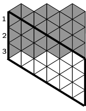
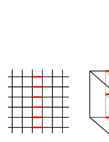
Next, let us take a stacked set of links, 𝒱𝒱\mathcal{V}, which winds around ΛΛ\Lambda in d1𝑑1d-1 periodic directions (𝒱𝒱\mathcal{V} is a closed loop when d=2𝑑2d=2 and a closed surface when d=3𝑑3d=3 on the dual lattice, see fig. 3). Hereafter such 𝒱𝒱\mathcal{V} is called a wall in distinction from a (center) vortex.
Refer to caption
Figure 3: 𝒱𝒱\mathcal{V} in two- and three- dimensions.

The twisted partition function associated to gG𝑔𝐺g\in G is given by

ZΛ(g)[𝒱]xΛdϕxexp(yΛμ=1d[(1δ[𝒱]y,μ)A(ϕy,ϕy+μ^)+δ[𝒱]y,μA(ϕy,gϕy+μ^)]).subscript𝑍Λ𝑔delimited-[]𝒱subscriptproduct𝑥Λ𝑑subscriptitalic-ϕ𝑥subscript𝑦Λsuperscriptsubscript𝜇1𝑑delimited-[]1𝛿subscriptdelimited-[]𝒱𝑦𝜇𝐴subscriptitalic-ϕ𝑦subscriptitalic-ϕ𝑦^𝜇𝛿subscriptdelimited-[]𝒱𝑦𝜇𝐴subscriptitalic-ϕ𝑦𝑔subscriptitalic-ϕ𝑦^𝜇\hskip 30.0ptZ_{\Lambda}(g)[\mathcal{V}]\equiv\displaystyle\int\prod_{x\in\Lambda}d\phi_{x}\ \exp\left(\displaystyle\sum_{y\in\Lambda}\displaystyle\sum_{\mu=1}^{d}\Bigg{[}(1-\delta[\mathcal{V}]_{y,\mu})A(\phi_{y},\phi_{y+\hat{\mu}})+\delta[\mathcal{V}]_{y,\mu}A(\phi_{y},g\phi_{y+\hat{\mu}})\Bigg{]}\right). (62)

The symbol δ[𝒱]y,μ𝛿subscriptdelimited-[]𝒱𝑦𝜇\delta[\mathcal{V}]_{y,\mu} is defined to be =1absent1=1 if the link y,y+μ^𝑦𝑦^𝜇\langle y,y+\hat{\mu}\rangle is contained in 𝒱𝒱\mathcal{V} and =0absent0=0 otherwise. It is not difficult to see that 𝒱𝒱\mathcal{V} cannot be removed from ΛΛ\Lambda by local redefinition of variables ϕgϕitalic-ϕ𝑔italic-ϕ\phi\to g\phi. Let G^^𝐺\hat{G} denote the set of irreducible unitary representations of G𝐺G. The wall creation operators {𝒪(g)[𝒱]|gG}conditional-set𝒪𝑔delimited-[]𝒱𝑔𝐺\{\mathcal{O}(g)[\mathcal{V}]|\,g\in G\} and their duals {R(g)[𝒱]|gG,RG^}conditional-setsubscript𝑅𝑔delimited-[]𝒱formulae-sequence𝑔𝐺𝑅^𝐺\{\mathcal{F}_{R}(g)[\mathcal{V}]|\,g\in G,\,R\in\hat{G}\} are defined as follows:

𝒪(g)[𝒱]delimited-⟨⟩𝒪𝑔delimited-[]𝒱\displaystyle\langle\mathcal{O}(g)[\mathcal{V}]\rangle ZΛ(g)[𝒱]ZΛ,\displaystyle\equiv\displaystyle\frac{\,Z_{\Lambda}(g)[\mathcal{V}]\,^{\mathstrut}}{\,Z_{\Lambda}\,{}_{\mathstrut}}, (63)
𝒪(g)[𝒱]𝒪𝑔delimited-[]𝒱\displaystyle\Longleftrightarrow\ \ \ \mathcal{O}(g)[\mathcal{V}] =exp(yΛμ=1dδ[𝒱]y,μ[A(ϕy,ϕy+μ^)+A(ϕy,gϕy+μ^)]),absentsubscript𝑦Λsuperscriptsubscript𝜇1𝑑𝛿subscriptdelimited-[]𝒱𝑦𝜇delimited-[]𝐴subscriptitalic-ϕ𝑦subscriptitalic-ϕ𝑦^𝜇𝐴subscriptitalic-ϕ𝑦𝑔subscriptitalic-ϕ𝑦^𝜇\displaystyle=\exp\Big{(}\displaystyle\sum_{y\in\Lambda}\displaystyle\sum_{\mu=1}^{d}\delta[\mathcal{V}]_{y,\mu}\Big{[}-A(\phi_{y},\phi_{y+\hat{\mu}})+A(\phi_{y},g\phi_{y+\hat{\mu}})\Big{]}\Big{)}, (64)
R(g)[𝒱]subscript𝑅𝑔delimited-[]𝒱\displaystyle\mathcal{F}_{R}(g)[\mathcal{V}] (dimR)G𝑑x𝒪(gx)[𝒱]χR(x).absentdim𝑅subscript𝐺differential-d𝑥𝒪𝑔𝑥delimited-[]𝒱subscript𝜒𝑅𝑥\displaystyle\equiv({\rm{dim\,}}R)\displaystyle\int_{G}dx\,\mathcal{O}(gx)[\mathcal{V}]\chi_{R}(x). (65)
Lemma 3.

If the walls 𝒱,𝒱𝒱superscript𝒱\mathcal{V},\,\mathcal{V}^{\prime} are homologous 131313Plural walls are called homologous if and only if they wind around the same periodic directions of ΛΛ\Lambda., we have

𝒪(g)[𝒱]𝒪(g)[𝒱]=𝒪(gg)[𝒱]=𝒪(gg)[𝒱],delimited-⟨⟩𝒪𝑔delimited-[]𝒱𝒪superscript𝑔delimited-[]superscript𝒱delimited-⟨⟩𝒪𝑔superscript𝑔delimited-[]𝒱delimited-⟨⟩𝒪superscript𝑔𝑔delimited-[]𝒱\displaystyle\langle\mathcal{O}(g)[\mathcal{V}]\cdot\mathcal{O}(g^{\prime})[\mathcal{V}^{\prime}]\rangle=\langle\mathcal{O}(gg^{\prime})[\mathcal{V}]\rangle=\langle\mathcal{O}(g^{\prime}g)[\mathcal{V}]\rangle, (66)
R(g)[𝒱]R(g)[𝒱]=δRRR(gg)[𝒱]=δRRR(gg)[𝒱],delimited-⟨⟩subscript𝑅𝑔delimited-[]𝒱subscriptsuperscript𝑅superscript𝑔delimited-[]superscript𝒱subscript𝛿𝑅superscript𝑅delimited-⟨⟩subscript𝑅𝑔superscript𝑔delimited-[]𝒱subscript𝛿𝑅superscript𝑅delimited-⟨⟩subscript𝑅superscript𝑔𝑔delimited-[]𝒱\displaystyle\langle\mathcal{F}_{R}(g)[\mathcal{V}]\cdot\mathcal{F}_{R^{\prime}}(g^{\prime})[\mathcal{V}^{\prime}]\rangle=\delta_{RR^{\prime}}\langle\mathcal{F}_{R}(gg^{\prime})[\mathcal{V}]\rangle=\delta_{RR^{\prime}}\langle\mathcal{F}_{R}(g^{\prime}g)[\mathcal{V}]\rangle, (67)
𝒪(g)[𝒱]=RG^R(g)[𝒱],delimited-⟨⟩𝒪𝑔delimited-[]𝒱subscript𝑅^𝐺delimited-⟨⟩subscript𝑅𝑔delimited-[]𝒱\displaystyle\langle\mathcal{O}(g)[\mathcal{V}]\rangle=\displaystyle\sum_{R\in\hat{G}}\langle\mathcal{F}_{R}(g)[\mathcal{V}]\rangle, (68)
1=RG^R(𝟏)[𝒱].1subscript𝑅^𝐺delimited-⟨⟩subscript𝑅1delimited-[]𝒱\displaystyle 1=\displaystyle\sum_{R\in\hat{G}}\langle\mathcal{F}_{R}(\mathbf{1})[\mathcal{V}]\rangle. (69)

(66), (67) imply that 𝒪(g)[𝒱]delimited-⟨⟩𝒪𝑔delimited-[]𝒱\langle\mathcal{O}(g)[\mathcal{V}]\rangle and R(g)[𝒱]delimited-⟨⟩subscript𝑅𝑔delimited-[]𝒱\langle\mathcal{F}_{R}(g)[\mathcal{V}]\rangle are class functions on G𝐺G.

Proof.

(66) is trivial, since the relative position of walls can be reversed owing to the periodic boundary condition (see fig. 4). (67) can be shown by exploiting the invariance of the Haar measure:

R(g)R(g)delimited-⟨⟩subscript𝑅𝑔subscriptsuperscript𝑅superscript𝑔\displaystyle\langle\mathcal{F}_{R}(g)\mathcal{F}_{R^{\prime}}(g^{\prime})\rangle =(dimR)(dimR)G𝑑x𝒪(gx)χR(x)G𝑑y𝒪(gy)χR(y)absentdim𝑅dimsuperscript𝑅delimited-⟨⟩subscript𝐺differential-d𝑥𝒪𝑔𝑥subscript𝜒𝑅𝑥subscript𝐺differential-d𝑦𝒪superscript𝑔𝑦subscript𝜒superscript𝑅𝑦\displaystyle=({\rm{dim\,}}R)({\rm{dim\,}}R^{\prime})\left\langle\displaystyle\int_{G}dx\ \mathcal{O}(gx)\chi_{R}(x)\displaystyle\int_{G}dy\ \mathcal{O}(g^{\prime}y)\chi_{R^{\prime}}(y)\right\rangle (70)
=(dimR)(dimR)G𝑑xG𝑑y𝒪(gxgy)χR(x)χR(y)absentdim𝑅dimsuperscript𝑅subscript𝐺differential-d𝑥subscript𝐺differential-d𝑦delimited-⟨⟩𝒪𝑔𝑥superscript𝑔𝑦subscript𝜒𝑅𝑥subscript𝜒superscript𝑅𝑦\displaystyle=({\rm{dim\,}}R)({\rm{dim\,}}R^{\prime})\displaystyle\int_{G}dx\displaystyle\int_{G}dy\ \langle\mathcal{O}(gxg^{\prime}y)\rangle\chi_{R}(x)\chi_{R^{\prime}}(y) (71)
=(dimR)(dimR)G𝑑x𝒪(x)G𝑑yχR((gg)1xy1)χR(y)absentdim𝑅dimsuperscript𝑅subscript𝐺differential-d𝑥delimited-⟨⟩𝒪𝑥subscript𝐺differential-d𝑦subscript𝜒𝑅superscript𝑔superscript𝑔1𝑥superscript𝑦1subscript𝜒superscript𝑅𝑦\displaystyle=({\rm{dim\,}}R)({\rm{dim\,}}R^{\prime})\displaystyle\int_{G}dx\ \langle\mathcal{O}(x)\rangle\displaystyle\int_{G}dy\ \chi_{R}((gg^{\prime})^{-1}xy^{-1})\chi_{R^{\prime}}(y) (72)
=δRR(dimR)G𝑑x𝒪(x)χR((gg)1x)absentsubscript𝛿𝑅superscript𝑅dim𝑅subscript𝐺differential-d𝑥delimited-⟨⟩𝒪𝑥subscript𝜒𝑅superscript𝑔superscript𝑔1𝑥\displaystyle=\delta_{RR^{\prime}}({\rm{dim\,}}R)\displaystyle\int_{G}dx\ \langle\mathcal{O}(x)\rangle\chi_{R}((gg^{\prime})^{-1}x) (73)
=δRRR(gg).absentsubscript𝛿𝑅superscript𝑅delimited-⟨⟩subscript𝑅𝑔superscript𝑔\displaystyle=\delta_{RR^{\prime}}\langle\mathcal{F}_{R}(gg^{\prime})\rangle. (74)

Finally, (68) is a consequence of the Peter-Weyl theorem [33] according to which any fL2(G)𝑓superscript𝐿2𝐺f\in L^{2}(G) can be represented as

f(g)=RG^(dimR)G𝑑xf(xg)χR(x).𝑓𝑔subscript𝑅^𝐺dim𝑅subscript𝐺differential-d𝑥𝑓𝑥𝑔subscript𝜒𝑅𝑥f(g)=\displaystyle\sum_{R\in\hat{G}}({\rm{dim\,}}R)\displaystyle\int_{G}dx\ f(xg)\chi_{R}(x). (75)

(69) trivially follows from (68). ∎

Refer to caption
Figure 4: Relative position of 𝒱𝒱\mathcal{V} and 𝒱superscript𝒱\mathcal{V}^{\prime} can be reversed by using the periodicity of ΛΛ\Lambda.

Note that (66) cannot be proved in general when other operators are inserted, that is,

𝒪(g)[𝒱]𝒪(g)[𝒱]𝒪(gg)[𝒱]𝒪(gg)[𝒱],delimited-⟨⟩𝒪𝑔delimited-[]𝒱𝒪superscript𝑔delimited-[]superscript𝒱delimited-⟨⟩𝒪𝑔superscript𝑔delimited-[]𝒱delimited-⟨⟩𝒪superscript𝑔𝑔delimited-[]𝒱\langle\mathcal{O}(g)[\mathcal{V}]\cdot\mathcal{O}(g^{\prime})[\mathcal{V}^{\prime}]\dots\rangle\not=\langle\mathcal{O}(gg^{\prime})[\mathcal{V}]\dots\rangle\not=\langle\mathcal{O}(g^{\prime}g)[\mathcal{V}]\dots\rangle, (76)

in general, where \dots denote additional insertions. It is because the proof of (66) involves a sequence of changes of variables. Thus (66) could be proved if inserted operators are invariant under the changes of variables.

Take an arbitrary (d1)𝑑1(d-1)-dimensional hyperplane π𝜋\pi defined by xμ=m,mformulae-sequencesuperscript𝑥𝜇𝑚𝑚x^{\mu}=m,\ m\in\mathbb{Z} with m𝑚m and μ𝜇\mu fixed. Denote by θ𝜃\theta the reflection about π𝜋\pi.

Lemma 4.

If the wall 𝒱𝒱\mathcal{V} seen on the dual lattice is also perpendicular to the xμsuperscript𝑥𝜇x^{\mu}-axis (see the left of fig. 5), we have

θ[𝒪(g)[𝒱]]=𝒪(g1)[𝒱θ],𝜃delimited-[]𝒪𝑔delimited-[]𝒱𝒪superscript𝑔1delimited-[]superscript𝒱𝜃\displaystyle\theta\Big{[}\mathcal{O}(g)[\mathcal{V}]\Big{]}=\mathcal{O}(g^{-1})[\mathcal{V}^{\theta}], (77)
𝒪(g)[𝒱]=𝒪(g1)[𝒱],delimited-⟨⟩𝒪𝑔delimited-[]𝒱delimited-⟨⟩𝒪superscript𝑔1delimited-[]𝒱\displaystyle\langle\mathcal{O}(g)[\mathcal{V}]\rangle=\langle\mathcal{O}(g^{-1})[\mathcal{V}]\rangle, (78)
R(g)[𝒱]=R(g1)[𝒱]¯andR(𝟏)[𝒱]𝐑,formulae-sequencedelimited-⟨⟩subscript𝑅𝑔delimited-[]𝒱¯delimited-⟨⟩subscript𝑅superscript𝑔1delimited-[]𝒱anddelimited-⟨⟩subscript𝑅1delimited-[]𝒱𝐑\displaystyle\langle\mathcal{F}_{R}(g)[\mathcal{V}]\rangle=\overline{\langle\mathcal{F}_{R}({{g^{-1}}})[\mathcal{V}]\rangle}\ \ {\rm{and}}\ \ \langle\mathcal{F}_{R}({\mathbf{1}})[\mathcal{V}]\rangle\in{\mathbf{R}}, (79)
θ[R(g)[𝒱]]=R(g1)[𝒱θ],𝜃delimited-[]subscript𝑅𝑔delimited-[]𝒱subscript𝑅superscript𝑔1delimited-[]superscript𝒱𝜃\displaystyle\theta\Big{[}\mathcal{F}_{R}(g)[\mathcal{V}]\Big{]}=\mathcal{F}_{R}(g^{-1})[\mathcal{V}^{\theta}], (80)

where 𝒱θθ[𝒱]superscript𝒱𝜃𝜃delimited-[]𝒱\mathcal{V}^{\theta}\equiv\theta[\mathcal{V}] and 𝟏1\mathbf{1} denotes the unit element of G𝐺G.

Refer to caption
Figure 5: Insertion of a reflection plane π𝜋\pi.
Proof.

From the right of fig. 5 we observe

θ[A(ϕy,gϕy+μ^)]𝜃delimited-[]𝐴subscriptitalic-ϕ𝑦𝑔subscriptitalic-ϕ𝑦^𝜇\displaystyle\theta\Big{[}A(\phi_{y},g\phi_{y+\hat{\mu}})\Big{]} =A(ϕz+μ^,gϕz)absent𝐴subscriptitalic-ϕ𝑧^𝜇𝑔subscriptitalic-ϕ𝑧\displaystyle=A(\phi_{z+\hat{\mu}},g\phi_{z}) (81)
=A(ϕz,g1ϕz+μ^).absent𝐴subscriptitalic-ϕ𝑧superscript𝑔1subscriptitalic-ϕ𝑧^𝜇\displaystyle=A(\phi_{z},g^{-1}\phi_{z+\hat{\mu}}). (82)

The twist g𝑔g changed to g1superscript𝑔1g^{-1}, hence (77) is proved. (78) immediately follows from (77).

Using (78) we can show

G𝑑x𝒪(gx)[𝒱]χR(x)subscript𝐺differential-d𝑥delimited-⟨⟩𝒪𝑔𝑥delimited-[]𝒱subscript𝜒𝑅𝑥\displaystyle\displaystyle\int_{G}dx\ \langle\mathcal{O}(gx)[\mathcal{V}]\rangle\chi_{R}(x) =G𝑑x𝒪((gx)1)[𝒱]χR(x)absentsubscript𝐺differential-d𝑥delimited-⟨⟩𝒪superscript𝑔𝑥1delimited-[]𝒱subscript𝜒𝑅𝑥\displaystyle=\displaystyle\int_{G}dx\ \langle\mathcal{O}((gx)^{-1})[\mathcal{V}]\rangle\chi_{R}(x) (83)
=G𝑑x𝒪(x1g1)[𝒱]χR(x)absentsubscript𝐺differential-d𝑥delimited-⟨⟩𝒪superscript𝑥1superscript𝑔1delimited-[]𝒱subscript𝜒𝑅𝑥\displaystyle=\displaystyle\int_{G}dx\ \langle\mathcal{O}(x^{-1}g^{-1})[\mathcal{V}]\rangle\chi_{R}(x) (84)
=G𝑑x𝒪(xg1)[𝒱]χR(x1)absentsubscript𝐺differential-d𝑥delimited-⟨⟩𝒪𝑥superscript𝑔1delimited-[]𝒱subscript𝜒𝑅superscript𝑥1\displaystyle=\displaystyle\int_{G}dx\ \langle\mathcal{O}(xg^{-1})[\mathcal{V}]\rangle\chi_{R}(x^{-1}) (85)
=G𝑑x𝒪(g1x)[𝒱]χR(x)¯,absentsubscript𝐺differential-d𝑥delimited-⟨⟩𝒪superscript𝑔1𝑥delimited-[]𝒱¯subscript𝜒𝑅𝑥\displaystyle=\displaystyle\int_{G}dx\ \langle\mathcal{O}(g^{-1}x)[\mathcal{V}]\rangle\overline{\chi_{R}(x)}, (86)

therefore (79) is proved. In the last step we used the fact that R𝑅R is a unitary representation. (80) is obvious from (79). ∎

Though it seems hard to find more properties on general grounds, further nontrivial result can be obtained if we exploit the site-reflection positivity of the measure of (60).

Lemma 5.
𝒪(g)[𝒱],R(𝟏)[𝒱][0,1],delimited-⟨⟩𝒪𝑔delimited-[]𝒱delimited-⟨⟩subscript𝑅1delimited-[]𝒱01\displaystyle\langle\mathcal{O}(g)[\mathcal{V}]\rangle,\ \,\langle\mathcal{F}_{R}(\mathbf{1})[\mathcal{V}]\rangle\ \in[0,1], (87)
|R(g)[𝒱]|R(𝟏)[𝒱].delimited-⟨⟩subscript𝑅𝑔delimited-[]𝒱delimited-⟨⟩subscript𝑅1delimited-[]𝒱\displaystyle|\langle\mathcal{F}_{R}({{g}})[\mathcal{V}]\rangle|\leq\langle\mathcal{F}_{R}({\mathbf{1}})[\mathcal{V}]\rangle. (88)
Proof.

Let 𝒱θθ[𝒱]superscript𝒱𝜃𝜃delimited-[]𝒱\mathcal{V}^{\theta}\equiv\theta[\mathcal{V}]. With the aid of (66), (77) and the Schwarz inequality |F|FθF1/2delimited-⟨⟩𝐹superscriptdelimited-⟨⟩𝐹𝜃𝐹12|\langle F\rangle|\leq\langle F\theta F\rangle^{1/2} we get

𝒪(g)[𝒱]delimited-⟨⟩𝒪𝑔delimited-[]𝒱\displaystyle\langle\mathcal{O}(g)[\mathcal{V}]\rangle 𝒪(g)[𝒱]θ[O(g)[𝒱]]1/2absentsuperscriptdelimited-⟨⟩𝒪𝑔delimited-[]𝒱𝜃delimited-[]𝑂𝑔delimited-[]𝒱12\displaystyle\leq\langle\mathcal{O}(g)[\mathcal{V}]\theta\Big{[}O(g)[\mathcal{V}]\Big{]}\rangle^{1/2} (89)
=𝒪(g)[𝒱]O(g1)[𝒱θ]1/2=1.absentsuperscriptdelimited-⟨⟩𝒪𝑔delimited-[]𝒱𝑂superscript𝑔1delimited-[]superscript𝒱𝜃121\displaystyle=\langle\mathcal{O}(g)[\mathcal{V}]O(g^{-1})[\mathcal{V}^{\theta}]\rangle^{1/2}=1. (90)

Next, using (67) and (80) yields

R(𝟏)[𝒱]delimited-⟨⟩subscript𝑅1delimited-[]𝒱\displaystyle\langle\mathcal{F}_{R}(\mathbf{1})[\mathcal{V}]\rangle =R(𝟏)[𝒱]R(𝟏)[𝒱θ]absentdelimited-⟨⟩subscript𝑅1delimited-[]𝒱subscript𝑅1delimited-[]superscript𝒱𝜃\displaystyle=\langle\mathcal{F}_{R}(\mathbf{1})[\mathcal{V}]\cdot\mathcal{F}_{R}(\mathbf{1})[\mathcal{V}^{\theta}]\rangle (91)
=R(𝟏)[𝒱]θ[R(𝟏)[𝒱]]0.absentdelimited-⟨⟩subscript𝑅1delimited-[]𝒱𝜃delimited-[]subscript𝑅1delimited-[]𝒱0\displaystyle=\langle\mathcal{F}_{R}(\mathbf{1})[\mathcal{V}]\cdot\theta\Big{[}\mathcal{F}_{R}(\mathbf{1})[\mathcal{V}]\Big{]}\rangle\geq 0. (92)

(92) combined with (69) yields (87).

Finally, to show (88) we use (80) and the Schwarz inequality |FθG|FθF1/2GθG1/2delimited-⟨⟩𝐹𝜃𝐺superscriptdelimited-⟨⟩𝐹𝜃𝐹12superscriptdelimited-⟨⟩𝐺𝜃𝐺12|\langle F\theta G\rangle|\leq\langle F\theta F\rangle^{1/2}\langle G\theta G\rangle^{1/2} as follows: letting 𝒱superscript𝒱\mathcal{V}^{\prime} denote a wall homologous to 𝒱𝒱\mathcal{V}, we have

|R(g)[𝒱]|delimited-⟨⟩subscript𝑅𝑔delimited-[]𝒱\displaystyle|\langle\mathcal{F}_{R}(g)[\mathcal{V}]\rangle| =|R(g)[𝒱]R(𝟏)[𝒱]|absentdelimited-⟨⟩subscript𝑅𝑔delimited-[]𝒱subscript𝑅1delimited-[]superscript𝒱\displaystyle=|\langle\mathcal{F}_{R}(g)[\mathcal{V}]\mathcal{F}_{R}({\mathbf{1}})[\mathcal{V}^{\prime}]\rangle| (93)
R(g)[𝒱]R(g1)[𝒱θ]1/2R(𝟏)[𝒱]R(𝟏)[𝒱θ]1/2absentsuperscriptdelimited-⟨⟩subscript𝑅𝑔delimited-[]𝒱subscript𝑅superscript𝑔1delimited-[]superscript𝒱𝜃12superscriptdelimited-⟨⟩subscript𝑅1delimited-[]superscript𝒱subscript𝑅1delimited-[]superscript𝒱𝜃12\displaystyle\leq\langle\mathcal{F}_{R}(g)[\mathcal{V}]\mathcal{F}_{R}(g^{-1})[\mathcal{V}^{\theta}]\rangle^{1/2}\langle\mathcal{F}_{R}({\mathbf{1}})[\mathcal{V}^{\prime}]\mathcal{F}_{R}({\mathbf{1}})[\mathcal{V}^{\prime\theta}]\rangle^{1/2} (94)
=R(𝟏)[𝒱]1/2R(𝟏)[𝒱]1/2absentsuperscriptdelimited-⟨⟩subscript𝑅1delimited-[]𝒱12superscriptdelimited-⟨⟩subscript𝑅1delimited-[]superscript𝒱12\displaystyle=\langle\mathcal{F}_{R}({\mathbf{1}})[\mathcal{V}]\rangle^{1/2}\langle\mathcal{F}_{R}({\mathbf{1}})[\mathcal{V}^{\prime}]\rangle^{1/2} (95)
=R(𝟏)[𝒱].absentdelimited-⟨⟩subscript𝑅1delimited-[]𝒱\displaystyle=\langle\mathcal{F}_{R}({\mathbf{1}})[\mathcal{V}]\rangle. (96)

3.2 TY inequality in spin systems

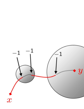
A natural counterpart in spin systems of Wilson loops in LGT is a two-point correlation function Γ(ϕx,ϕy)Γsubscriptitalic-ϕ𝑥subscriptitalic-ϕ𝑦\Gamma(\phi_{x},\phi_{y}) as explained in the Introduction. ΓΓ\Gamma will decay exponentially with a mass gap (in symmetric phase) while decay algebraically without a mass gap (in a spontaneous symmetry breaking phase or Kosterlitz-Thouless-type phase). If 𝒪(g)delimited-⟨⟩𝒪𝑔\langle\mathcal{O}(g)\rangle defined above converges to 1 in the thermodynamic limit, it follows that arbitrarily huge domain walls grow with little cost and eventually drive the system to the disordered phase with a mass gap (see fig. 6). 𝒪(g)1(|Λ|)delimited-⟨⟩𝒪𝑔1Λ\langle\mathcal{O}(g)\rangle\to 1\ \,(|\Lambda|\to\infty) can also be regarded as a sign of insensitivity of the system to boundary conditions, which indicates the absence of massless particles.

If (as in Ising-like models) we assume that the intersection of a correlation line with a wall changes the sign of ΓΓ\Gamma, a small closed wall gives no contribution ((1)2=1superscript121(-1)^{2}=1) while a huge wall can give (1)1(-1). If each link on the correlation line of total length L𝐿L is assumed to intersect with a wall independently with probability p𝑝p, we obtain

Γk=0L(Lk)(1)kpk(1p)Lk=(12p)LemL,m=log(12p).formulae-sequencesimilar-todelimited-⟨⟩Γsuperscriptsubscript𝑘0𝐿matrix𝐿𝑘superscript1𝑘superscript𝑝𝑘superscript1𝑝𝐿𝑘superscript12𝑝𝐿similar-tosuperscript𝑒𝑚𝐿𝑚12𝑝\langle\Gamma\rangle\sim\displaystyle\sum_{k=0}^{L}\begin{pmatrix}L\\ k\end{pmatrix}(-1)^{k}p^{k}(1-p)^{L-k}=(1-2p)^{L}\sim e^{-mL},\hskip 30.0ptm=-\log(1-2p). (97)
Refer to caption
Figure 6: Disorder being caused by walls.

Our goal in this section is to elevate the above heuristic relation of disorder and a mass gap to a mathematically rigorous inequality.

Suppose that the explicit form of the correlation function ΓΓ\Gamma is given by

Γμ(x;n)=αfα(ϕx)fα(ϕx+nμ^)¯,n𝐍,formulae-sequencesubscriptΓ𝜇𝑥𝑛subscript𝛼subscript𝑓𝛼subscriptitalic-ϕ𝑥¯subscript𝑓𝛼subscriptitalic-ϕ𝑥𝑛^𝜇𝑛𝐍\Gamma_{\mu}(x;n)=\displaystyle\sum_{\alpha}f_{\alpha}(\phi_{x})\overline{f_{\alpha}(\phi_{x+n\hat{\mu}})},\hskip 30.0ptn\in\mathbf{N}, (98)

where f𝑓f is an arbitrary function from the order-parameter space to 𝐂𝐂\mathbf{C} endowed with generic indices {α}𝛼\{\alpha\}. Here fαsubscript𝑓𝛼f_{\alpha} is meant to specify, for example, the α𝛼\alpha-th component of a vector spin in O(N)𝑂𝑁O(N)-like models, or the α𝛼\alpha-th matrix element of a matrix spin in PCM-like models. Note that Γμ(x;n)delimited-⟨⟩subscriptΓ𝜇𝑥𝑛\langle\Gamma_{\mu}(x;n)\rangle is independent of x𝑥x due to the translational invariance of the system. An important requirement on ΓμsubscriptΓ𝜇\Gamma_{\mu} is its invariance under G𝐺G :

αfα(ϕx)fα(ϕx+nμ^)¯=αfα(gϕx)fα(gϕx+nμ^)¯,gG.formulae-sequencesubscript𝛼subscript𝑓𝛼subscriptitalic-ϕ𝑥¯subscript𝑓𝛼subscriptitalic-ϕ𝑥𝑛^𝜇subscript𝛼subscript𝑓𝛼𝑔subscriptitalic-ϕ𝑥¯subscript𝑓𝛼𝑔subscriptitalic-ϕ𝑥𝑛^𝜇𝑔𝐺\displaystyle\sum_{\alpha}f_{\alpha}(\phi_{x})\overline{f_{\alpha}(\phi_{x+n\hat{\mu}})}=\displaystyle\sum_{\alpha}f_{\alpha}(g\phi_{x})\overline{f_{\alpha}(g\phi_{x+n\hat{\mu}})},\hskip 20.0ptg\in G. (99)

Another requirement, which is truly indispensable for all the following development, is

Gdgfα(gϕ)=0forϕ.\displaystyle\int_{G}dg\,f_{\alpha}(g\phi)=0\ \ \ \ \ {\rm{for}}\ \ ^{\forall}\phi. (100)

If (100) were not satisfied, we should replace fα(ϕ)subscript𝑓𝛼italic-ϕf_{\alpha}(\phi) by fα(ϕ)fα(ϕ)G𝑑gfα(gϕ)subscriptsuperscript𝑓𝛼italic-ϕsubscript𝑓𝛼italic-ϕsubscript𝐺differential-d𝑔subscript𝑓𝛼𝑔italic-ϕf^{\prime}_{\alpha}(\phi)\equiv f_{\alpha}(\phi)-\displaystyle\int_{G}dg\,f_{\alpha}(g\phi).

Theorem 5.

Assume (99), (100) and the existence of k𝐍𝑘𝐍k\in\mathbf{N} such that Lμ=2knsubscript𝐿𝜇superscript2𝑘𝑛L_{\mu}=2^{k}n, with Lμsubscript𝐿𝜇L_{\mu} the extent of ΛΛ\Lambda in the xμsuperscript𝑥𝜇x^{\mu}-direction.141414 It does not seem to be very restrictive; in general we believe in the existence of the limit Lμsubscript𝐿𝜇L_{\mu}\to\infty for physical observables independent of the way we take Lμsubscript𝐿𝜇L_{\mu}\to\infty. Then we have

|Γμ(x;n)|Γμ(x;0)2{Γμ(x;0)2Γμ(x;0)2}n/Lμ{1G𝑑g𝒪(g)[𝒱]}n/Lμ,superscriptdelimited-⟨⟩subscriptΓ𝜇𝑥𝑛absentsubscriptdelimited-⟨⟩subscriptΓ𝜇𝑥0absent2superscriptsuperscriptdelimited-⟨⟩subscriptΓ𝜇superscript𝑥02absentsubscriptsuperscriptdelimited-⟨⟩subscriptΓ𝜇𝑥02absent𝑛subscript𝐿𝜇superscript1subscript𝐺differential-d𝑔delimited-⟨⟩𝒪𝑔delimited-[]𝒱𝑛subscript𝐿𝜇\displaystyle\frac{\,|\langle\Gamma_{\mu}(x;n)\rangle|\,^{\mathstrut}}{\,\langle\Gamma_{\mu}(x;0)\rangle\,_{\mathstrut}}\leq 2\left\{\displaystyle\frac{\,\langle\Gamma_{\mu}(x;0)^{2}\rangle\,^{\mathstrut}}{\,\langle\Gamma_{\mu}(x;0)\rangle^{2}\,_{\mathstrut}}\right\}^{n/L_{\mu}}\left\{1-\displaystyle\int_{G}dg\,\langle\mathcal{O}(g)[\mathcal{V}]\rangle\right\}^{n/L_{\mu}}, (101)

where 𝒱𝒱\mathcal{V} is a wall perpendicular to the xμsuperscript𝑥𝜇x^{\mu}-direction .1515150<Γμ(n)0delimited-⟨⟩subscriptΓ𝜇𝑛0<\langle\Gamma_{\mu}(n)\rangle can be proved by the site-reflection positivity if n𝑛n is even.

Proof.

We first decompose the correlation function into two parts:

Γμ(x;n)=Γμ(x;n)(1T(𝟏)[𝒱])+Γμ(x;n)T(𝟏)[𝒱],delimited-⟨⟩subscriptΓ𝜇𝑥𝑛delimited-⟨⟩subscriptΓ𝜇𝑥𝑛1subscript𝑇1delimited-[]𝒱delimited-⟨⟩subscriptΓ𝜇𝑥𝑛subscript𝑇1delimited-[]𝒱\langle\Gamma_{\mu}(x;n)\rangle=\langle\Gamma_{\mu}(x;n)(1-\mathcal{F}_{T}(\mathbf{1})[\mathcal{V}])\rangle+\langle\Gamma_{\mu}(x;n)\mathcal{F}_{T}(\mathbf{1})[\mathcal{V}]\rangle, (102)

where T𝑇T denotes the trivial representation, i.e. T(𝟏)[𝒱]=G𝑑g𝒪(g)[𝒱]subscript𝑇1delimited-[]𝒱subscript𝐺differential-d𝑔𝒪𝑔delimited-[]𝒱\mathcal{F}_{T}(\mathbf{1})[\mathcal{V}]=\displaystyle\int_{G}dg\,\mathcal{O}(g)[\mathcal{V}]. Our basic idea here is to apply the Schwarz inequality

|FθG|FθF1/2GθG1/2delimited-⟨⟩𝐹𝜃𝐺superscriptdelimited-⟨⟩𝐹𝜃𝐹12superscriptdelimited-⟨⟩𝐺𝜃𝐺12|\langle F\theta G\rangle|\leq\langle F\theta F\rangle^{1/2}\langle G\theta G\rangle^{1/2} (103)

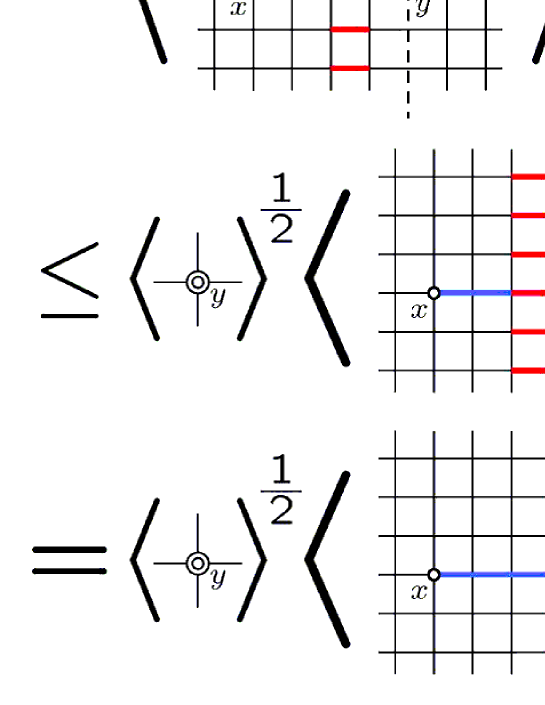
to each term of (102). The procedure afterward is represented graphically in fig. 7 where (1T(𝟏)[𝒱])1subscript𝑇1delimited-[]𝒱(1-\mathcal{F}_{T}(\mathbf{1})[\mathcal{V}]) is indicated by red segments and a blue line is drawn to guide the eye. Let yx+nμ^𝑦𝑥𝑛^𝜇y\equiv x+n\hat{\mu} and zx+2nμ^𝑧𝑥2𝑛^𝜇z\equiv x+2n\hat{\mu}. Consider a reflection θ𝜃\theta about π𝜋\pi (a hyperplane perpendicular to μ^^𝜇\hat{\mu} and lying at y𝑦y ). Using (67), (80), (99) and (103) we get

|Γμ(x;n)(1T(𝟏)[𝒱])|Γμ(x;0)superscriptdelimited-⟨⟩subscriptΓ𝜇𝑥𝑛1subscript𝑇1delimited-[]𝒱absentsubscriptdelimited-⟨⟩subscriptΓ𝜇𝑥0absent\displaystyle\displaystyle\frac{\,|\langle\Gamma_{\mu}(x;n)(1-\mathcal{F}_{T}(\mathbf{1})[\mathcal{V}])\rangle|\,^{\mathstrut}}{\,\langle\Gamma_{\mu}(x;0)\rangle\,_{\mathstrut}} (104)
=\displaystyle=\  1Γμ(x;0)|αfα(ϕx)fα(ϕy)¯(1T(𝟏)[𝒱])|superscript1absentsubscriptdelimited-⟨⟩subscriptΓ𝜇𝑥0absentsubscript𝛼delimited-⟨⟩subscript𝑓𝛼subscriptitalic-ϕ𝑥¯subscript𝑓𝛼subscriptitalic-ϕ𝑦1subscript𝑇1delimited-[]𝒱\displaystyle\displaystyle\frac{\,1\,^{\mathstrut}}{\,\langle\Gamma_{\mu}(x;0)\rangle\,_{\mathstrut}}\Big{|}\displaystyle\sum_{\alpha}\langle f_{\alpha}(\phi_{x})\overline{f_{\alpha}(\phi_{y})}(1-\mathcal{F}_{T}(\mathbf{1})[\mathcal{V}])\rangle\Big{|} (105)
\displaystyle\leq\  1Γμ(x;0)αfα(ϕx)(1T(𝟏)[𝒱])θ[fα(ϕx)(1T(𝟏)[𝒱])]1/2fα(ϕy)¯θ[fα(ϕy)¯]1/2superscript1absentsubscriptdelimited-⟨⟩subscriptΓ𝜇𝑥0absentsubscript𝛼superscriptdelimited-⟨⟩subscript𝑓𝛼subscriptitalic-ϕ𝑥1subscript𝑇1delimited-[]𝒱𝜃delimited-[]subscript𝑓𝛼subscriptitalic-ϕ𝑥1subscript𝑇1delimited-[]𝒱12superscriptdelimited-⟨⟩¯subscript𝑓𝛼subscriptitalic-ϕ𝑦𝜃delimited-[]¯subscript𝑓𝛼subscriptitalic-ϕ𝑦12\displaystyle\displaystyle\frac{\,1\,^{\mathstrut}}{\,\langle\Gamma_{\mu}(x;0)\rangle\,_{\mathstrut}}\displaystyle\sum_{\alpha}\Big{\langle}f_{\alpha}(\phi_{x})(1-\mathcal{F}_{T}(\mathbf{1})[\mathcal{V}])\cdot\theta\Big{[}f_{\alpha}(\phi_{x})(1-\mathcal{F}_{T}(\mathbf{1})[\mathcal{V}])\Big{]}\Big{\rangle}^{1/2}\Big{\langle}\overline{f_{\alpha}(\phi_{y})}\theta\Big{[}\overline{f_{\alpha}(\phi_{y})}\Big{]}\Big{\rangle}^{1/2} (106)
=\displaystyle=\  1Γμ(x;0)αfα(ϕx)(1T(𝟏)[𝒱])fα(ϕz)¯(1T(𝟏)[𝒱θ])1/2fα(ϕy)¯fα(ϕy)1/2superscript1absentsubscriptdelimited-⟨⟩subscriptΓ𝜇𝑥0absentsubscript𝛼superscriptdelimited-⟨⟩subscript𝑓𝛼subscriptitalic-ϕ𝑥1subscript𝑇1delimited-[]𝒱¯subscript𝑓𝛼subscriptitalic-ϕ𝑧1subscript𝑇1delimited-[]superscript𝒱𝜃12superscriptdelimited-⟨⟩¯subscript𝑓𝛼subscriptitalic-ϕ𝑦subscript𝑓𝛼subscriptitalic-ϕ𝑦12\displaystyle\displaystyle\frac{\,1\,^{\mathstrut}}{\,\langle\Gamma_{\mu}(x;0)\rangle\,_{\mathstrut}}\displaystyle\sum_{\alpha}\big{\langle}f_{\alpha}(\phi_{x})(1-\mathcal{F}_{T}(\mathbf{1})[\mathcal{V}])\overline{f_{\alpha}(\phi_{z})}(1-\mathcal{F}_{T}(\mathbf{1})[\mathcal{V}^{\theta}])\big{\rangle}^{1/2}\big{\langle}\overline{f_{\alpha}(\phi_{y})}f_{\alpha}(\phi_{y})\big{\rangle}^{1/2} (107)
\displaystyle\leq\  1Γμ(x;0)αfα(ϕx)fα(ϕz)¯(1T(𝟏)[𝒱])1/2αfα(ϕy)¯fα(ϕy)1/2superscript1absentsubscriptdelimited-⟨⟩subscriptΓ𝜇𝑥0absentsuperscriptdelimited-⟨⟩subscript𝛼subscript𝑓𝛼subscriptitalic-ϕ𝑥¯subscript𝑓𝛼subscriptitalic-ϕ𝑧1subscript𝑇1delimited-[]𝒱12superscriptdelimited-⟨⟩subscript𝛼¯subscript𝑓𝛼subscriptitalic-ϕ𝑦subscript𝑓𝛼subscriptitalic-ϕ𝑦12\displaystyle\displaystyle\frac{\,1\,^{\mathstrut}}{\,\langle\Gamma_{\mu}(x;0)\rangle\,_{\mathstrut}}\Big{\langle}\displaystyle\sum_{\alpha}f_{\alpha}(\phi_{x})\overline{f_{\alpha}(\phi_{z})}(1-\mathcal{F}_{T}(\mathbf{1})[\mathcal{V}])\Big{\rangle}^{1/2}\Big{\langle}\displaystyle\sum_{\alpha}\overline{f_{\alpha}(\phi_{y})}f_{\alpha}(\phi_{y})\Big{\rangle}^{1/2} (108)
=\displaystyle=\ {Γμ(x;2n)(1T(𝟏)[𝒱])Γμ(x;0)}1/2.superscriptsuperscriptdelimited-⟨⟩subscriptΓ𝜇𝑥2𝑛1subscript𝑇1delimited-[]𝒱absentsubscriptdelimited-⟨⟩subscriptΓ𝜇𝑥0absent12\displaystyle\left\{\displaystyle\frac{\,\langle\Gamma_{\mu}(x;2n)(1-\mathcal{F}_{T}(\mathbf{1})[\mathcal{V}])\rangle\,^{\mathstrut}}{\,\langle\Gamma_{\mu}(x;0)\rangle\,_{\mathstrut}}\right\}^{1/2}. (109)
Refer to caption
Figure 7: Schwarz inequality enables us to double the distance of points in the correlation function.

Iterating this procedure for (k1)𝑘1(k-1) times yields (note Lμ=2knsubscript𝐿𝜇superscript2𝑘𝑛L_{\mu}=2^{k}n)

|Γμ(n)(1T(𝟏)[𝒱])|Γμ(0){Γμ(Lμ/2)(1T(𝟏)[𝒱])Γμ(0)}2n/Lμ.superscriptdelimited-⟨⟩subscriptΓ𝜇𝑛1subscript𝑇1delimited-[]𝒱absentsubscriptdelimited-⟨⟩subscriptΓ𝜇0absentsuperscriptsuperscriptdelimited-⟨⟩subscriptΓ𝜇subscript𝐿𝜇21subscript𝑇1delimited-[]𝒱absentsubscriptdelimited-⟨⟩subscriptΓ𝜇0absent2𝑛subscript𝐿𝜇\displaystyle\frac{\,|\langle\Gamma_{\mu}(n)(1-\mathcal{F}_{T}(\mathbf{1})[\mathcal{V}])\rangle|\,^{\mathstrut}}{\,\langle\Gamma_{\mu}(0)\rangle\,_{\mathstrut}}\leq\left\{\displaystyle\frac{\,\langle\Gamma_{\mu}(L_{\mu}/2)(1-\mathcal{F}_{T}(\mathbf{1})[\mathcal{V}])\rangle\,^{\mathstrut}}{\,\langle\Gamma_{\mu}(0)\rangle\,_{\mathstrut}}\right\}^{2n/L_{\mu}}. (110)
Refer to caption
Figure 8: θ𝜃\theta is a reflection about π𝜋\pi that bisects ΛΛ\Lambda. Here ΛΛ\Lambda is shown as a one-dimensional chain for simplicity.

Finally, let us define the reflection θ𝜃\theta w.r.t. the hyperplane π𝜋\pi which runs through x𝑥x and x+(Lμ/2)μ^𝑥subscript𝐿𝜇2^𝜇x+(L_{\mu}/2)\hat{\mu} (thus θ[x]=x𝜃delimited-[]𝑥𝑥\theta[x]=x and θ[x+(Lμ/2)μ^]=x+(Lμ/2)μ^𝜃delimited-[]𝑥subscript𝐿𝜇2^𝜇𝑥subscript𝐿𝜇2^𝜇\theta[x+(L_{\mu}/2)\hat{\mu}]=x+(L_{\mu}/2)\hat{\mu}, see fig.8). Then we obtain

Γμ(x;Lμ/2)(1T(𝟏)[𝒱])Γμ(x;0)superscriptdelimited-⟨⟩subscriptΓ𝜇𝑥subscript𝐿𝜇21subscript𝑇1delimited-[]𝒱absentsubscriptdelimited-⟨⟩subscriptΓ𝜇𝑥0absent\displaystyle\displaystyle\frac{\,\langle\Gamma_{\mu}(x;L_{\mu}/2)(1-\mathcal{F}_{T}(\mathbf{1})[\mathcal{V}])\rangle\,^{\mathstrut}}{\,\langle\Gamma_{\mu}(x;0)\rangle\,_{\mathstrut}} (111)
\displaystyle\leq\ Γμ(x;Lμ/2)θ[Γμ(x;Lμ/2)]1/2(1T(𝟏)[𝒱])(1T(𝟏)[𝒱θ])1/2Γμ(x;0)\displaystyle\displaystyle\frac{\,\langle\Gamma_{\mu}(x;L_{\mu}/2)\theta[\Gamma_{\mu}(x;L_{\mu}/2)]\rangle^{1/2}\langle(1-\mathcal{F}_{T}(\mathbf{1})[\mathcal{V}])(1-\mathcal{F}_{T}(\mathbf{1})[\mathcal{V}^{\theta}])\rangle^{1/2}\,{}^{\mathstrut}}{\,\langle\Gamma_{\mu}(x;0)\rangle\,_{\mathstrut}} (112)
\displaystyle\leq\ Γμ(x;0)21/2{1T(𝟏)[𝒱]}1/2Γμ(x;0)(={Γμ(x;0)2Γμ(x;0)2}1/2{1T(𝟏)[𝒱]}1/2),\displaystyle\displaystyle\frac{\,\langle\Gamma_{\mu}(x;0)^{2}\rangle^{1/2}\left\{1-\langle\mathcal{F}_{T}(\mathbf{1})[\mathcal{V}]\rangle\right\}^{1/2}\,{}^{\mathstrut}}{\,\langle\Gamma_{\mu}(x;0)\rangle\,_{\mathstrut}}\left(=\left\{\displaystyle\frac{\,\langle\Gamma_{\mu}(x;0)^{2}\rangle\,^{\mathstrut}}{\,\langle\Gamma_{\mu}(x;0)\rangle^{2}\,_{\mathstrut}}\right\}^{1/2}\left\{1-\langle\mathcal{F}_{T}(\mathbf{1})[\mathcal{V}]\rangle\right\}^{1/2}\right), (113)

thus

0Γμ(x;n)(1T(𝟏)[𝒱])Γμ(x;0){Γμ(x;0)2Γμ(x;0)2}n/Lμ{1T(𝟏)[𝒱]}n/Lμ.0superscriptdelimited-⟨⟩subscriptΓ𝜇𝑥𝑛1subscript𝑇1delimited-[]𝒱absentsubscriptdelimited-⟨⟩subscriptΓ𝜇𝑥0absentsuperscriptsuperscriptdelimited-⟨⟩subscriptΓ𝜇superscript𝑥02absentsubscriptsuperscriptdelimited-⟨⟩subscriptΓ𝜇𝑥02absent𝑛subscript𝐿𝜇superscript1delimited-⟨⟩subscript𝑇1delimited-[]𝒱𝑛subscript𝐿𝜇0\leq\displaystyle\frac{\,\langle\Gamma_{\mu}(x;n)(1-\mathcal{F}_{T}(\mathbf{1})[\mathcal{V}])\rangle\,^{\mathstrut}}{\,\langle\Gamma_{\mu}(x;0)\rangle\,_{\mathstrut}}\leq\left\{\displaystyle\frac{\,\langle\Gamma_{\mu}(x;0)^{2}\rangle\,^{\mathstrut}}{\,\langle\Gamma_{\mu}(x;0)\rangle^{2}\,_{\mathstrut}}\right\}^{n/L_{\mu}}\left\{1-\langle\mathcal{F}_{T}(\mathbf{1})[\mathcal{V}]\rangle\right\}^{n/L_{\mu}}. (114)

In deriving (113) we used Γμ(x;Lμ/2)θ[Γμ(x;Lμ/2)]Γμ(x;0)2delimited-⟨⟩subscriptΓ𝜇𝑥subscript𝐿𝜇2𝜃delimited-[]subscriptΓ𝜇𝑥subscript𝐿𝜇2delimited-⟨⟩subscriptΓ𝜇superscript𝑥02\langle\Gamma_{\mu}(x;L_{\mu}/2)\theta[\Gamma_{\mu}(x;L_{\mu}/2)]\rangle\leq\langle\Gamma_{\mu}(x;0)^{2}\rangle. This can be shown as follows:

Γμ(x;Lμ/2)θ[Γμ(x;Lμ/2)]delimited-⟨⟩subscriptΓ𝜇𝑥subscript𝐿𝜇2𝜃delimited-[]subscriptΓ𝜇𝑥subscript𝐿𝜇2\displaystyle\langle\Gamma_{\mu}(x;L_{\mu}/2)\theta[\Gamma_{\mu}(x;L_{\mu}/2)]\rangle (115)
=\displaystyle=\ α,βfα(ϕx)fα(ϕx+(Lμ/2)μ^)¯θ[fβ(ϕx)fβ(ϕx+(Lμ/2)μ^)¯]subscript𝛼𝛽delimited-⟨⟩subscript𝑓𝛼subscriptitalic-ϕ𝑥¯subscript𝑓𝛼subscriptitalic-ϕ𝑥subscript𝐿𝜇2^𝜇𝜃delimited-[]subscript𝑓𝛽subscriptitalic-ϕ𝑥¯subscript𝑓𝛽subscriptitalic-ϕ𝑥subscript𝐿𝜇2^𝜇\displaystyle\displaystyle\sum_{\alpha,\beta}\Big{\langle}f_{\alpha}(\phi_{x})\overline{f_{\alpha}(\phi_{x+(L_{\mu}/2)\hat{\mu}})}\cdot\theta\Big{[}f_{\beta}(\phi_{x})\overline{f_{\beta}(\phi_{x+(L_{\mu}/2)\hat{\mu}})}\Big{]}\Big{\rangle} (116)
=\displaystyle=\ α,βfα(ϕx)fα(ϕx+(Lμ/2)μ^)¯fβ(ϕx)¯fβ(ϕx+(Lμ/2)μ^)subscript𝛼𝛽delimited-⟨⟩subscript𝑓𝛼subscriptitalic-ϕ𝑥¯subscript𝑓𝛼subscriptitalic-ϕ𝑥subscript𝐿𝜇2^𝜇¯subscript𝑓𝛽subscriptitalic-ϕ𝑥subscript𝑓𝛽subscriptitalic-ϕ𝑥subscript𝐿𝜇2^𝜇\displaystyle\displaystyle\sum_{\alpha,\beta}\big{\langle}f_{\alpha}(\phi_{x})\overline{f_{\alpha}(\phi_{x+(L_{\mu}/2)\hat{\mu}})}\ \overline{f_{\beta}(\phi_{x})}f_{\beta}(\phi_{x+(L_{\mu}/2)\hat{\mu}})\big{\rangle} (117)
\displaystyle\leq\ α,βfα(ϕx)fβ(ϕx)¯θ[fα(ϕx)fβ(ϕx)¯]1/2fα(ϕx+(Lμ/2)μ^)¯fβ(ϕx+(Lμ/2)μ^)θ[fα(ϕx+(Lμ/2)μ^)¯fβ(ϕx+(Lμ/2)μ^)]1/2subscript𝛼𝛽superscriptdelimited-⟨⟩subscript𝑓𝛼subscriptitalic-ϕ𝑥¯subscript𝑓𝛽subscriptitalic-ϕ𝑥𝜃delimited-[]subscript𝑓𝛼subscriptitalic-ϕ𝑥¯subscript𝑓𝛽subscriptitalic-ϕ𝑥12superscriptdelimited-⟨⟩¯subscript𝑓𝛼subscriptitalic-ϕ𝑥subscript𝐿𝜇2^𝜇subscript𝑓𝛽subscriptitalic-ϕ𝑥subscript𝐿𝜇2^𝜇𝜃delimited-[]¯subscript𝑓𝛼subscriptitalic-ϕ𝑥subscript𝐿𝜇2^𝜇subscript𝑓𝛽subscriptitalic-ϕ𝑥subscript𝐿𝜇2^𝜇12\displaystyle\displaystyle\sum_{\alpha,\beta}\Big{\langle}f_{\alpha}(\phi_{x})\overline{f_{\beta}(\phi_{x})}\cdot\theta\Big{[}f_{\alpha}(\phi_{x})\overline{f_{\beta}(\phi_{x})}\Big{]}\Big{\rangle}^{1/2}\Big{\langle}\overline{f_{\alpha}(\phi_{x+(L_{\mu}/2)\hat{\mu}})}f_{\beta}(\phi_{x+(L_{\mu}/2)\hat{\mu}})\cdot\theta\Big{[}\overline{f_{\alpha}(\phi_{x+(L_{\mu}/2)\hat{\mu}})}f_{\beta}(\phi_{x+(L_{\mu}/2)\hat{\mu}})\Big{]}\Big{\rangle}^{1/2} (118)
=\displaystyle=\ α,β|fα(ϕx)|2|fβ(ϕx)|21/2|fα(ϕx+(Lμ/2)μ^)|2|fβ(ϕx+(Lμ/2)μ^)|21/2subscript𝛼𝛽superscriptdelimited-⟨⟩superscriptsubscript𝑓𝛼subscriptitalic-ϕ𝑥2superscriptsubscript𝑓𝛽subscriptitalic-ϕ𝑥212superscriptdelimited-⟨⟩superscriptsubscript𝑓𝛼subscriptitalic-ϕ𝑥subscript𝐿𝜇2^𝜇2superscriptsubscript𝑓𝛽subscriptitalic-ϕ𝑥subscript𝐿𝜇2^𝜇212\displaystyle\displaystyle\sum_{\alpha,\beta}\langle|f_{\alpha}(\phi_{x})|^{2}|f_{\beta}(\phi_{x})|^{2}\rangle^{1/2}\langle|f_{\alpha}(\phi_{x+(L_{\mu}/2)\hat{\mu}})|^{2}|f_{\beta}(\phi_{x+(L_{\mu}/2)\hat{\mu}})|^{2}\rangle^{1/2} (119)
\displaystyle\leq\ α,β|fα(ϕx)|2|fβ(ϕx)|21/2α,β|fα(ϕx+(Lμ/2)μ^)|2|fβ(ϕx+(Lμ/2)μ^)|21/2superscriptdelimited-⟨⟩subscript𝛼𝛽superscriptsubscript𝑓𝛼subscriptitalic-ϕ𝑥2superscriptsubscript𝑓𝛽subscriptitalic-ϕ𝑥212superscriptdelimited-⟨⟩subscript𝛼𝛽superscriptsubscript𝑓𝛼subscriptitalic-ϕ𝑥subscript𝐿𝜇2^𝜇2superscriptsubscript𝑓𝛽subscriptitalic-ϕ𝑥subscript𝐿𝜇2^𝜇212\displaystyle\Big{\langle}\displaystyle\sum_{\alpha,\beta}|f_{\alpha}(\phi_{x})|^{2}|f_{\beta}(\phi_{x})|^{2}\Big{\rangle}^{1/2}\Big{\langle}\displaystyle\sum_{\alpha,\beta}|f_{\alpha}(\phi_{x+(L_{\mu}/2)\hat{\mu}})|^{2}|f_{\beta}(\phi_{x+(L_{\mu}/2)\hat{\mu}})|^{2}\Big{\rangle}^{1/2} (120)
=\displaystyle=\ Γμ(x;0)21/2Γμ(x+(Lμ/2);0)21/2=Γμ(x;0)2.superscriptdelimited-⟨⟩subscriptΓ𝜇superscript𝑥0212superscriptdelimited-⟨⟩subscriptΓ𝜇superscript𝑥subscript𝐿𝜇20212delimited-⟨⟩subscriptΓ𝜇superscript𝑥02\displaystyle\langle\Gamma_{\mu}(x;0)^{2}\rangle^{1/2}\langle\Gamma_{\mu}(x+(L_{\mu}/2);0)^{2}\rangle^{1/2}=\langle\Gamma_{\mu}(x;0)^{2}\rangle. (121)

Next we have to estimate Γμ(x;n)T(𝟏)[𝒱]Γμ(x;0)superscriptdelimited-⟨⟩subscriptΓ𝜇𝑥𝑛subscript𝑇1delimited-[]𝒱absentsubscriptdelimited-⟨⟩subscriptΓ𝜇𝑥0absent\displaystyle\frac{\,\langle\Gamma_{\mu}(x;n)\mathcal{F}_{T}(\mathbf{1})[\mathcal{V}]\rangle\,^{\mathstrut}}{\,\langle\Gamma_{\mu}(x;0)\rangle\,_{\mathstrut}}. The outline is similar to the previous case, but additional intricacies occur.

00absent\displaystyle 0\leq\ Γμ(x;n)T(𝟏)[𝒱]delimited-⟨⟩subscriptΓ𝜇𝑥𝑛subscript𝑇1delimited-[]𝒱\displaystyle\langle\Gamma_{\mu}(x;n)\mathcal{F}_{T}(\mathbf{1})[\mathcal{V}]\rangle (122)
=\displaystyle=\ αG𝑑gfα(ϕx)fα(ϕy)¯𝒪(g)[𝒱]subscript𝛼subscript𝐺differential-d𝑔delimited-⟨⟩subscript𝑓𝛼subscriptitalic-ϕ𝑥¯subscript𝑓𝛼subscriptitalic-ϕ𝑦𝒪𝑔delimited-[]𝒱\displaystyle\displaystyle\sum_{\alpha}\displaystyle\int_{G}dg\,\langle f_{\alpha}(\phi_{x})\overline{f_{\alpha}(\phi_{y})}\mathcal{O}(g)[\mathcal{V}]\rangle (123)
Let us consider another wall 𝒱superscript𝒱\mathcal{V}^{\prime} that is parallel to 𝒱𝒱\mathcal{V} and bookends x𝑥x with 𝒱𝒱\mathcal{V} (see fig.9). Moving 𝒱𝒱\mathcal{V} to 𝒱superscript𝒱\mathcal{V}^{\prime} passing over ϕxsubscriptitalic-ϕ𝑥\phi_{x} and using (100), we get
=\displaystyle=\ αG𝑑gfα(gϕx)fα(ϕy)¯𝒪(g)[𝒱]subscript𝛼subscript𝐺differential-d𝑔delimited-⟨⟩subscript𝑓𝛼𝑔subscriptitalic-ϕ𝑥¯subscript𝑓𝛼subscriptitalic-ϕ𝑦𝒪𝑔delimited-[]superscript𝒱\displaystyle\displaystyle\sum_{\alpha}\displaystyle\int_{G}dg\,\langle f_{\alpha}(g\phi_{x})\overline{f_{\alpha}(\phi_{y})}\mathcal{O}(g)[\mathcal{V}^{\prime}]\rangle (124)
=\displaystyle=\ αG𝑑gfα(gϕx)fα(ϕy)¯(𝒪(g)[𝒱]T(𝟏)[𝒱]).subscript𝛼subscript𝐺differential-d𝑔delimited-⟨⟩subscript𝑓𝛼𝑔subscriptitalic-ϕ𝑥¯subscript𝑓𝛼subscriptitalic-ϕ𝑦𝒪𝑔delimited-[]superscript𝒱subscript𝑇1delimited-[]superscript𝒱\displaystyle\displaystyle\sum_{\alpha}\displaystyle\int_{G}dg\,\Big{\langle}f_{\alpha}(g\phi_{x})\overline{f_{\alpha}(\phi_{y})}\Big{(}\mathcal{O}(g)[\mathcal{V}^{\prime}]-\mathcal{F}_{T}(\mathbf{1})[\mathcal{V}^{\prime}]\Big{)}\Big{\rangle}. (125)

This step (from (124) to (125)) is the most nontrivial operation in this proof.
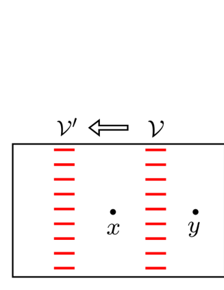
Refer to caption
Figure 9: By redefinition of variables, 𝒱𝒱\mathcal{V} is moved to 𝒱superscript𝒱\mathcal{V}^{\prime}, passing over the site x𝑥x.

Using (103) w.r.t. the hyperplane which runs through y𝑦y, with z=θ[x]𝑧𝜃delimited-[]𝑥z=\theta[x], yields

=\displaystyle=\ αG𝑑gfα(gϕx)(𝒪(g)[𝒱]T(𝟏)[𝒱])θ[fα(gϕx)(𝒪(g)[𝒱]T(𝟏)[𝒱])]1/2fα(ϕy)¯fα(ϕy)1/2subscript𝛼subscript𝐺differential-d𝑔superscriptdelimited-⟨⟩subscript𝑓𝛼𝑔subscriptitalic-ϕ𝑥𝒪𝑔delimited-[]superscript𝒱subscript𝑇1delimited-[]superscript𝒱𝜃delimited-[]subscript𝑓𝛼𝑔subscriptitalic-ϕ𝑥𝒪𝑔delimited-[]superscript𝒱subscript𝑇1delimited-[]superscript𝒱12superscriptdelimited-⟨⟩¯subscript𝑓𝛼subscriptitalic-ϕ𝑦subscript𝑓𝛼subscriptitalic-ϕ𝑦12\displaystyle\displaystyle\sum_{\alpha}\displaystyle\int_{G}dg\,\Big{\langle}f_{\alpha}(g\phi_{x})\Big{(}\mathcal{O}(g)[\mathcal{V}^{\prime}]-\mathcal{F}_{T}(\mathbf{1})[\mathcal{V}^{\prime}]\Big{)}\cdot\theta\Big{[}f_{\alpha}(g\phi_{x})\Big{(}\mathcal{O}(g)[\mathcal{V}^{\prime}]-\mathcal{F}_{T}(\mathbf{1})[\mathcal{V}^{\prime}]\Big{)}\Big{]}\Big{\rangle}^{1/2}\big{\langle}\overline{f_{\alpha}(\phi_{y})}f_{\alpha}(\phi_{y})\big{\rangle}^{1/2} (126)
=\displaystyle=\ αG𝑑gfα(gϕx)(𝒪(g)[𝒱]T(𝟏)[𝒱])fα(gϕz)¯(𝒪(g1)[𝒱θ]T(𝟏)[𝒱θ])1/2fα(ϕy)¯fα(ϕy)1/2subscript𝛼subscript𝐺differential-d𝑔superscriptdelimited-⟨⟩subscript𝑓𝛼𝑔subscriptitalic-ϕ𝑥𝒪𝑔delimited-[]superscript𝒱subscript𝑇1delimited-[]superscript𝒱¯subscript𝑓𝛼𝑔subscriptitalic-ϕ𝑧𝒪superscript𝑔1delimited-[]superscriptsuperscript𝒱𝜃subscript𝑇1delimited-[]superscriptsuperscript𝒱𝜃12superscriptdelimited-⟨⟩¯subscript𝑓𝛼subscriptitalic-ϕ𝑦subscript𝑓𝛼subscriptitalic-ϕ𝑦12\displaystyle\displaystyle\sum_{\alpha}\displaystyle\int_{G}dg\,\Big{\langle}f_{\alpha}(g\phi_{x})\Big{(}\mathcal{O}(g)[\mathcal{V}^{\prime}]-\mathcal{F}_{T}(\mathbf{1})[\mathcal{V}^{\prime}]\Big{)}\overline{f_{\alpha}(g\phi_{z})}\Big{(}\mathcal{O}(g^{-1})[{\mathcal{V}^{\prime}}^{\theta}]-\mathcal{F}_{T}(\mathbf{1})[{\mathcal{V}^{\prime}}^{\theta}]\Big{)}\Big{\rangle}^{1/2}\big{\langle}\overline{f_{\alpha}(\phi_{y})}f_{\alpha}(\phi_{y})\big{\rangle}^{1/2} (127)
=\displaystyle=\ αG𝑑gfα(gϕx)fα(gϕz)¯(1𝒪(g)[𝒱]T(𝟏)[𝒱θ]𝒪(g1)[𝒱θ]T(𝟏)[𝒱]+T(𝟏)[𝒱])1/2subscript𝛼subscript𝐺differential-d𝑔superscriptdelimited-⟨⟩subscript𝑓𝛼𝑔subscriptitalic-ϕ𝑥¯subscript𝑓𝛼𝑔subscriptitalic-ϕ𝑧1𝒪𝑔delimited-[]superscript𝒱subscript𝑇1delimited-[]superscriptsuperscript𝒱𝜃𝒪superscript𝑔1delimited-[]superscriptsuperscript𝒱𝜃subscript𝑇1delimited-[]superscript𝒱subscript𝑇1delimited-[]superscript𝒱12\displaystyle\displaystyle\sum_{\alpha}\displaystyle\int_{G}dg\,\Big{\langle}f_{\alpha}(g\phi_{x})\overline{f_{\alpha}(g\phi_{z})}\Big{(}1-\mathcal{O}(g)[\mathcal{V}^{\prime}]\mathcal{F}_{T}(\mathbf{1})[{\mathcal{V}^{\prime}}^{\theta}]-\mathcal{O}(g^{-1})[{\mathcal{V}^{\prime}}^{\theta}]\mathcal{F}_{T}(\mathbf{1})[\mathcal{V}^{\prime}]+\mathcal{F}_{T}(\mathbf{1})[\mathcal{V}^{\prime}]\Big{)}\Big{\rangle}^{1/2}
×fα(ϕy)¯fα(ϕy)1/2absentsuperscriptdelimited-⟨⟩¯subscript𝑓𝛼subscriptitalic-ϕ𝑦subscript𝑓𝛼subscriptitalic-ϕ𝑦12\displaystyle\hskip 30.0pt\times\big{\langle}\overline{f_{\alpha}(\phi_{y})}f_{\alpha}(\phi_{y})\big{\rangle}^{1/2} (128)
\displaystyle\leq\ Γμ(y;0)1/2G𝑑gΓμ(x;2n)(1𝒪(g)[𝒱]T(𝟏)[𝒱θ]𝒪(g1)[𝒱θ]T(𝟏)[𝒱]+T(𝟏)[𝒱])1/2superscriptdelimited-⟨⟩subscriptΓ𝜇𝑦012subscript𝐺differential-d𝑔superscriptdelimited-⟨⟩subscriptΓ𝜇𝑥2𝑛1𝒪𝑔delimited-[]superscript𝒱subscript𝑇1delimited-[]superscriptsuperscript𝒱𝜃𝒪superscript𝑔1delimited-[]superscriptsuperscript𝒱𝜃subscript𝑇1delimited-[]superscript𝒱subscript𝑇1delimited-[]superscript𝒱12\displaystyle\langle\Gamma_{\mu}(y;0)\rangle^{1/2}\displaystyle\int_{G}dg\,\Big{\langle}\Gamma_{\mu}(x;2n)\Big{(}1-\mathcal{O}(g)[\mathcal{V}^{\prime}]\mathcal{F}_{T}(\mathbf{1})[{\mathcal{V}^{\prime}}^{\theta}]-\mathcal{O}(g^{-1})[{\mathcal{V}^{\prime}}^{\theta}]\mathcal{F}_{T}(\mathbf{1})[\mathcal{V}^{\prime}]+\mathcal{F}_{T}(\mathbf{1})[\mathcal{V}^{\prime}]\Big{)}\Big{\rangle}^{1/2} (129)
\displaystyle\leq\ Γμ(x;0)1/2[G𝑑gΓμ(x;2n)(1𝒪(g)[𝒱]T(𝟏)[𝒱θ]𝒪(g1)[𝒱θ]T(𝟏)[𝒱]+T(𝟏)[𝒱])]1/2superscriptdelimited-⟨⟩subscriptΓ𝜇𝑥012superscriptdelimited-[]subscript𝐺differential-d𝑔delimited-⟨⟩subscriptΓ𝜇𝑥2𝑛1𝒪𝑔delimited-[]superscript𝒱subscript𝑇1delimited-[]superscriptsuperscript𝒱𝜃𝒪superscript𝑔1delimited-[]superscriptsuperscript𝒱𝜃subscript𝑇1delimited-[]superscript𝒱subscript𝑇1delimited-[]superscript𝒱12\displaystyle\langle\Gamma_{\mu}(x;0)\rangle^{1/2}\Big{[}\displaystyle\int_{G}dg\,\Big{\langle}\Gamma_{\mu}(x;2n)\Big{(}1-\mathcal{O}(g)[\mathcal{V}^{\prime}]\mathcal{F}_{T}(\mathbf{1})[{\mathcal{V}^{\prime}}^{\theta}]-\mathcal{O}(g^{-1})[{\mathcal{V}^{\prime}}^{\theta}]\mathcal{F}_{T}(\mathbf{1})[\mathcal{V}^{\prime}]+\mathcal{F}_{T}(\mathbf{1})[\mathcal{V}^{\prime}]\Big{)}\Big{\rangle}\Big{]}^{1/2} (130)
=\displaystyle=\ Γμ(x;0)1/2[Γμ(x;2n)Γμ(x;2n)T(𝟏)[𝒱]T(𝟏)[𝒱θ]Γμ(x;2n)T(𝟏)[𝒱θ]T(𝟏)[𝒱]\displaystyle\langle\Gamma_{\mu}(x;0)\rangle^{1/2}\Big{[}\langle\Gamma_{\mu}(x;2n)\rangle-\langle\Gamma_{\mu}(x;2n)\mathcal{F}_{T}(\mathbf{1})[\mathcal{V}^{\prime}]\mathcal{F}_{T}(\mathbf{1})[{\mathcal{V}^{\prime}}^{\theta}]\rangle-\langle\Gamma_{\mu}(x;2n)\mathcal{F}_{T}(\mathbf{1})[{\mathcal{V}^{\prime}}^{\theta}]\mathcal{F}_{T}(\mathbf{1})[\mathcal{V}^{\prime}]\rangle
+Γμ(x;2n)T(𝟏)[𝒱]]1/2\displaystyle\hskip 50.0pt+\langle\Gamma_{\mu}(x;2n)\mathcal{F}_{T}(\mathbf{1})[\mathcal{V}^{\prime}]\rangle\Big{]}^{1/2} (131)
=\displaystyle=\ Γμ(x;0)1/2Γμ(x;2n)(1T(𝟏)[𝒱])1/2,superscriptdelimited-⟨⟩subscriptΓ𝜇𝑥012superscriptdelimited-⟨⟩subscriptΓ𝜇𝑥2𝑛1subscript𝑇1delimited-[]superscript𝒱12\displaystyle\langle\Gamma_{\mu}(x;0)\rangle^{1/2}\langle\Gamma_{\mu}(x;2n)(1-\mathcal{F}_{T}(\mathbf{1})[\mathcal{V}^{\prime}])\rangle^{1/2}, (132)
Γμ(x;n)T(𝟏)[𝒱]Γμ(x;0){Γμ(x;2n)(1T(𝟏)[𝒱])Γμ(x;0)}1/2.thereforesuperscriptdelimited-⟨⟩subscriptΓ𝜇𝑥𝑛subscript𝑇1delimited-[]𝒱absentsubscriptdelimited-⟨⟩subscriptΓ𝜇𝑥0absentsuperscriptsuperscriptdelimited-⟨⟩subscriptΓ𝜇𝑥2𝑛1subscript𝑇1delimited-[]superscript𝒱absentsubscriptdelimited-⟨⟩subscriptΓ𝜇𝑥0absent12\therefore\ \ \displaystyle\frac{\,\langle\Gamma_{\mu}(x;n)\mathcal{F}_{T}(\mathbf{1})[\mathcal{V}]\rangle\,^{\mathstrut}}{\,\langle\Gamma_{\mu}(x;0)\rangle\,_{\mathstrut}}\leq\left\{\displaystyle\frac{\,\langle\Gamma_{\mu}(x;2n)(1-\mathcal{F}_{T}(\mathbf{1})[\mathcal{V}^{\prime}])\rangle\,^{\mathstrut}}{\,\langle\Gamma_{\mu}(x;0)\rangle\,_{\mathstrut}}\right\}^{1/2}. (133)

Combining this result with (114) yields

Γμ(x;n)T(𝟏)[𝒱]Γμ(x;0){Γμ(x;0)2Γμ(x;0)2}n/Lμ{1T(𝟏)[𝒱]}n/Lμ.superscriptdelimited-⟨⟩subscriptΓ𝜇𝑥𝑛subscript𝑇1delimited-[]𝒱absentsubscriptdelimited-⟨⟩subscriptΓ𝜇𝑥0absentsuperscriptsuperscriptdelimited-⟨⟩subscriptΓ𝜇superscript𝑥02absentsubscriptsuperscriptdelimited-⟨⟩subscriptΓ𝜇𝑥02absent𝑛subscript𝐿𝜇superscript1delimited-⟨⟩subscript𝑇1delimited-[]superscript𝒱𝑛subscript𝐿𝜇\displaystyle\frac{\,\langle\Gamma_{\mu}(x;n)\mathcal{F}_{T}(\mathbf{1})[\mathcal{V}]\rangle\,^{\mathstrut}}{\,\langle\Gamma_{\mu}(x;0)\rangle\,_{\mathstrut}}\leq\left\{\displaystyle\frac{\,\langle\Gamma_{\mu}(x;0)^{2}\rangle\,^{\mathstrut}}{\,\langle\Gamma_{\mu}(x;0)\rangle^{2}\,_{\mathstrut}}\right\}^{n/L_{\mu}}\left\{1-\langle\mathcal{F}_{T}(\mathbf{1})[\mathcal{V}^{\prime}]\rangle\right\}^{n/L_{\mu}}. (134)

(114) and (134) lead to (101). ∎

Here are a few comments:

  • 𝒪(g)delimited-⟨⟩𝒪𝑔\langle\mathcal{O}(g)\rangle is a class function on G𝐺G. It implies that when G𝐺G is a compact connected Lie group we can rewrite the integral in the r.h.s. of (101) as an integral over the maximal torus of G𝐺G with a proper Jacobian, using the Weyl’s integration formula [33].

  • According to (101), the exponential decay of the wall free energy, i.e.

    𝒪(g)[𝒱]=1O(eρ(g)Lμ)withρ(g)>0,gG,\hskip 40.0pt\langle\mathcal{O}(g)[\mathcal{V}]\rangle=1-O({\mathrm{e}}^{-\rho(g)L_{\mu}}){\hskip 20.0pt\rm{with}\ \ }\rho(g)>0,\ \ \ ^{\forall}g\in G, (135)

    is a sufficient condition for the existence of a mass gap. Indeed if we define ρ¯[G]mingGρ(g)¯𝜌delimited-[]𝐺subscript𝑔𝐺𝜌𝑔\overline{\rho}[G]\equiv\displaystyle\min_{g\in G}\,\rho(g) and take the limit Lμsubscript𝐿𝜇L_{\mu}\to\infty, the r.h.s. of (101) converges to O(1)×eρ¯[G]n𝑂1superscripte¯𝜌delimited-[]𝐺𝑛O(1)\times{\mathrm{e}}^{-\overline{\rho}[G]n}, thus ρ¯[G]¯𝜌delimited-[]𝐺\overline{\rho}[G] gives a lower bound for the mass gap. It is also obvious that ρ¯[G]ρ¯[H]¯𝜌delimited-[]𝐺¯𝜌delimited-[]𝐻\overline{\rho}[G]\leq\overline{\rho}[H] follows if HG𝐻𝐺H\subset G. 𝒪(g)[𝒱]delimited-⟨⟩𝒪𝑔delimited-[]𝒱\langle\mathcal{O}(g)[\mathcal{V}]\rangle would be calculable by, for example, Monte Carlo Simulations and weak-coupling-, strong-coupling-, 1/d1𝑑1/d- and 1/N1𝑁1/N-expansions.

  • We proved the theorem on a square lattice, but it can be easily generalized to other lattices such as a triangular lattice.

  • Note that theorem 5 is derived with no knowledge of the interaction except for the reflection positivity. The strength of interaction can be made anisotropic, since it respects reflection positivity. And it is also correct in arbitrary dimensions.

3.3 Examples

There are many classes of lattice systems to which our theorem is applicable. One is the class of coset models, where the field takes values in G/H𝐺𝐻G/H with G𝐺G an arbitrary Lie group and H𝐻H its closed subgroup. We present three explicit examples.

Example 1.

The O(N)𝑂𝑁O(N) Heisenberg model.

The partition function is given by

Z=yΛdϕyexp(βx,μϕxϕx+μ^),ϕSN1=O(N)/O(N1).formulae-sequence𝑍subscriptproduct𝑦Λ𝑑subscriptitalic-ϕ𝑦𝛽subscript𝑥𝜇subscriptitalic-ϕ𝑥subscriptitalic-ϕ𝑥^𝜇italic-ϕsuperscript𝑆𝑁1𝑂𝑁𝑂𝑁1\hskip 60.0ptZ=\displaystyle\int\prod_{y\in\Lambda}d\vec{\phi}_{y}\ \exp\Big{(}\beta\displaystyle\sum_{x,\mu}\vec{\phi}_{x}\cdot\vec{\phi}_{x+\hat{\mu}}\Big{)},\hskip 20.0pt\vec{\phi}\in S^{N-1}=O(N)/O(N-1). (136)

The most natural definition of a correlation function is

Γμ(x;n)=ϕxϕx+nμ^.subscriptΓ𝜇𝑥𝑛subscriptitalic-ϕ𝑥subscriptitalic-ϕ𝑥𝑛^𝜇\Gamma_{\mu}(x;n)=\vec{\phi}_{x}\cdot\vec{\phi}_{x+n\hat{\mu}}. (137)

In this case Z2subscript𝑍2Z_{2} is obviously the smallest possible invariance group; of course, O(N)𝑂𝑁O(N) itself can also be chosen. One can check that the requirements (99), (100) are met for both of them. If one is going to choose other arbitrary subgroup of O(N)𝑂𝑁O(N), the correlation function should be redefined properly as explained below (100). Since the length of spin is normalized, the prefactor in (101) becomes 1.

Example 2.

The CPN1𝐶superscript𝑃𝑁1CP^{N-1} model.

The partition function is given by161616See also ref.[34].

Z=yΛdPyexp(βx,μTr[PxPx+μ^]),PCPN1=U(N)/(U(1)×U(N1)).formulae-sequence𝑍subscriptproduct𝑦Λ𝑑subscript𝑃𝑦𝛽subscript𝑥𝜇Trdelimited-[]subscript𝑃𝑥subscript𝑃𝑥^𝜇𝑃𝐶superscript𝑃𝑁1𝑈𝑁𝑈1𝑈𝑁1Z=\displaystyle\int\prod_{y\in\Lambda}dP_{y}\ \exp\Big{(}\beta\displaystyle\sum_{x,\mu}\mathrm{Tr}\,[P_{x}P_{x+\hat{\mu}}]\Big{)},\hskip 20.0ptP\in CP^{N-1}=U(N)/(U(1)\times U(N-1)). (138)

P𝑃P is an N×N𝑁𝑁N\times N matrix and obeys Px2=Px,Px=Px,TrPx=1formulae-sequencesuperscriptsubscript𝑃𝑥2subscript𝑃𝑥formulae-sequencesuperscriptsubscript𝑃𝑥subscript𝑃𝑥Trsubscript𝑃𝑥1P_{x}^{2}=P_{x},\ P_{x}^{\dagger}=P_{x},\ \mathrm{Tr}\,P_{x}=1. (An alternative way is to express Pij=zizjsubscript𝑃𝑖𝑗superscriptsubscript𝑧𝑖subscript𝑧𝑗P_{ij}=z_{i}^{*}z_{j}, where zN𝑧superscript𝑁\vec{z}\in\mathbb{C}^{N} and |z|2=1superscript𝑧21|\vec{z}|^{2}=1.) The action is invariant under the global transformation PxΩPxΩsubscript𝑃𝑥Ωsubscript𝑃𝑥superscriptΩP_{x}\to\Omega P_{x}\Omega^{\dagger} with ΩSU(N)Ω𝑆𝑈𝑁\Omega\in SU(N).171717The true symmetry is SU(N)/ZN𝑆𝑈𝑁subscript𝑍𝑁SU(N)/Z_{N}, since ΩZNΩsubscript𝑍𝑁\Omega\in Z_{N} does not change Pxsubscript𝑃𝑥P_{x} at all. In two dimension, the model is believed to possess a nonperturbatively generated mass gap for which, however, no rigorous result is available. Defining an appropriate correlation function needs some care; we define

Γμ(x;n)=Tr{[Px 1NN][Px+nμ^ 1NN]}=Tr[PxPx+nμ^] 1N,subscriptΓ𝜇𝑥𝑛Trdelimited-[]subscript𝑃𝑥superscriptsubscript1𝑁absentsubscript𝑁absentdelimited-[]subscript𝑃𝑥𝑛^𝜇superscriptsubscript1𝑁absentsubscript𝑁absentTrdelimited-[]subscript𝑃𝑥subscript𝑃𝑥𝑛^𝜇superscript1absentsubscript𝑁absent\Gamma_{\mu}(x;n)=\mathrm{Tr\,}\left\{[P_{x}-\displaystyle\frac{\,\mathbf{1}_{N}\,^{\mathstrut}}{\,N\,_{\mathstrut}}][P_{x+n\hat{\mu}}-\displaystyle\frac{\,\mathbf{1}_{N}\,^{\mathstrut}}{\,N\,_{\mathstrut}}]\right\}=\mathrm{Tr\,}[P_{x}P_{x+n\hat{\mu}}]-\displaystyle\frac{\,1\,^{\mathstrut}}{\,N\,_{\mathstrut}}, (139)

where 𝟏Nsubscript1𝑁\mathbf{1}_{N} denotes the unit matrix of size N×N𝑁𝑁N\times N. Then it is easy to confirm (100) for G=SU(N)𝐺𝑆𝑈𝑁G=SU(N):

SU(N)𝑑Ω[ΩPΩ 1NN]ijsubscript𝑆𝑈𝑁differential-dΩsubscriptdelimited-[]Ω𝑃superscriptΩsuperscriptsubscript1𝑁absentsubscript𝑁absent𝑖𝑗\displaystyle\displaystyle\int_{SU(N)}d\Omega\,\Big{[}\Omega P\Omega^{\dagger}-\displaystyle\frac{\,\mathbf{1}_{N}\,^{\mathstrut}}{\,N\,_{\mathstrut}}\Big{]}_{ij} =PklSU(N)𝑑ΩΩikΩljδijNabsentsubscript𝑃𝑘𝑙subscript𝑆𝑈𝑁differential-dΩsubscriptΩ𝑖𝑘subscriptsuperscriptΩ𝑙𝑗superscriptsubscript𝛿𝑖𝑗absentsubscript𝑁absent\displaystyle=P_{kl}\displaystyle\int_{SU(N)}d\Omega\ \Omega_{ik}{\Omega^{\dagger}}_{lj}-\displaystyle\frac{\,\delta_{ij}\,^{\mathstrut}}{\,N\,_{\mathstrut}} (140)
=PklδijδklNδijN=0.absentsubscript𝑃𝑘𝑙subscript𝛿𝑖𝑗superscriptsubscript𝛿𝑘𝑙absentsubscript𝑁absentsuperscriptsubscript𝛿𝑖𝑗absentsubscript𝑁absent0\displaystyle=P_{kl}\displaystyle\frac{\,\delta_{ij}\delta_{kl}\,^{\mathstrut}}{\,N\,_{\mathstrut}}-\displaystyle\frac{\,\delta_{ij}\,^{\mathstrut}}{\,N\,_{\mathstrut}}=0. (141)
Example 3.

G×G𝐺𝐺G\times G principal chiral model (PCM).

Here G𝐺G is an arbitrary compact group. The partition function is given by

Z=yΛdUyexp(βx,μΛReTr[Ux(Ux+μ^)1]),UxG.formulae-sequence𝑍subscriptproduct𝑦Λ𝑑subscript𝑈𝑦𝛽subscript𝑥𝜇ΛReTrdelimited-[]subscript𝑈𝑥superscriptsubscript𝑈𝑥^𝜇1subscript𝑈𝑥𝐺Z=\displaystyle\int\prod_{y\in\Lambda}dU_{y}\ \exp\left(\beta\displaystyle\sum_{x,\mu\subset\Lambda}{\mathrm{Re\,Tr\,}}[U_{x}(U_{x+\hat{\mu}})^{-1}]\right),\hskip 20.0ptU_{x}\in G. (142)

This model is invariant under a global G×G𝐺𝐺G\times G transformation UgLUgR1𝑈subscript𝑔𝐿𝑈superscriptsubscript𝑔𝑅1U\to g_{L}Ug_{R}^{-1}. The corresponding twisted partition function is given, in agreement with the original definition (62), by (𝒱𝒱\mathcal{V} : wall)

Z(g)=yΛdUyexp(βx,μΛ𝒱ReTr[Ux(Ux+μ^)1]+βx,μ𝒱ReTr[Ux(gUx+μ^)1]),gG.formulae-sequence𝑍𝑔subscriptproduct𝑦Λ𝑑subscript𝑈𝑦𝛽subscript𝑥𝜇Λ𝒱ReTrdelimited-[]subscript𝑈𝑥superscriptsubscript𝑈𝑥^𝜇1𝛽subscript𝑥𝜇𝒱ReTrdelimited-[]subscript𝑈𝑥superscript𝑔subscript𝑈𝑥^𝜇1𝑔𝐺Z(g)=\displaystyle\int\prod_{y\in\Lambda}dU_{y}\ \exp\left(\beta\displaystyle\sum_{x,\mu\subset\Lambda\setminus\mathcal{V}}{\mathrm{Re\,Tr\,}}[U_{x}(U_{x+\hat{\mu}})^{-1}]+\beta\displaystyle\sum_{x,\mu\subset\mathcal{V}}{\mathrm{Re\,Tr\,}}[U_{x}(gU_{x+\hat{\mu}})^{-1}]\right),\hskip 20.0ptg\in G. (143)

The correlation function is defined as

Γμ(x;n)=χR(UxUx+nμ^1),subscriptΓ𝜇𝑥𝑛subscript𝜒𝑅subscript𝑈𝑥subscriptsuperscript𝑈1𝑥𝑛^𝜇\Gamma_{\mu}(x;n)=\chi_{R}(U_{x}U^{-1}_{x+n\hat{\mu}}), (144)

where R𝑅R denotes an irreducible unitary representation of G𝐺G. If we choose G𝐺G itself, then (100) is satisfied if and only if R𝑅R is a nontrivial representation. This is a direct consequence of the Schur orthogonality relation in representation theory; see Corollary 4.10 in ref.[33]. If G=SU(N)𝐺𝑆𝑈𝑁G=SU(N) and we choose ZNsubscript𝑍𝑁Z_{N}, then (100) is satisfied iff R𝑅R has a nonzero N𝑁N-ality. Anyway the prefactor in (101) becomes 1. We emphasize that G𝐺G need not have a nontrivial center.

As an example other than coset models, we only present

Example 4.

SU(Nf)×SU(Nf)𝑆𝑈subscript𝑁𝑓𝑆𝑈subscript𝑁𝑓SU(N_{f})\times SU(N_{f}) linear sigma model.

Usually this model is used to study the chiral phase transition [35]. On the lattice, the partition function is given by

Z=yΛdΦyexp(β1x,μReTr(ΦxΦx+μ^)β2xΛTr(ΦxΦx)λ1xΛ[Tr(ΦxΦx)]2λ2xΛTr(ΦxΦx)2),𝑍subscriptproduct𝑦Λ𝑑subscriptΦ𝑦subscript𝛽1subscript𝑥𝜇ReTrsubscriptΦ𝑥subscriptsuperscriptΦ𝑥^𝜇subscript𝛽2subscript𝑥ΛTrsuperscriptsubscriptΦ𝑥subscriptΦ𝑥subscript𝜆1subscript𝑥Λsuperscriptdelimited-[]TrsuperscriptsubscriptΦ𝑥subscriptΦ𝑥2subscript𝜆2subscript𝑥ΛTrsuperscriptsuperscriptsubscriptΦ𝑥subscriptΦ𝑥2\displaystyle Z=\displaystyle\int\prod_{y\in\Lambda}d\Phi_{y}\ \exp\Big{(}\beta_{1}\displaystyle\sum_{x,\mu}{\mathrm{Re\,Tr\,}}(\Phi_{x}\Phi^{\dagger}_{x+\hat{\mu}})-\beta_{2}\displaystyle\sum_{x\in\Lambda}{\mathrm{Tr\,}}(\Phi_{x}^{\dagger}\Phi_{x})-\lambda_{1}\displaystyle\sum_{x\in\Lambda}\big{[}{\mathrm{Tr\,}}(\Phi_{x}^{\dagger}\Phi_{x})\big{]}^{2}-\lambda_{2}\displaystyle\sum_{x\in\Lambda}{\mathrm{Tr\,}}(\Phi_{x}^{\dagger}\Phi_{x})^{2}\Big{)}, (145)
ΦxM(Nf,).subscriptΦ𝑥Msubscript𝑁𝑓\displaystyle\hskip 20.0pt\Phi_{x}\in{\mathrm{M}}(N_{f},\mathbb{C}). (146)

This model is invariant under ΦeiαgLΦgRΦsuperscripte𝑖𝛼subscript𝑔𝐿Φsubscriptsuperscript𝑔𝑅\Phi\to{\mathrm{e}}^{i\alpha}g_{L}\Phi g^{\dagger}_{R} with eiαUA(1)superscripte𝑖𝛼subscript𝑈𝐴1{\mathrm{e}}^{i\alpha}\in U_{A}(1) and gL,gRSU(Nf)subscript𝑔𝐿subscript𝑔𝑅𝑆𝑈subscript𝑁𝑓g_{L},g_{R}\in SU(N_{f}).

It might be the case that whether the upper bound (101) gives an exponential decay or not depends on the choice of G𝐺G, a point worth further study.
                        *                        *                        *                        *

Although we proved theorem 5 only in the case of the nearest-neighbor interaction, we can prove it even in the presence of non-nearest-neighbor and multi-site interactions if some appropriate conditions are satisfied. To make the argument concrete, let us consider the SU(N)×SU(N)𝑆𝑈𝑁𝑆𝑈𝑁SU(N)\times SU(N) PCM and suppose that ZNSU(N)subscript𝑍𝑁𝑆𝑈𝑁Z_{N}\subset SU(N) was chosen as a symmetry group for theorem 5. There are two crucial conditions: one is site-reflection positivity and the other is that twists and their algebra (see 3.1) should remain well-defined. Here is a partial list of possible extensions (on a square lattice):

  1. 1.

    The multi-site interaction term between four variables on the same plaquette,

    ReχR(UxUx+μ^Ux+μ^+ν^Ux+ν^),Resubscript𝜒𝑅subscript𝑈𝑥subscriptsuperscript𝑈𝑥^𝜇subscript𝑈𝑥^𝜇^𝜈subscriptsuperscript𝑈𝑥^𝜈\mathrm{Re\,}\chi_{R}(U_{x}U^{\dagger}_{x+\hat{\mu}}U_{x+\hat{\mu}+\hat{\nu}}U^{\dagger}_{x+\hat{\nu}}), (147)

    can be added to the action without spoiling theorem 5 if the N𝑁N-ality of R𝑅R is 0.

  2. 2.

    The non-nearest-neighbor interaction term ReχR(UxUx+2μ^)Resubscript𝜒𝑅subscript𝑈𝑥subscriptsuperscript𝑈𝑥2^𝜇\mathrm{Re\,}\chi_{R}(U_{x}U^{\dagger}_{x+2\hat{\mu}}) can be added to the action if the N𝑁N-ality of R𝑅R is 0 and the coefficient in front of it is positive. (If the distance is larger than two lattice spacings, or if the coefficient is negative, then the site-reflection positivity becomes hard to prove.)

  3. 3.

    The non-nearest-neighbor interaction term ReχR(UxUx+μ^+ν^)Resubscript𝜒𝑅subscript𝑈𝑥subscriptsuperscript𝑈𝑥^𝜇^𝜈\mathrm{Re\,}\chi_{R}(U_{x}U^{\dagger}_{x+\hat{\mu}+\hat{\nu}}), μν𝜇𝜈\mu\neq\nu, can be added to the action if the N𝑁N-ality of R𝑅R is 0.

*                        *                        *                        *

Note that our proved inequality may fail to be useful in phases other than the disordered phase, even though it is correct in any phases. Consider a spin system with a global symmetry group G𝐺G in a d𝑑d-dimensional box of size L1××Ldsubscript𝐿1subscript𝐿𝑑L_{1}\times\dots\times L_{d} whose boundary condition is twisted by gG𝑔𝐺g\in G in the x1superscript𝑥1x^{1}-direction and otherwise periodic. Let Zgsuperscript𝑍𝑔Z^{g} denote the twisted partition function and set Lk=2dLksubscript𝐿perpendicular-tosuperscriptsubscriptproduct𝑘2𝑑subscript𝐿𝑘\displaystyle L_{\perp}\equiv\prod_{k=2}^{d}L_{k}. Based on our experience in gauge theories, we generally expect following behaviors of Zg/Zsuperscript𝑍𝑔𝑍Z^{g}/Z in various phases:

Zg/Zexp(xLexp(yL1))(Disordered phase)Zg/Zexp(zL)(Ordered phase)Zg/Zexp(wL/L1)(Massless phase)superscript𝑍𝑔𝑍𝑥subscript𝐿perpendicular-to𝑦subscript𝐿1(Disordered phase)superscript𝑍𝑔𝑍𝑧subscript𝐿perpendicular-to(Ordered phase)superscript𝑍𝑔𝑍𝑤subscript𝐿perpendicular-tosubscript𝐿1(Massless phase)\begin{array}[]{lr}Z^{g}/Z\approx\exp(-xL_{\perp}\exp(-yL_{1}))&\textrm{(Disordered phase)}\\ Z^{g}/Z\approx\exp(-zL_{\perp})&\textrm{(Ordered phase)}\\ Z^{g}/Z\approx\exp(-wL_{\perp}/L_{1})&\textrm{(Massless phase)}\end{array} (148)

where x,y,z𝑥𝑦𝑧x,y,z and w𝑤w are functions of the coupling constants and the choice of g𝑔g. Letting α𝛼\alpha denote the value of (1Zg/Z)1/L1superscript1superscript𝑍𝑔𝑍1subscript𝐿1(1-Z^{g}/Z)^{1/L_{1}} in the thermodynamic limit, we have α=ey𝛼superscripte𝑦\alpha={\mathrm{e}}^{-y} in the disordered phase, while α=1𝛼1\alpha=1 in the other cases so that the r.h.s. of (101) tends to a constant independent of n𝑛n. So the bottom line is that algebraic decay of correlation function cannot be inferred from the behavior of the r.h.s. in general.

Finally we comment on the formal difference between the inequality derived by Kova´csKov´acs{\rm{Kov\acute{a}cs}} and Tomboulis in refs.[19, 20] and ours in the two-dimensional SU(2)×SU(2)𝑆𝑈2𝑆𝑈2SU(2)\times SU(2) PCM. Their result is

Γμ(x;n)|Lμ=Zn(+,+)Zn(,)Zn(+,+)+Zn(+,)+Zn(,+)+Zn(,),evaluated-atdelimited-⟨⟩subscriptΓ𝜇𝑥𝑛subscript𝐿𝜇subscript𝑍𝑛subscript𝑍𝑛superscriptabsentsubscript𝑍𝑛subscript𝑍𝑛subscript𝑍𝑛subscript𝑍𝑛subscriptabsent\langle\Gamma_{\mu}(x;n)\rangle\Big{|}_{L_{\mu}=\infty}\leq\displaystyle\frac{\,Z_{n}(+,+)-Z_{n}(-,-)\,^{\mathstrut}}{\,Z_{n}(+,+)+Z_{n}(+,-)+Z_{n}(-,+)+Z_{n}(-,-)\,_{\mathstrut}}, (149)

where Zn(τ1,τ2)(τ1,2=±1)subscript𝑍𝑛subscript𝜏1subscript𝜏2subscript𝜏12plus-or-minus1Z_{n}(\tau_{1},\tau_{2})\ (\tau_{1,2}=\pm 1) is the partition function on the lattice of size n×n𝑛𝑛n\times n with a twist τμsubscript𝜏𝜇\tau_{\mu} operated in the xμsuperscript𝑥𝜇x^{\mu}-direction.

On the other hand, our result ((101) with G=Z2𝐺subscript𝑍2G=Z_{2}) gives

Γμ(x;n)delimited-⟨⟩subscriptΓ𝜇𝑥𝑛\displaystyle\langle\Gamma_{\mu}(x;n)\rangle 2{10[𝒱]}n/Lμabsent2superscript1delimited-⟨⟩subscript0delimited-[]𝒱𝑛subscript𝐿𝜇\displaystyle\leq 2\left\{1-\langle\mathcal{F}_{0}[\mathcal{V}]\rangle\right\}^{n/L_{\mu}} (150)
=2{ 1 2[ZLμ(+,+)ZLμ(+,)ZLμ(+,+)]}n/Lμ.absent2superscriptsuperscript1absentsubscript2absentdelimited-[]subscript𝑍subscript𝐿𝜇subscript𝑍subscript𝐿𝜇superscriptabsentsubscript𝑍subscript𝐿𝜇subscriptabsent𝑛subscript𝐿𝜇\displaystyle=2\left\{\displaystyle\frac{\,1\,^{\mathstrut}}{\,2\,_{\mathstrut}}\Bigg{[}\displaystyle\frac{\,Z_{L_{\mu}}(+,+)-Z_{L_{\mu}}(+,-)\,^{\mathstrut}}{\,Z_{L_{\mu}}(+,+)\,_{\mathstrut}}\Bigg{]}\right\}^{n/L_{\mu}}. (151)

Note that in the latter, both r.h.s. and l.h.s. are estimated on the lattice of size Lμsubscript𝐿𝜇L_{\mu}. In both formulas the correlation function is assumed to be in the fundamental representation. Although they look different, both relates the exponential suppression of the wall free energy (in the thermodynamic limit) to the mass gap, thus their physical contents are totally consistent.

3.4 Demonstration in 1D PCM and 2D square Ising model

Let us verify the proved inequality (101) explicitly in the G×G𝐺𝐺G\times G PCM in one-dimension, with G𝐺G an arbitrary compact group. The partition function of the model on a periodic chain of length L𝐿L is given by

ZΛsubscript𝑍Λ\displaystyle Z_{\Lambda} k=1LdUkexp(βi=1LReTr(UiUi+11)),β>0,UiG,formulae-sequenceabsentsuperscriptsubscriptproduct𝑘1𝐿𝑑subscript𝑈𝑘𝛽superscriptsubscript𝑖1𝐿ReTrsubscript𝑈𝑖superscriptsubscript𝑈𝑖11formulae-sequence𝛽0subscript𝑈𝑖𝐺\displaystyle\equiv\int\prod_{k=1}^{L}dU_{k}\ \exp\Big{(}\beta\displaystyle\sum_{i=1}^{L}{\mathrm{Re\ Tr\ }}(U_{i}U_{i+1}^{-1})\Big{)},\hskip 40.0pt\beta>0,\ U_{i}\in G, (152)
=k=1LdUki=1L[rdrFrχr(UiUi+11)],absentsuperscriptsubscriptproduct𝑘1𝐿𝑑subscript𝑈𝑘superscriptsubscriptproduct𝑖1𝐿delimited-[]subscript𝑟subscript𝑑𝑟subscript𝐹𝑟subscript𝜒𝑟subscript𝑈𝑖superscriptsubscript𝑈𝑖11\displaystyle=\int\prod_{k=1}^{L}dU_{k}\ \prod_{i=1}^{L}\Big{[}\displaystyle\sum_{r}d_{r}F_{r}\chi_{r}(U_{i}U_{i+1}^{-1})\Big{]}, (153)

where rsubscript𝑟\displaystyle\sum_{r} runs over all irreducible unitary representations of G𝐺G. Fr=Fr¯>0subscript𝐹𝑟subscript𝐹¯𝑟0F_{r}=F_{\overline{r}}>0 follows from the reflection positivity and reality of the action. Let us define crFr/F0subscript𝑐𝑟subscript𝐹𝑟subscript𝐹0c_{r}\equiv F_{r}/F_{0} for later convenience (00 denotes the trivial representation). Straightforward calculation yields

ZΛ=rdr2(Fr)L.subscript𝑍Λsubscript𝑟superscriptsubscript𝑑𝑟2superscriptsubscript𝐹𝑟𝐿Z_{\Lambda}=\displaystyle\sum_{r}d_{r}^{2}(F_{r})^{L}. (154)

The twisted partition function ZΛgsuperscriptsubscript𝑍Λ𝑔Z_{\Lambda}^{g} is similarly given by

ZΛgsuperscriptsubscript𝑍Λ𝑔\displaystyle Z_{\Lambda}^{g} k=1LdUk[rdrFrχr(gU1U21)]i=2L[rdrFrχr(UiUi+11)],gG,formulae-sequenceabsentsuperscriptsubscriptproduct𝑘1𝐿𝑑subscript𝑈𝑘delimited-[]subscriptsuperscript𝑟subscript𝑑superscript𝑟subscript𝐹superscript𝑟subscript𝜒superscript𝑟𝑔subscript𝑈1superscriptsubscript𝑈21superscriptsubscriptproduct𝑖2𝐿delimited-[]subscript𝑟subscript𝑑𝑟subscript𝐹𝑟subscript𝜒𝑟subscript𝑈𝑖superscriptsubscript𝑈𝑖11𝑔superscript𝐺\displaystyle\equiv\int\prod_{k=1}^{L}dU_{k}\ \Big{[}\displaystyle\sum_{r^{\prime}}d_{r^{\prime}}F_{r^{\prime}}\chi_{r^{\prime}}(gU_{1}U_{2}^{-1})\Big{]}\prod_{i=2}^{L}\Big{[}\displaystyle\sum_{r}d_{r}F_{r}\chi_{r}(U_{i}U_{i+1}^{-1})\Big{]},\hskip 40.0ptg\in G^{\prime}, (155)
=rdrχr(g)(Fr)L,absentsubscript𝑟subscript𝑑𝑟subscript𝜒𝑟𝑔superscriptsubscript𝐹𝑟𝐿\displaystyle=\displaystyle\sum_{r}d_{r}\chi_{r}(g)(F_{r})^{L}, (156)

where GGsuperscript𝐺𝐺G^{\prime}\subset G is an arbitrary subgroup of G𝐺G. (ZΛgsuperscriptsubscript𝑍Λ𝑔Z_{\Lambda}^{g} reduces to ZΛsubscript𝑍ΛZ_{\Lambda} for g=𝟏𝑔1g=\mathbf{1}, as it should be.) Hence we get

limL{1G𝑑g𝒪(g)}n/Lsubscript𝐿superscript1subscriptsuperscript𝐺differential-d𝑔delimited-⟨⟩𝒪𝑔𝑛𝐿\displaystyle\displaystyle\lim_{L\to\infty}\Big{\{}1-\int_{G^{\prime}}dg\langle\mathcal{O}(g)\rangle\Big{\}}^{n/L} =limL{rdr2(cr)Lrdr2(cr)L}n/L\displaystyle=\displaystyle\lim_{L\to\infty}\left\{\displaystyle\frac{\,{\displaystyle\sum_{r}}^{\prime}d_{r}^{2}(c_{r})^{L}\,{}^{\mathstrut}}{\,\displaystyle\sum_{r}d_{r}^{2}(c_{r})^{L}\,_{\mathstrut}}\right\}^{n/L} (157)
=(cr)n.absentsuperscriptsubscript𝑐superscript𝑟𝑛\displaystyle=(c_{r^{\prime}})^{n}. (158)

Here rsuperscriptsubscript𝑟{\displaystyle\sum_{r}}^{\prime} is defined as a sum over all representations of G𝐺G which are nontrivial w.r.t. Gsuperscript𝐺G^{\prime}, and crsubscript𝑐superscript𝑟c_{r^{\prime}} is defined as the largest one among {cr|ris nontrivial w.r.t. G}conditional-setsubscript𝑐𝑟𝑟is nontrivial w.r.t. superscript𝐺\{c_{r}\ |\ r\ {\textrm{is\ nontrivial\ w.r.t.\ }G^{\prime}}\}.

Next we define the correlation function as Γ(n)=χR(U0Un1)Γ𝑛subscript𝜒𝑅subscript𝑈0superscriptsubscript𝑈𝑛1\Gamma(n)=\chi_{R}(U_{0}U_{n}^{-1}). Then (100) requires R𝑅R to be nontrivial w.r.t. G𝐺G. After straightforward calculation we get

Γ(n)Γ(0)= 1dRχR(U0Un1)=(cR)n\displaystyle\frac{\,\langle\Gamma(n)\rangle\,^{\mathstrut}}{\,\langle\Gamma(0)\rangle\,_{\mathstrut}}=\displaystyle\frac{\,1\,^{\mathstrut}}{\,d_{R}\,{}_{\mathstrut}}\langle\chi_{R}(U_{0}U_{n}^{-1})\rangle=(c_{R})^{n} (159)

in the thermodynamic limit (L𝐿L\to\infty). Since cRcrsubscript𝑐𝑅subscript𝑐superscript𝑟c_{R}\leq c_{r^{\prime}} is obvious from their definitions, we conclude from (158) and (159) that the inequality (101) certainly holds at least in the limit L𝐿L\to\infty. 181818(101) should hold for finite L𝐿L too, but expressions of both sides of (101) become highly complicated for finite L𝐿L and verification seems to be hard.
                        *                        *                        *                        *

As a next example let us take the two-dimensional Ising model on a square lattice. The partition function of the model is given by

ZΛ=kΛdσkexp(μ=1L1ν=1L2(aσμνσμ+1,ν+bσμνσμ,ν+1)),subscript𝑍Λsubscriptproduct𝑘Λ𝑑subscript𝜎𝑘superscriptsubscript𝜇1subscript𝐿1superscriptsubscript𝜈1subscript𝐿2𝑎subscript𝜎𝜇𝜈subscript𝜎𝜇1𝜈𝑏subscript𝜎𝜇𝜈subscript𝜎𝜇𝜈1Z_{\Lambda}=\int\prod_{k\in\Lambda}d\sigma_{k}\ \exp\left(\displaystyle\sum_{\mu=1}^{L_{1}}\displaystyle\sum_{\nu=1}^{L_{2}}(a\sigma_{\mu\nu}\sigma_{\mu+1,\nu}+b\sigma_{\mu\nu}\sigma_{\mu,\nu+1})\right), (160)

where σμνsubscript𝜎𝜇𝜈\sigma_{\mu\nu} is the Ising spin located at the site (μ,ν)𝜇𝜈(\mu,\nu) and 𝑑σ 1 2σ=±1differential-d𝜎superscript1absentsubscript2absentsubscript𝜎plus-or-minus1\displaystyle\int d\sigma\equiv\displaystyle\frac{\,1\,^{\mathstrut}}{\,2\,_{\mathstrut}}\displaystyle\sum_{\sigma=\pm 1}. Periodic boundary conditions are imposed so that σ1,ν=σL1+1,ν,σμ,1=σμ,L2+1formulae-sequencesubscript𝜎1𝜈subscript𝜎subscript𝐿11𝜈subscript𝜎𝜇1subscript𝜎𝜇subscript𝐿21\sigma_{1,\nu}=\sigma_{L_{1}+1,\nu},\,\sigma_{\mu,1}=\sigma_{\mu,L_{2}+1}. We assume a>0,b>0formulae-sequence𝑎0𝑏0a>0,\,b>0. Let us focus on the high temperature (disorder) phase of the model.

The exact asymptotic form of the two-point correlation function is known [36] and the mass gap (or inverse correlation length) M2(a¯b)𝑀2¯𝑎𝑏M\equiv 2(\overline{a}-b), where a¯¯𝑎\overline{a} is the dual temperature defined by

sinh2asinh2a¯=1.2𝑎2¯𝑎1\sinh 2a\ \sinh 2\overline{a}=1. (161)

b¯¯𝑏\overline{b} is defined in the same way.

To estimate the free energy of walls we need explicit formulae for twisted and untwisted partition functions. Here we use the expressions due to Kastening [37], which in out notation read

ZΛ= 1 2[2sinh(2a)]L1L2/2×\displaystyle Z_{\Lambda}=\displaystyle\frac{\,1\,^{\mathstrut}}{\,2\,_{\mathstrut}}[2\sinh(2a)]^{L_{1}L_{2}/2}\times
{k=1L2[2cosh(L1 2γ2k1)]+k=1L2[2sinh(L1 2γ2k1)]+k=1L2[2cosh(L1 2γ2k2)]k=1L2[2sinh(L1 2γ2k2)]},superscriptsubscriptproduct𝑘1subscript𝐿2delimited-[]2superscriptsubscript𝐿1absentsubscript2absentsubscript𝛾2𝑘1superscriptsubscriptproduct𝑘1subscript𝐿2delimited-[]2superscriptsubscript𝐿1absentsubscript2absentsubscript𝛾2𝑘1superscriptsubscriptproduct𝑘1subscript𝐿2delimited-[]2superscriptsubscript𝐿1absentsubscript2absentsubscript𝛾2𝑘2superscriptsubscriptproduct𝑘1subscript𝐿2delimited-[]2superscriptsubscript𝐿1absentsubscript2absentsubscript𝛾2𝑘2\displaystyle\left\{\prod_{k=1}^{L_{2}}\Big{[}2\cosh\Big{(}\displaystyle\frac{\,L_{1}\,^{\mathstrut}}{\,2\,_{\mathstrut}}\gamma_{2k-1}\Big{)}\Big{]}+\prod_{k=1}^{L_{2}}\Big{[}2\sinh\Big{(}\displaystyle\frac{\,L_{1}\,^{\mathstrut}}{\,2\,_{\mathstrut}}\gamma_{2k-1}\Big{)}\Big{]}+\prod_{k=1}^{L_{2}}\Big{[}2\cosh\Big{(}\displaystyle\frac{\,L_{1}\,^{\mathstrut}}{\,2\,_{\mathstrut}}\gamma_{2k-2}\Big{)}\Big{]}-\prod_{k=1}^{L_{2}}\Big{[}2\sinh\Big{(}\displaystyle\frac{\,L_{1}\,^{\mathstrut}}{\,2\,_{\mathstrut}}\gamma_{2k-2}\Big{)}\Big{]}\right\}, (162)
ZΛ()= 1 2[2sinh(2a)]L1L2/2×\displaystyle Z_{\Lambda}^{(-)}=\displaystyle\frac{\,1\,^{\mathstrut}}{\,2\,_{\mathstrut}}[2\sinh(2a)]^{L_{1}L_{2}/2}\times
{k=1L2[2cosh(L1 2γ2k1)]+k=1L2[2sinh(L1 2γ2k1)]k=1L2[2cosh(L1 2γ2k2)]+k=1L2[2sinh(L1 2γ2k2)]}.superscriptsubscriptproduct𝑘1subscript𝐿2delimited-[]2superscriptsubscript𝐿1absentsubscript2absentsubscript𝛾2𝑘1superscriptsubscriptproduct𝑘1subscript𝐿2delimited-[]2superscriptsubscript𝐿1absentsubscript2absentsubscript𝛾2𝑘1superscriptsubscriptproduct𝑘1subscript𝐿2delimited-[]2superscriptsubscript𝐿1absentsubscript2absentsubscript𝛾2𝑘2superscriptsubscriptproduct𝑘1subscript𝐿2delimited-[]2superscriptsubscript𝐿1absentsubscript2absentsubscript𝛾2𝑘2\displaystyle\left\{\prod_{k=1}^{L_{2}}\Big{[}2\cosh\Big{(}\displaystyle\frac{\,L_{1}\,^{\mathstrut}}{\,2\,_{\mathstrut}}\gamma_{2k-1}\Big{)}\Big{]}+\prod_{k=1}^{L_{2}}\Big{[}2\sinh\Big{(}\displaystyle\frac{\,L_{1}\,^{\mathstrut}}{\,2\,_{\mathstrut}}\gamma_{2k-1}\Big{)}\Big{]}-\prod_{k=1}^{L_{2}}\Big{[}2\cosh\Big{(}\displaystyle\frac{\,L_{1}\,^{\mathstrut}}{\,2\,_{\mathstrut}}\gamma_{2k-2}\Big{)}\Big{]}+\prod_{k=1}^{L_{2}}\Big{[}2\sinh\Big{(}\displaystyle\frac{\,L_{1}\,^{\mathstrut}}{\,2\,_{\mathstrut}}\gamma_{2k-2}\Big{)}\Big{]}\right\}. (163)

ZΛ()subscriptsuperscript𝑍ΛZ^{(-)}_{\Lambda} is the twisted partition function; more precisely, it is a partition function on a lattice which is antiperiodic in x1superscript𝑥1x^{1}-direction and periodic in x2superscript𝑥2x^{2}-direction. (Note that this boundary condition is equivalent to the existence of a wall wrapping around a periodic lattice in x2superscript𝑥2x^{2}-direction.) γk>0subscript𝛾𝑘0\gamma_{k}>0 is defined by

coshγk=cosh2a¯cosh2bcosπkL2sinh2a¯sinh2b.\cosh\gamma_{k}=\cosh 2\overline{a}\ \cosh 2b-\cos\displaystyle\frac{\,\pi k\,^{\mathstrut}}{\,L_{2}\,{}_{\mathstrut}}\sinh 2\overline{a}\ \sinh 2b. (164)

The inequality to be checked, namely (101) for the square Ising model, is given by

σ0σnΛ2{ 1 2(1ZΛ()ZΛ)}n/L1.\langle\sigma_{0}\sigma_{n}\rangle_{\Lambda}\leq 2\left\{\displaystyle\frac{\,1\,^{\mathstrut}}{\,2\,_{\mathstrut}}\left(1-\displaystyle\frac{\,Z_{\Lambda}^{(-)}\,{}^{\mathstrut}}{\,Z_{\Lambda}\,{}_{\mathstrut}}\right)\right\}^{n/L_{1}}. (165)

Λsubscriptdelimited-⟨⟩Λ\langle\dots\rangle_{\Lambda} denotes the expectation value measured on a finite lattice (=ΛabsentΛ=\Lambda). Similarly subscriptdelimited-⟨⟩\langle\dots\rangle_{\infty} denotes an expectation value in the thermodynamic limit. For simplicity we calculate not ZΛ()ZΛ\displaystyle\frac{\,Z^{(-)}_{\Lambda}\,{}^{\mathstrut}}{\,Z_{\Lambda}\,{}_{\mathstrut}} but

ZΛZΛ()ZΛ+ZΛ()\displaystyle\displaystyle\frac{\,Z_{\Lambda}-Z^{(-)}_{\Lambda}\,{}^{\mathstrut}}{\,Z_{\Lambda}+Z^{(-)}_{\Lambda}\,{}_{\mathstrut}} = 1k=1L2tanh(L1 2γ2k2)k=1L2cosh(L1 2γ2k1)cosh(L1 2γ2k2)+k=1L2sinh(L1 2γ2k1)cosh(L1 2γ2k2).\displaystyle=\displaystyle\frac{\,1-\displaystyle\prod_{k=1}^{L_{2}}\tanh\Big{(}\displaystyle\frac{\,L_{1}\,^{\mathstrut}}{\,2\,_{\mathstrut}}\gamma_{2k-2}\Big{)}\,^{\mathstrut}}{\,\displaystyle\prod_{k=1}^{L_{2}}\displaystyle\frac{\,\cosh\Big{(}\displaystyle\frac{\,L_{1}\,^{\mathstrut}}{\,2\,_{\mathstrut}}\gamma_{2k-1}\Big{)}\,^{\mathstrut}}{\,\cosh\Big{(}\displaystyle\frac{\,L_{1}\,^{\mathstrut}}{\,2\,_{\mathstrut}}\gamma_{2k-2}\Big{)}\,_{\mathstrut}}+\displaystyle\prod_{k=1}^{L_{2}}\displaystyle\frac{\,\sinh\Big{(}\displaystyle\frac{\,L_{1}\,^{\mathstrut}}{\,2\,_{\mathstrut}}\gamma_{2k-1}\Big{)}\,^{\mathstrut}}{\,\cosh\Big{(}\displaystyle\frac{\,L_{1}\,^{\mathstrut}}{\,2\,_{\mathstrut}}\gamma_{2k-2}\Big{)}\,_{\mathstrut}}\,_{\mathstrut}}. (166)

Considering that1919190<γ00subscript𝛾00<\gamma_{0} stems from the fact that now the system is in the high temperature (disorder) phase. 0<γ0=2(a¯b)0subscript𝛾02¯𝑎𝑏0<\gamma_{0}=2(\overline{a}-b) is the smallest among {γk}subscript𝛾𝑘\{\gamma_{k}\}, we obtain, after some algebra,

limL1(1ZΛ()ZΛ)1/L1=exp{(γ0+ 1 2k=02L21(1)k+1γk)}.subscriptsubscript𝐿1superscript1superscriptsubscript𝑍Λsubscript𝑍Λ1subscript𝐿1subscript𝛾0superscript1absentsubscript2absentsuperscriptsubscript𝑘02subscript𝐿21superscript1𝑘1subscript𝛾𝑘\lim_{L_{1}\to\infty}\left(1-\frac{Z_{\Lambda}^{(-)}}{Z_{\Lambda}}\right)^{1/L_{1}}=\exp\Big{\{}-\Big{(}\gamma_{0}+\displaystyle\frac{\,1\,^{\mathstrut}}{\,2\,_{\mathstrut}}\displaystyle\sum_{k=0}^{2L_{2}-1}(-1)^{k+1}\gamma_{k}\Big{)}\Big{\}}. (167)

Since k=02L21(1)k+1γk=O( 1L2)\displaystyle\sum_{k=0}^{2L_{2}-1}(-1)^{k+1}\gamma_{k}=O\Big{(}\displaystyle\frac{\,1\,^{\mathstrut}}{\,L_{2}\,{}_{\mathstrut}}\Big{)} for L21much-greater-thansubscript𝐿21L_{2}\gg 1, we get

limL2limL1[r.h.s.of(165)]=2eγ0n.\lim_{L_{2}\to\infty}\lim_{L_{1}\to\infty}\Big{[}{\rm{r.h.s.\ of\ }}(\ref{-153})\Big{]}=2{\mathrm{e}}^{-\gamma_{0}n}. (168)

We compare this result with the asymptotic form of the exact two point function in the high temperature phase [36]:

σ0σn=f(a,b) 1neγ0n×[1+O( 1n)]forn1,formulae-sequencesubscriptdelimited-⟨⟩subscript𝜎0subscript𝜎𝑛𝑓𝑎𝑏superscript1absentsubscript𝑛absentsuperscriptesubscript𝛾0𝑛delimited-[]1𝑂superscript1absentsubscript𝑛absentformuch-greater-than𝑛1\hskip 50.0pt\langle\sigma_{0}\sigma_{n}\rangle_{\infty}=f(a,b)\displaystyle\frac{\,1\,^{\mathstrut}}{\,\sqrt{\mathstrut n}\,_{\mathstrut}}{\mathrm{e}}^{-\gamma_{0}n}\times\Big{[}1+O\big{(}\displaystyle\frac{\,1\,^{\mathstrut}}{\,n\,_{\mathstrut}}\big{)}\Big{]}\hskip 50.0pt{\rm{for}}\ \ n\gg 1, (169)

where the factor f(a,b)𝑓𝑎𝑏f(a,b) is independent of n𝑛n.

(168) and (169) tells that the exponential decay rates of both sides coincide exactly for all values of (a,b)𝑎𝑏(a,\,b) when the system is in the disorder phase. This result suggests that our inequality might be a rather accurate one in general.

3.5 Demonstration in 2D triangular Ising model

Our next example is the two-dimensional Ising model on a triangular lattice. In the square Ising model, exact expression for mass gap was already known, thus the value of our theorem is obscured. However, as for the triangular Ising model, an exact expression for mass gap is not known except for special cases, so (unlike in the previous section) the results we give in this section are essentially new.

We consider a lattice of size L1×L2subscript𝐿1subscript𝐿2L_{1}\times L_{2} with periodic boundary conditions.202020L1subscript𝐿1L_{1} denotes the number of triangles. It is not the actual length of the lattice. See fig.11 for an example with L1=6subscript𝐿16L_{1}=6 and L2=3subscript𝐿23L_{2}=3; upper and lower edges painted in blue should be identified, and also right and left edges painted in red should be identified. (This lattice is the one that appeared in the seminal work of Houtappel [38] in which an analytic formula for the triangular Ising model was obtained for the first time.) Another triangular lattice commonly used in the literature is depicted in fig.11, where edges are again colored for the purpose of indicating the periodic structure of the lattice. It is easy to prove that these lattices are equivalent if and only if L1subscript𝐿1L_{1} is a multiple of 2L22subscript𝐿22L_{2}. See fig.13 for illustration of this fact. Numbers are written to guide the eye; edges assigned with the same number should be identified. Hereafter we will assume this condition, but this is only a technical assumption and not essential for we will be interested in the limit L1subscript𝐿1L_{1}\to\infty. The reason we did not start with the lattice in fig.11 is because it does not allow for simple use of reflection positivity.
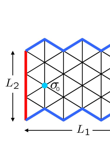
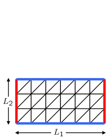
Refer to caption
Figure 10: A triangular lattice of size L1×L2subscript𝐿1subscript𝐿2L_{1}\times L_{2} with periodic boundary conditions; the red and the blue ends are identified, respectively. This lattice is symmetric w.r.t. each of vertical axes.
Refer to caption
Figure 11: A triangular lattice constructed from a square lattice by addition of diagonal edges. Its periodic structure is indicated by coloring as in fig.11.
Refer to caption
Figure 12: An illustration of the fact that those lattices given in figs.11 and 11 are equivalent iff L1subscript𝐿1L_{1} is a multiple of 2L22subscript𝐿22L_{2}. Here L1=6subscript𝐿16L_{1}=6 and L2=3subscript𝐿23L_{2}=3.
Refer to caption
Figure 13: A Z2subscript𝑍2Z_{2}-twist represented by a blue loop on the dual (hexagonal) lattice. On the original (triangular) lattice, it is represented by a stacked set of links (colored in red) with couplings of opposite sign.

Let us define a twist on a planar triangular lattice. A twist is a closed loop on the dual lattice, and the dual of a triangular lattice is a honeycomb (or hexagonal) lattice as shown in fig.13. Note that the blue line in fig.13 is a closed loop owing to the periodic structure of the lattice. It becomes, on the original lattice, a stacked set of links with a coupling constant of opposite sign, which is depicted as a set of red links in fig.13. Note that introducing a twist to a periodic lattice as in fig.13 is equivalent to imposing an anti-periodic boundary condition in the horizontal direction.

Let us remember that it is not the number of the walls but rather the number mod 2 of them that is physically relevant. This ‘Z2subscript𝑍2Z_{2} conservation’ of walls is a direct consequence of σ2=1superscript𝜎21\sigma^{2}=1 in the present model, and we can show it explicitly by a sequence of changes of variables σσ𝜎𝜎\sigma\to-\sigma. For instance, the partition function containing one wall and that containing three walls agree completely as illustrated in fig.14 in which red segments represent twisted links.
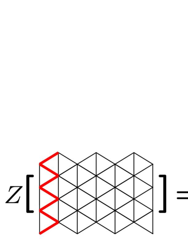
Refer to caption
Figure 14: The partition function does not differ for any odd number of twists, owing to the Z2subscript𝑍2Z_{2} conservation of the twist.

Exact expressions for partition functions of a planar triangular Ising model with various boundary conditions were derived by Wu and Hu via ‘Grassmann path integral method’ [39]. Let ZΛsubscript𝑍ΛZ_{\Lambda} (ZΛ()subscriptsuperscript𝑍ΛZ^{(-)}_{\Lambda}) denote the partition function with periodic boundary condition in both directions (with periodic in vertical and anti-periodic in horizontal direction), respectively. On a triangular lattice, three different couplings can be defined in each directions, so let us introduce J1subscript𝐽1J_{1} as the coupling constant on vertical bonds in figs.11,11 and J2,J3subscript𝐽2subscript𝐽3J_{2},J_{3} the other two. Reflection positivity however requires J2=J3(J)subscript𝐽2annotatedsubscript𝐽3absent𝐽J_{2}=J_{3}\,(\equiv J). Introduce

t1tanh(J1/kBT),ttanh(J/kBT).formulae-sequencesubscript𝑡1subscript𝐽1subscriptkB𝑇𝑡𝐽subscriptkB𝑇t_{1}\equiv\tanh(J_{1}/{\rm{k_{B}}}T),\ \ t\equiv\tanh(J/{\rm{k_{B}}}T). (170)

Our convention is such that t(1)>0subscript𝑡10t_{(1)}>0 corresponds to ferromagnetic coupling. On the (t,t1)𝑡subscript𝑡1(t,t_{1})-plane, there is a line which corresponds to T=Tc𝑇subscript𝑇𝑐T=T_{c} and we will call it the “critical line” in the following. Under the change of notation L1Nsubscript𝐿1𝑁L_{1}\to N and L2Msubscript𝐿2𝑀L_{2}\to M, the result due to Hu and Wu for this case reads

ZΛsubscript𝑍Λ\displaystyle Z_{\Lambda} = 1 2[2cosh3(βJ)]MN[Ω12,12+Ω12,0+Ω0,12sgn(TTc)Ω0,0],absentsuperscript1absentsubscript2absentsuperscriptdelimited-[]2superscript3𝛽𝐽𝑀𝑁delimited-[]subscriptΩ1212subscriptΩ120subscriptΩ012sgn𝑇subscript𝑇𝑐subscriptΩ00\displaystyle=\displaystyle\frac{\,1\,^{\mathstrut}}{\,2\,_{\mathstrut}}\left[2\cosh^{3}(\beta J)\right]^{MN}\Big{[}\Omega_{\frac{1}{2},\frac{1}{2}}+\Omega_{\frac{1}{2},0}+\Omega_{0,\frac{1}{2}}-\textrm{sgn}\,(T-T_{c})\Omega_{0,0}\Big{]}, (171)
ZΛ()superscriptsubscript𝑍Λ\displaystyle Z_{\Lambda}^{(-)} = 1 2[2cosh3(βJ)]MN[Ω12,12+Ω12,0Ω0,12+sgn(TTc)Ω0,0],absentsuperscript1absentsubscript2absentsuperscriptdelimited-[]2superscript3𝛽𝐽𝑀𝑁delimited-[]subscriptΩ1212subscriptΩ120subscriptΩ012sgn𝑇subscript𝑇𝑐subscriptΩ00\displaystyle=\displaystyle\frac{\,1\,^{\mathstrut}}{\,2\,_{\mathstrut}}\left[2\cosh^{3}(\beta J)\right]^{MN}\Big{[}\Omega_{\frac{1}{2},\frac{1}{2}}+\Omega_{\frac{1}{2},0}-\Omega_{0,\frac{1}{2}}+\textrm{sgn}\,(T-T_{c})\Omega_{0,0}\Big{]}, (172)

where

Ωμν=(A0)MN/2p=0M1q=0N1[1Bcos 2π(p+μ)MAcos 2π(q+ν)NAcos( 2π(p+μ)M 2π(q+ν)N)]1/2,subscriptΩ𝜇𝜈superscriptsubscript𝐴0𝑀𝑁2superscriptsubscriptproduct𝑝0𝑀1superscriptsubscriptproduct𝑞0𝑁1superscriptdelimited-[]1𝐵2𝜋superscript𝑝𝜇absentsubscript𝑀absent𝐴2𝜋superscript𝑞𝜈absentsubscript𝑁absent𝐴2𝜋superscript𝑝𝜇absentsubscript𝑀absent2𝜋superscript𝑞𝜈absentsubscript𝑁absent12\Omega_{\mu\nu}=(A_{0})^{MN/2}\prod_{p=0}^{M-1}\prod_{q=0}^{N-1}\Big{[}1-B\cos\displaystyle\frac{\,2\pi(p+\mu)\,^{\mathstrut}}{\,M\,_{\mathstrut}}-A\cos\displaystyle\frac{\,2\pi(q+\nu)\,^{\mathstrut}}{\,N\,_{\mathstrut}}-A\cos\Big{(}\displaystyle\frac{\,2\pi(p+\mu)\,^{\mathstrut}}{\,M\,_{\mathstrut}}-\displaystyle\frac{\,2\pi(q+\nu)\,^{\mathstrut}}{\,N\,_{\mathstrut}}\Big{)}\Big{]}^{1/2}, (173)
A0=(1+t2t1)2+(t1+t2)2+2t2(1+t1)2,A=2(1t12)(1t2)tA0,B=2t1(1t2)2A0formulae-sequencesubscript𝐴0superscript1superscript𝑡2subscript𝑡12superscriptsubscript𝑡1superscript𝑡222superscript𝑡2superscript1subscript𝑡12formulae-sequence𝐴21superscriptsubscript𝑡121superscript𝑡2𝑡subscript𝐴0𝐵2subscript𝑡1superscript1superscript𝑡22subscript𝐴0A_{0}=(1+t^{2}t_{1})^{2}+(t_{1}+t^{2})^{2}+2t^{2}(1+t_{1})^{2},\ \ \ A=\frac{2(1-t_{1}^{2})(1-t^{2})t}{A_{0}},\ \ \ B=\frac{2t_{1}(1-t^{2})^{2}}{A_{0}} (174)

with Tcsubscript𝑇𝑐T_{c} the phase-transition temperature. Using the formulae given above, we can show

Lemma 6.

In the disordered phase (T>Tc)(\ \Leftrightarrow T>T_{c}\ ) we have

limMlimN(1ZΛ()ZΛ)1/N=eρ,subscript𝑀subscript𝑁superscript1subscriptsuperscript𝑍Λsubscript𝑍Λ1𝑁superscripte𝜌\lim_{M\to\infty}\lim_{N\to\infty}\left(1-\frac{Z^{(-)}_{\Lambda}}{Z_{\Lambda}}\right)^{1/N}={\mathrm{e}}^{-\rho}, (175)

where

ρcosh1(g(B)|A|)>0,𝜌superscript1𝑔𝐵𝐴0\displaystyle\rho\equiv\cosh^{-1}\left(\frac{g(B)}{|A|}\right)>0, (176)
g(x){2x(1+x)(1<x<13)1x2(13x<1).\displaystyle g(x)\equiv\left\{\begin{matrix}\sqrt{-2x(1+x)}&\displaystyle\left(-1<x<-\frac{1}{3}\right)\\ \displaystyle\frac{1-x}{2}&\displaystyle\left(-\frac{1}{3}\leq x<1\right)\end{matrix}\right.. (177)

The order of two limits in (175) must not be changed.

In the above, g(B)|A|1𝑔𝐵𝐴1\displaystyle\frac{g(B)}{|A|}\geq 1 and |B|<1𝐵1|B|<1 are implicitly assumed; these can be shown for every (t,t1)(1,1)2𝑡subscript𝑡1superscript112(t,t_{1})\in(-1,1)^{2} by elementary methods. (Note that g(B)|A|=1𝑔𝐵𝐴1\displaystyle\frac{g(B)}{|A|}=1 defines the critical line.) The proof of theorem 6 is elementary but technically cumbersome, which we relegate to the appendix.

To gain an intuitive understanding of the above result, let us see fig.15, in which the projection of 1eρ1superscripte𝜌1-{\mathrm{e}}^{-\rho} onto the (t1,t)subscript𝑡1𝑡(t_{1},t)-plane is drawn. The black region corresponds to the (anti-)ferromagnetically ordered phase, while the colored region to the disordered phase. Brighter color represents larger ρ𝜌\rho, hence larger mass gap.

Refer to caption
Figure 15: The projection of 1eρ1superscripte𝜌1-{\mathrm{e}}^{-\rho} onto the (t1,t)subscript𝑡1𝑡(t_{1},t)-plane. The black region corresponds to the (anti-)ferromagnetically ordered phase and the colored region to the disordered phase. Brighter (darker) color represents larger (smaller) ρ𝜌\rho and especially ρ𝜌\rho diverges on the t=0𝑡0t=0 line. The boundary of the colored region signifies the critical line.

Fig.15 clearly shows a symmetry under tt𝑡𝑡t\leftrightarrow-t; this is a manifestation of the well-known fact that the triangular Ising model is invariant under simultaneous sign reversal of any two of J1,J2,J3subscript𝐽1subscript𝐽2subscript𝐽3J_{1},J_{2},J_{3}.

The inequality of our primary interest, namely (101) for the triangular Ising model, reads212121 Actually, we originally proved (101) on a square lattice, but the whole procedure of the proof goes over to the case of a triangular lattice almost unchanged.

σ0σnΛ2{ 1 2(1ZΛ()ZΛ)}n/N.\langle\sigma_{0}\sigma_{n}\rangle_{\Lambda}\leq 2\left\{\displaystyle\frac{\,1\,^{\mathstrut}}{\,2\,_{\mathstrut}}\left(1-\displaystyle\frac{\,Z_{\Lambda}^{(-)}\,{}^{\mathstrut}}{\,Z_{\Lambda}\,{}_{\mathstrut}}\right)\right\}^{n/N}. (178)

Letting M𝑀M\to\infty after N𝑁N\to\infty, we obtain

Theorem 6.
σ0σn2eρn.subscriptdelimited-⟨⟩subscript𝜎0subscript𝜎𝑛2superscripte𝜌𝑛\langle\sigma_{0}\sigma_{n}\rangle_{\infty}\leq 2{\mathrm{e}}^{-\rho n}. (179)

The above is the main result in this subsection; ρ𝜌\rho is a rigorous lower bound of the true mass gap. We should keep in mind that the l.h.s. of (178) is a pair correlation between two spins on the same horizontal level as depicted in fig.11; the two spins are not on the same lattice axis.

Since the exponential decay rates are equal for both sides of the inequality in the the square Ising model, it is natural to expect so in the triangular Ising model too. The asymptotic correlation between two spins on the same lattice axis in the triangular Ising model was derived by Stephenson for both ferromagnetic and antiferromagnetic couplings [40]. However, the asymptotic correlation between two spins off the axis is not found in the literature. We conjecture as follows:   Conjecture.
ρ𝜌\rho is equal to the true off-axis mass gap for every (t,t1)𝑡subscript𝑡1(t,t_{1}) in the disordered phase.   The most straightforward way to test the conjecture would be to measure the mass gap directly via Monte Carlo simulation. However, as already seen from (169) the exponential falloff generically receives power law corrections (the so-called ‘Ornstein-Zernike’ decay [41]) which makes a reliable fitting difficult. To evade this hamper would call for sophisticated methods such as the Monte Carlo Transfer Matrix Method [42]. A numerical check of the conjecture therefore seems to be a highly nontrivial task, and we defer it to future work.

In a special case, analytical test is possible: when t1=0subscript𝑡10t_{1}=0 the model reduces to the isotropic square Ising model and the off-axis correlation function reduces to the diagonal correlation function. From (176) it follows that

ρ|t1=0=cosh1(1+t2)24|t|(1t2)for|t|<tC=21,formulae-sequenceevaluated-at𝜌subscript𝑡10superscript1superscript1superscript𝑡224𝑡1superscript𝑡2for𝑡subscript𝑡𝐶21\rho\big{|}_{t_{1}=0}=\cosh^{-1}\frac{(1+t^{2})^{2}}{4|t|(1-t^{2})}\ \ \ \ \ \textrm{for}\ \ |t|<t_{C}=\sqrt{2\mathstrut}-1, (180)

which completely agrees with the exact diagonal mass gap obtained by Cheng and Wu in 1967 [36].

Further insight is gained by considering the isotropic case t=t1𝑡subscript𝑡1t=t_{1}. Since the two-point correlation function in this case is expected to be approximately isotropic (except for sign in antiferromagnetic case), it seems reasonable to compare eρsuperscripte𝜌{\mathrm{e}}^{-\rho} with e(3/2)msuperscripte32𝑚{\mathrm{e}}^{-(\sqrt{3}/2)m} where m𝑚m is the exact on-axis mass gap [40]. (3/232\sqrt{3\mathstrut}/2 is a geometric correction factor.)

Refer to caption
Figure 16: eρsuperscripte𝜌{\mathrm{e}}^{-\rho} and e(3/2)msuperscripte32𝑚{\mathrm{e}}^{-(\sqrt{3}/2)m} are plotted against t𝑡t in the case of isotropic case (t=t1𝑡subscript𝑡1t=t_{1}). Their agreement is remarkable especially at t𝑡t positive.

Fig.16 depicts the graphs of eρsuperscripte𝜌{\mathrm{e}}^{-\rho} and e(3/2)msuperscripte32𝑚{\mathrm{e}}^{-(\sqrt{3}/2)m} against t[1, 23]𝑡123t\in[-1,\,2-\sqrt{3\mathstrut}\,]. For t>0𝑡0t>0 they agree quite well; their nonzero difference is hardly discernible to the eye. For t<0𝑡0t<0 agreement is still not bad. To say the least, the comparison suggests that ρ𝜌\rho be fairly close to the true off-axis mass gap and supports, rather than defies, the conjecture.

It is readily seen from (177),(176) that eρsuperscripte𝜌{\mathrm{e}}^{-\rho} is a nonanalytic function in the region of negative t1subscript𝑡1t_{1}, which, assuming the validity of our conjecture, implies non-analyticity of the mass gap. Such an exotic possibility definitely deserves further study. Strictly speaking, however, there are different possibilities that cannot be denied here: for example it could be the case that ρ𝜌\rho equals the true mass gap only when t10subscript𝑡10t_{1}\geq 0. In the latter case, non-analyticity of ρ𝜌\rho does not signify that of the true mass gap.

Let us end this subsection by invoking the effectiveness of our approach. Although the circumstance concerning our conjecture is rather moot, it can be safely said that our result in this subsection is essentially new to the extent that it rigorously gives a lower bound for the still-unknown off-axis mass gap of the triangular (both ferromagnetic and antiferromagnetic, both isotropic and anisotropic) Ising model in the disordered phase.

3.6 Strong coupling analysis

In this section we show, using the convergent strong-coupling (taken as synonymous with high temperature) expansion, that both sides of the proved inequality (101) have an identical exponential decay rate at long distance as long as the on-axis correlation function is considered.222222 High-temperature behavior of correlation functions in Ising-like models have been studied by many authors in a variety of methods; see ref.[43], for example. It is worthwhile to note that a majority of existing studies deal with neither the off-axis correlation function nor the case of an antiferromagnetic coupling. Hopefully a partial understanding of this fact will be gained through the discusions in this subsection. The proof is valid in any dimension and makes no use of reflection positivity. Since the corresponding result in LGT has already been derived by Mu¨nsterM¨unster\rm{M\ddot{u}nster} [28] (as mentioned in section 2) and since no essential difficulty arises in extending his proof to the case of spin models, we shall be brief here and only try to sketch the main idea behind the approach. Implications of this result to our conjecture will be discussed later.

For simplicity of exposition let us consider the isotropic square Ising model and its on-axis correlation function (though our argument is readily extendable to more general models such as PCM). A precise statement of the claim goes follows: as long as the size of the lattice is larger enough than n𝑛n, the strong coupling expansion (SCE) of ρ𝜌\rho and m𝑚m are identical at least up to order n𝑛n. (Our notation is such that the definition of ρ𝜌\rho is in (175), m𝑚m is the mass gap, Z,Z(),L1,L2𝑍superscript𝑍subscript𝐿1subscript𝐿2Z,Z^{(-)},L_{1},L_{2} are the same as in section 165 and ttanh(J/kBT)𝑡𝐽subscriptkB𝑇t\equiv\tanh(J/{\rm{k_{B}}}T).)

Let us begin with the expression Z={σ}ij(1+tσiσj)𝑍subscript𝜎subscriptproduct𝑖𝑗1𝑡subscript𝜎𝑖subscript𝜎𝑗\displaystyle Z=\sum_{\{\sigma\}}\prod_{i\not=j}(1+t\sigma_{i}\sigma_{j}). Expanding Z𝑍Z into sums of disconnected loops and then taking the logarithm, we have logZ=γt|γ|𝑍subscript𝛾superscript𝑡𝛾\displaystyle\log Z=\sum_{\gamma}t^{|\gamma|} with γ𝛾\gamma any connected loop and |γ|𝛾|\gamma| the perimeter of γ𝛾\gamma. Using similar expression for Z()superscript𝑍Z^{(-)} we obtain logZ()Z=2γSt|γ|superscript𝑍𝑍2subscript𝛾𝑆superscript𝑡𝛾\displaystyle\log\frac{Z^{(-)}}{Z}=-2\sum_{\gamma\in S}t^{|\gamma|} where S𝑆S is the set of loops wrapping around the lattice in x1superscript𝑥1x^{1}-direction for odd number of times. Since we are interested in the limit |t|1much-less-than𝑡1|t|\ll 1, it is sufficient to consider only such loops that wind around the lattice in x1superscript𝑥1x^{1}-direction only once. Factorizing the degeneracy factor due to translational symmetry in x2superscript𝑥2x^{2}-direction, we have logZ()Z=2L2γSt|γ|superscript𝑍𝑍2subscript𝐿2subscript𝛾superscript𝑆superscript𝑡𝛾\displaystyle\log\frac{Z^{(-)}}{Z}=-2L_{2}\sum_{\gamma\in S^{\prime}}t^{|\gamma|}; the definition of Ssuperscript𝑆S^{\prime} should be obvious.

It is clear that the leading contribution, of order O(tL1)𝑂superscript𝑡subscript𝐿1O(t^{L_{1}}), comes from a straight line extending in x1superscript𝑥1x^{1}-direction while the subleading contributions come from loops which are formed via addition of some ‘decorations’ to the leading line. Dividing by the leading contribution and taking the logarithm will single out contributions of connected decorations, which is proportional to L1subscript𝐿1L_{1} owing to the translational invariance of the straight line. Thus we find exactly the behavior (148) in section 148:

log[(1L2logZ()Z)/tL1]L1.proportional-to1subscript𝐿2superscript𝑍𝑍superscript𝑡subscript𝐿1subscript𝐿1\log\Big{[}\left(\frac{1}{L_{2}}\log\frac{Z^{(-)}}{Z}\right)\Big{/}t^{L_{1}}\Big{]}\propto L_{1}. (181)

On the other hand, the on-axis two-point correlation function σxσx+rsubscriptdelimited-⟨⟩subscript𝜎𝑥subscript𝜎𝑥𝑟\langle\sigma_{x}\sigma_{x+r}\rangle_{\infty} can be written as a sum over contributions of lines connecting σ1subscript𝜎1\sigma_{1} to σ2subscript𝜎2\sigma_{2}, whose leading term comes from a straight line extending between σ1subscript𝜎1\sigma_{1} and σ2subscript𝜎2\sigma_{2} and subleading terms from zig-zag lines that descend from the leading one through addition of decorations. In this way we see that the SCE of

limL1,L2log[(1L2logZ()Z)/tL1]/L1(=ρlogt)annotatedsubscriptsubscript𝐿1subscript𝐿21subscript𝐿2superscript𝑍𝑍superscript𝑡subscript𝐿1subscript𝐿1absent𝜌𝑡\lim_{L_{1},L_{2}\to\infty}\log\Big{[}\left(\frac{1}{L_{2}}\log\frac{Z^{(-)}}{Z}\right)\Big{/}t^{L_{1}}\Big{]}\Big{/}L_{1}\ \ \ (=-\rho-\log t) (182)

is identical, term by term, to the SCE of limrlog[σxσx+r/tr]/r(=mlogt)annotatedsubscript𝑟subscriptdelimited-⟨⟩subscript𝜎𝑥subscript𝜎𝑥𝑟superscript𝑡𝑟𝑟absent𝑚𝑡\displaystyle\lim_{r\to\infty}\log\big{[}\langle\sigma_{x}\sigma_{x+r}\rangle_{\infty}/t^{r}\big{]}\big{/}r\ \ (=-m-\log t). Hence m=ρ𝑚𝜌m=\rho.

The argument above is valid for various other models as long as on-axis correlation functions are concerned. Then it is natural to ask about off-axis correlation functions. (This is the case relevant for the conjecture.) From fig.11 it is easily understood that the leading contribution to the SCE of 1L2logZ()Z1subscript𝐿2superscript𝑍𝑍\displaystyle\frac{1}{L_{2}}\log\frac{Z^{(-)}}{Z} does not come from a single straight line: instead it comes from (L1L1/2)matrixsubscript𝐿1subscript𝐿12\begin{pmatrix}L_{1}\\ L_{1}/2\end{pmatrix}different loops, all of the same length L1subscript𝐿1L_{1}. So we now have a number of different ways to see a given higher-order loop as a sum of any one of the leading-order loops and a decoration added to it! This implies that the counting of diagrams appearing in SCE of 1L2logZ()Z1subscript𝐿2superscript𝑍𝑍\displaystyle\frac{1}{L_{2}}\log\frac{Z^{(-)}}{Z} (and of off-axis correlation function, too) is immensely complicated. We even face another problem: since most of the leading-order loops have no translational symmetry, it becomes a nontrivial task to show (181). For these reasons we cannot give a mathematically rigorous proof of the conjecture even at sufficiently high temperature.

Some caveats are in order.

  • First, remember that we did confirm m=ρ𝑚𝜌m=\rho for the diagonal correlation function in the square Ising model ((180) and the accompanying discussion). This fact implies that our inability to prove (the very existence of m,ρ𝑚𝜌m,\ \rho and) the equality m=ρ𝑚𝜌m=\rho for off-axis correlation function in SCE approach does not itself constitute a disproof.

  • One may be tempted to argue that, since an exact one-to-one correspondence between the diagrams for SCE of σ1σ2subscriptdelimited-⟨⟩subscript𝜎1subscript𝜎2\langle\sigma_{1}\sigma_{2}\rangle_{\infty} and those for SCE of 1L2logZ()Z1subscript𝐿2superscript𝑍𝑍\displaystyle\frac{1}{L_{2}}\log\frac{Z^{(-)}}{Z} exists, m=ρ𝑚𝜌m=\rho would readily follow even in the off-axis case if we presume the existences of both m𝑚m and ρ𝜌\rho. This reasoning is however incorrect, because the exact correspondence is present only in the on-axis case. (This point is quite nontrivial.) An example of a loop that appears in SCE of 1L2logZ()Z1subscript𝐿2superscript𝑍𝑍\displaystyle\frac{1}{L_{2}}\log\frac{Z^{(-)}}{Z} as one of the leading contributions but has no counterpart among the diagrams in SCE of σ1σ2subscriptdelimited-⟨⟩subscript𝜎1subscript𝜎2\langle\sigma_{1}\sigma_{2}\rangle_{\infty} is shown in fig.17. (Although somewhat counterintuitive, this loop has a minimum perimeter to wind around the lattice in horizontal direction.)

    Since we have to send L1subscript𝐿1L_{1}\to\infty before L2subscript𝐿2L_{2}\to\infty in estimating ρ𝜌\rho, those loops can never be neglected. From this point of view, it is rather surprising that m=ρ𝑚𝜌m=\rho holds in the off-axis case of the square Ising model.

  • It seems worthwhile to note a qualitative difference between ferromagnetic and antiferromagnetic cases. The so-called random path representation σ1σ2=γt|γ|delimited-⟨⟩subscript𝜎1subscript𝜎2subscript𝛾superscript𝑡𝛾\displaystyle\langle\sigma_{1}\sigma_{2}\rangle=\sum_{\gamma}t^{|\gamma|}, where the sum runs over every path connecting σ1subscript𝜎1\sigma_{1} to σ2subscript𝜎2\sigma_{2}, loses its probabilistic interpretation when t|γ|<0superscript𝑡𝛾0t^{|\gamma|}<0. This actually happens in a triangular Ising model with antiferromagnetic couplings. In such a case it is impossible to apply fertile probability-theoretical methods, so that a particular difficulty is envisaged in settling the conjecture when the coupling is antiferromagnetic.

Summarizing above, we do not have a definitive answer as to the validity of the conjecture even at sufficiently high temperature, and further analysis on this topic will be hopefully reported elsewhere.
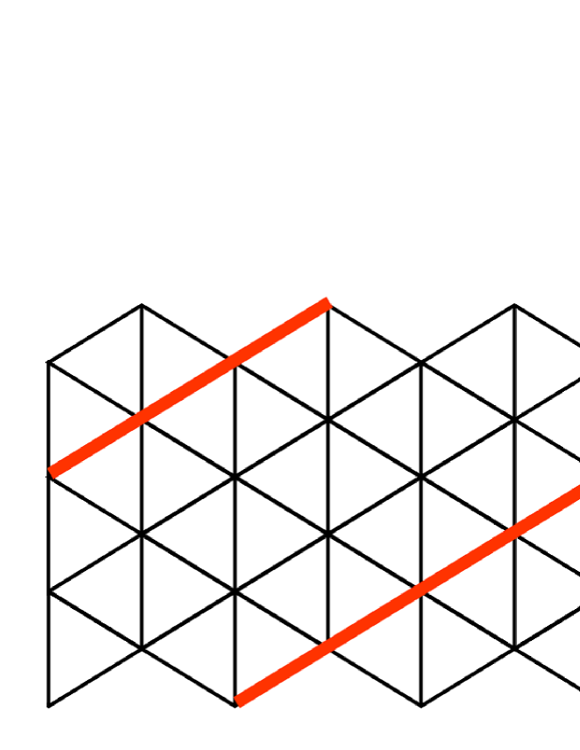
Refer to caption
Figure 17: Drawn in red is an example of a loop wrapped around the lattice in vertical as well as in horizontal direction. Such loops appear numerously if the horizontal size of the lattice is much larger than its vertical size.

4 Conclusion

In this paper we generalized the inequality of Tomboulis-Yaffe in SU(2)𝑆𝑈2SU(2) LGT to SU(N)𝑆𝑈𝑁SU(N) LGT and also to general classical spin systems, together with a detailed analysis of basic properties of non-Abelian twists. Our result is obtained essentially on a finite lattice and gives a rigorous upper bound of a Wilson loop and a two-point correlation function. An intriguing point is that the inequality obtained for spin models does not require the center of the symmetry group, so they can be applied e.g. to G×G𝐺𝐺G\times G PCM with centerless G𝐺G. This point seems to be a progress compared with preceding studies in which the center was perceived as special without physically convincing motivation232323Some arguments that allege the speciality of the center do exist in the literature, but they seem to be rather subtle, as discussed attentively in ref.[21]..

Furthermore we demonstrated our result explicitly in some solvable models and found in the square Ising model that the obtained lower bound of the mass gap is equal to the exact one. We also calculated the off-axis mass gap in the triangular Ising model for various couplings, but this time the exact mass gap is not known and direct comparison is impossible. We conjectured that the bound is indeed saturated and pointed out that the conjecture implies the non-analyticity of the mass gap. We have tested its validity in several ways, including strong coupling analysis, but a definitive conclusion is still lacking and is left for future work.

At present the mechanisms of the quark confinement in non-Abelian gauge theories and the mass gap generation in non-Abelian spin models still remain elusive, and we hope that our result will be useful for further clarification of the issue.

Note added

After this work was completed, we learned that C. Borgs and E. Seiler had already obtained a result very similar to theorem 2 of this paper; see Lemma II.8 and the accompanying discussion in ref.[44]242424 I thank E. Seiler for kindly pointing out this fact to me.. But since it links the Polyakov loop correlator and not the Wilson loop with the electric flux free energy, it is not quite the same as ours. It does, however, already imply the ’t Hooft’s string tension is less than or equal to Wilson’s (see (II.48) and (II. 50) of ref.[44]). Finally we note that their results hardly overlap with ours in section 3.

Acknowledgment

The author thanks Tetsuo Hatsuda, Yoshio Kikukawa, Seiji Miyashita, Masao Ogata, Shoichi Sasaki, Hiroshi Suzuki, Shun Uchino and Tamiaki Yoneya for enlightening discussions and Ming-Chya Wu for valuable correspondence concerning ref.[39]. Thanks also go to the anonymous referee for useful suggestions. This work was supported in part by Global COE Program “the Physical Sciences Frontier”, MEXT, Japan.

Appendix Appendix A Proof of Lemma 6

For T>Tc𝑇subscript𝑇𝑐T>T_{c}, (171) and (172) yield

ZΛZΛ()ZΛ+ZΛ()=Ω0,12Ω0,0Ω12,12+Ω12,0.\displaystyle\frac{\,Z_{\Lambda}-Z_{\Lambda}^{(-)}\,{}^{\mathstrut}}{\,Z_{\Lambda}+Z_{\Lambda}^{(-)}\,{}_{\mathstrut}}=\displaystyle\frac{\,\Omega_{0,\frac{1}{2}}-\Omega_{0,0}\,^{\mathstrut}}{\,\Omega_{\frac{1}{2},\frac{1}{2}}+\Omega_{\frac{1}{2},0}\,{}_{\mathstrut}}. (183)

Let us define θAB(μ,p,M)0superscriptsubscript𝜃𝐴𝐵𝜇𝑝𝑀0\theta_{A}^{B}(\mu,p,M)\geq 0 by

coshθAB(μ,p,M)|1Bcos 2π(p+μ)M|/|2Acosπ(p+μ)M|.superscriptsubscript𝜃𝐴𝐵𝜇𝑝𝑀1𝐵2𝜋superscript𝑝𝜇absentsubscript𝑀absent2𝐴𝜋superscript𝑝𝜇absentsubscript𝑀absent\cosh\theta_{A}^{B}(\mu,p,M)\equiv\Big{|}1-B\cos\displaystyle\frac{\,2\pi(p+\mu)\,^{\mathstrut}}{\,M\,_{\mathstrut}}\Big{|}\Big{/}\Big{|}2A\cos\displaystyle\frac{\,\pi(p+\mu)\,^{\mathstrut}}{\,M\,_{\mathstrut}}\Big{|}. (184)

It is tedious but straightforward to show that the minimum of coshθABsuperscriptsubscript𝜃𝐴𝐵\cosh\theta_{A}^{B} as a function of 1cosπ(p+μ)M11𝜋superscript𝑝𝜇absentsubscript𝑀absent1-1\leq\cos\displaystyle\frac{\,\pi(p+\mu)\,^{\mathstrut}}{\,M\,_{\mathstrut}}\leq 1 is given by g(B)|A|𝑔𝐵𝐴\displaystyle\frac{g(B)}{|A|} (see (177)), and that g(B)|A|1𝑔𝐵𝐴1\displaystyle\frac{g(B)}{|A|}\geq 1 for every (t,t1)(0,1)2𝑡subscript𝑡1superscript012(t,t_{1})\in(0,1)^{2}, with equality on the critical line. After elementary calculations, we find

(Ωμν)2(A0 2)MN{p=0M1|2Acosπ(p+μ)M|expθAB(μ,p,M)}Nsimilar-to-or-equalssuperscriptsubscriptΩ𝜇𝜈2superscriptsuperscriptsubscript𝐴0absentsubscript2absent𝑀𝑁superscriptconditional-setsuperscriptsubscriptproduct𝑝0𝑀1conditional2𝐴𝜋superscript𝑝𝜇absentsubscript𝑀absentsuperscriptsubscript𝜃𝐴𝐵𝜇𝑝𝑀𝑁(\Omega_{\mu\nu})^{2}\simeq\Big{(}\displaystyle\frac{\,A_{0}\,^{\mathstrut}}{\,2\,_{\mathstrut}}\Big{)}^{MN}\left\{\prod_{p=0}^{M-1}\Big{|}2A\cos\displaystyle\frac{\,\pi(p+\mu)\,^{\mathstrut}}{\,M\,_{\mathstrut}}\Big{|}\exp\theta_{A}^{B}(\mu,p,M)\right\}^{N} (185)

for N1much-greater-than𝑁1N\gg 1. Since (185) has no dependence on ν𝜈\nu,

limNΩ12,0Ω12,12=limNΩ0,0Ω0,12=1.\displaystyle\lim_{N\to\infty}\displaystyle\frac{\,\Omega_{\frac{1}{2},0}\,^{\mathstrut}}{\,\Omega_{\frac{1}{2},\frac{1}{2}}\,{}_{\mathstrut}}=\displaystyle\lim_{N\to\infty}\displaystyle\frac{\,\Omega_{0,0}\,^{\mathstrut}}{\,\Omega_{0,\frac{1}{2}}\,{}_{\mathstrut}}=1. (186)

Next, using (185) we get

Ω12,12Ω0,12exp{Nk=02M1(1)k+1fAB(k 2M)}for N1,\displaystyle\frac{\,\Omega_{\frac{1}{2},\frac{1}{2}}\,^{\mathstrut}}{\,\Omega_{0,\frac{1}{2}}\,{}_{\mathstrut}}\simeq\exp\Big{\{}N\displaystyle\sum_{k=0}^{2M-1}(-1)^{k+1}f_{A}^{B}\Big{(}\displaystyle\frac{\,k\,^{\mathstrut}}{\,2M\,_{\mathstrut}}\Big{)}\Big{\}}\hskip 30.0pt\textrm{for\ }N\gg 1, (187)

with

fAB(x) 1 2log{1Bcos(2πx)+(1Bcos(2πx))2(2Acos(πx))2}.superscriptsubscript𝑓𝐴𝐵𝑥superscript1absentsubscript2absent1𝐵2𝜋𝑥superscript1𝐵2𝜋𝑥2superscript2𝐴𝜋𝑥2f_{A}^{B}(x)\equiv\displaystyle\frac{\,1\,^{\mathstrut}}{\,2\,_{\mathstrut}}\log\Big{\{}1-B\cos(2\pi x)+\sqrt{\big{(}1-B\cos(2\pi x)\big{)}^{2}-\big{(}2A\cos(\pi x)\big{)}^{2}}\,\Big{\}}. (188)

Let us investigate how fast Ω0,0Ω0,12\displaystyle\frac{\,\Omega_{0,0}\,^{\mathstrut}}{\,\Omega_{0,\frac{1}{2}}\,{}_{\mathstrut}} converges to 1. Using (185) we can show

(Ω0,0Ω0,12)2p=0M1{14exp(NθAB)}for N1.\Big{(}\displaystyle\frac{\,\Omega_{0,0}\,^{\mathstrut}}{\,\Omega_{0,\frac{1}{2}}\,{}_{\mathstrut}}\Big{)}^{2}\simeq\sideset{}{}{\prod}_{p=0}^{M-1}\Big{\{}1-4\exp(-N\theta_{A}^{B})\Big{\}}\hskip 40.0pt\textrm{for\ \,}N\gg 1. (189)

Define θ¯¯𝜃\overline{\theta} as the smallest of {θAB(0,p,M)}psubscriptsuperscriptsubscript𝜃𝐴𝐵0𝑝𝑀𝑝\{\theta_{A}^{B}(0,p,M)\}_{p}. Then (189) simplifies to

(Ω0,0Ω0,12)21KeNθ¯for N1.\Big{(}\displaystyle\frac{\,\Omega_{0,0}\,^{\mathstrut}}{\,\Omega_{0,\frac{1}{2}}\,{}_{\mathstrut}}\Big{)}^{2}\simeq 1-K\,{\mathrm{e}}^{-N\overline{\theta}}\hskip 30.0pt\textrm{for\ \,}N\gg 1. (190)

K𝐾K is an integer {4,8,12,16}absent481216\in\{4,8,12,16\}, dependent on A,B𝐴𝐵A,\,B and M𝑀M. Substitution of (186), (187) and (190) into (183) yields

1ZΛ()ZΛ2exp{N[θ¯+k=02M1(1)k+1fAB(k 2M)]}for N1.1-\displaystyle\frac{\,Z_{\Lambda}^{(-)}\,{}^{\mathstrut}}{\,Z_{\Lambda}\,{}_{\mathstrut}}\simeq 2\exp\Big{\{}-N\Big{[}\overline{\theta}+\displaystyle\sum_{k=0}^{2M-1}(-1)^{k+1}f_{A}^{B}\Big{(}\displaystyle\frac{\,k\,^{\mathstrut}}{\,2M\,_{\mathstrut}}\Big{)}\Big{]}\Big{\}}\hskip 30.0pt\textrm{for\ \,}N\gg 1. (191)

Since θ¯=cosh1(g(B)|A|)+O( 1M)¯𝜃superscript1𝑔𝐵𝐴𝑂superscript1absentsubscript𝑀absent\displaystyle\overline{\theta}=\cosh^{-1}\left(\frac{g(B)}{|A|}\right)+O\Big{(}\displaystyle\frac{\,1\,^{\mathstrut}}{\,M\,_{\mathstrut}}\Big{)} and k=02M1(1)k+1fAB(k 2M)=O( 1M)superscriptsubscript𝑘02𝑀1superscript1𝑘1superscriptsubscript𝑓𝐴𝐵superscript𝑘absent2subscript𝑀absent𝑂superscript1absentsubscript𝑀absent\displaystyle\sum_{k=0}^{2M-1}(-1)^{k+1}f_{A}^{B}\Big{(}\displaystyle\frac{\,k\,^{\mathstrut}}{\,2M\,_{\mathstrut}}\Big{)}=O\Big{(}\displaystyle\frac{\,1\,^{\mathstrut}}{\,M\,_{\mathstrut}}\Big{)} for M1much-greater-than𝑀1M\gg 1, we find

limMlimN(1ZΛ()ZΛ)1/N=eρ,\displaystyle\lim_{M\to\infty}\lim_{N\to\infty}\left(1-\displaystyle\frac{\,Z_{\Lambda}^{(-)}\,{}^{\mathstrut}}{\,Z_{\Lambda}\,{}_{\mathstrut}}\right)^{1/N}={\mathrm{e}}^{-\rho}, (192)
ρcosh1(g(B)|A|),𝜌superscript1𝑔𝐵𝐴\displaystyle\rho\equiv\cosh^{-1}\left(\frac{g(B)}{|A|}\right), (193)

which is the desired result. \square

References

  • [1] E. T. Tomboulis, L. G. Yaffe, Commun. Math. Phys. 100 (1985) 313.
  • [2] R. Peierls, Proc. Cambridge Phil. Soc. 32 (1936) 477.
  • [3] L. Onsager, Phys. Rev. 65 (1944) 117; Nuovo Cimento (Suppl.) 6 (1949) 261.
  • [4] J. M. Kosterlitz, D. J. Thouless, J. Phys. C6 (1973) 1181; see also V. L. Berezinskii, Sov. Phys. JETP 34 (1972) 610.
  • [5] G. ’t Hooft, Nucl. Phys. B138 (1978) 1; ibid. B153 (1979) 141.
  • [6] G. Mack, V. B. Petkova, Annals Phys. 125 (1980) 117.
  • [7] T. Yoneya, Nucl. Phys. B144 (1978) 195; J. M. Cornwall, Nucl. Phys. B157 (1979) 392; H. B. Nielsen, P. Olesen, Nucl. Phys. B160 (1979) 380.
  • [8] B. Svetitsky, L. G. Yaffe, Nucl. Phys. B210[FS6] (1982) 423.
  • [9] F. Bursa, M. Teper, JHEP 08 (2005) 060 [arXiv:hep-lat/0505025]; Ph. de Forcrand, D. Noth, Phys. Rev. D72 (2005) 114501 [arXiv:hep-lat/0506005].
  • [10] R. L. Dobrushin, S. B. Shlosman, Commun. Math. Phys. 42 (1975) 31.
  • [11] L. G. Yaffe, Phys. Rev. D21 (1980) 1574.
  • [12] J. Groeneveld, J. Jurkiewicz, C. P. Korthals Altes, Phys. Scripta 23 (1981) 1022.
  • [13] P. A. Lee, T. V. Ramakrishnan, Rev. Mod. Phys. 57 (1985) 287 and references therein.
  • [14] H. Iida, T. Doi, N. Ishii, H. Suganuma, K. Tsumura, Phys. Rev. D74 (2006) 074502 [arXiv:hep-lat/0602008].
  • [15] F. Green, S. Samuel, Nucl. Phys. B190[FS3] (1981) 113.
  • [16] A. M. Polyakov, Gauge Fields and Strings, Harwood, 1987.
  • [17] P. Rossi, M. Campostrini, E. Vicari, Phys. Rept. 302 (1998) 143 [arXiv:hep-lat/9609003].
  • [18] L. Del Debbio, H. Panagopoulos, P. Rossi, E. Vicari, JHEP 01 (2002) 009 [arXiv:hep-th/0111090].
  • [19] T. Kova´csKov´acs\rm{Kov\acute{a}cs}, E. T. Tomboulis, Phys. Lett. B321 (1994) 75 [arXiv:hep-lat/9311005]; Phys. Lett. B367 (1996) 254 [arXiv:hep-lat/9508010]; Nucl. Phys. Proc. Suppl. 47 (1996) 290.
  • [20] T. Kova´csKov´acs\rm{Kov\acute{a}cs}, Nucl. Phys. B482 (1996) 613 [arXiv:hep-lat/9603022]; UCLA PhD Thesis (1996).
  • [21] O. A. Borisenko, P. Skala, Phys. Rev. D62 (2000) 014502.
  • [22] T. Kova´csKov´acs\rm{Kov\acute{a}cs}, E. T. Tomboulis, Phys. Rev. D65 (2002) 074501 [arXiv:hep-lat/0108017].
  • [23] I. Montvay, G. Mu¨nsterM¨unster\rm{M\ddot{u}nster}, Quantum fields on a lattice, Cambridge University Press, Cambridge, 1994.
  • [24] K. Osterwalder, E. Seiler, Ann. Phys. 110 (1978) 440.
  • [25] T. Kova´csKov´acs\rm{Kov\acute{a}cs}, E. T. Tomboulis, Phys. Rev. Lett. 85 (2000) 704 [arXiv:hep-lat/0002004].
  • [26] Ph. de Forcrand, M. D’Elia, M. Pepe, Phys. Rev. Lett. 86 (2001) 1438 [arXiv:hep-lat/0007034].
  • [27] Ph. de Forcrand, L. von Smekal, Phys. Rev. D66 (2002) 011504 [arXiv:hep-lat/0107018].
  • [28] G. Mu¨nsterM¨unster\rm{M\ddot{u}nster}, Nucl. Phys. B180[FS2] (1981) 23.
  • [29] E. T. Tomboulis, arXiv:0707.2179[hep-th].
  • [30] T. Kanazawa, Phys. Lett. B670 (2009) 421 [arXiv:0805.2742].
  • [31] K. R. Ito, E. Seiler, arXiv:0803.3019[hep-th].
  • [32] D. J. Gross, E. Witten, Phys. Rev. D21 (1980) 446.
  • [33] A. W. Knapp, Lie Groups Beyond an Introduction, 2nd ed., Birkha¨user,Birkh¨auser\rm{Birkh\ddot{a}user,} Boston, 2002.
  • [34] B. B. Beard, M. Pepe, S. Riederer, U.-J. Wiese, Comput. Phys. Commun. 175 (2006) 629 [arXiv:hep-lat/0602018].
  • [35] R. D. Pisarski, F. Wilczek, Phys. Rev. D29 (1984) 338.
  • [36] B. M. McCoy, T. T. Wu, The Two-Dimensional Ising Model, Harvard University Press, Cambridge, 1973; C. Itzykson, J.-M. Drouffe, Statistical field theory, Cambridge University Press, Cambridge, 1989; J. Palmer, Planar Ising Correlations, Progr. Math. Phys. 49, Birkha¨userBirkh¨auser{\rm{Birkh\ddot{a}user}}, Boston, 2007.
  • [37] B. Kastening, Phys. Rev. E66 (2002) 057103 [arXiv:cond-mat/0209544].
  • [38] R. M. F. Houtappel, Physica 16 (1950) 425.
  • [39] M.-C. Wu, C.-K. Hu, J. Phys. A35 (2002) 5189 [arXiv:cond-mat/0204217].
  • [40] J. Stephenson, J. Math. Phys. 11 (1970) 413; ibid. 420.
  • [41] M. Campanino, D. Ioffe, Y. Velenik, Probab. Theory Rel. Fields 125 (2003) no. 3, 305 [arXiv:math/0111274] and references therein.
  • [42] N. A. Alves, B. A. Berg, R. Villanova, Phys. Rev. B41 (1990) 383; N. A. Alves, B. A. Berg, R. Villanova, Phys. Rev. B43 (1991) 5846.
  • [43] P. J. Paes-Leme, Ann. Phys. 115 (1978) 367; R. Schor, Commun. Math. Phys. 59 (1978) 213; B. Simon, Commun. Math. Phys. 77 (1980) 111; M. O’Carroll, J. Stat. Phys. 34 (1984) 597; M. O’Carroll, Phys. Lett. B143 (1984) 188; J. Bricmont, J. Flo¨hlichFl¨ohlich\rm{Fl\ddot{o}hlich}, Nucl. Phys. B251[FS13] (1985) 517; J. Bricmont, J. Flo¨hlichFl¨ohlich\rm{Fl\ddot{o}hlich}, Commun. Math. Phys. 98 (1985) 553; J. Bricmont, J. Flo¨hlichFl¨ohlich\rm{Fl\ddot{o}hlich}, Nucl. Phys. B280[FS18] (1987) 385.
  • [44] C. Borgs, E. Seiler, Commun. Math. Phys. 91 (1983) 329.