Self-healing diffusion quantum Monte Carlo algorithms: methods for direct reduction of the fermion sign error in electronic structure calculations

Abstract

We develop a formalism and present an algorithm for optimization of the trial wave-function used in fixed-node diffusion quantum Monte Carlo (DMC) methods. The formalism is based on the DMC mixed estimator of the ground-state probability density. We take advantage of a basic property of the walker configuration distribution generated in a DMC calculation, to (i) project-out a multi-determinant expansion of the fixed-node ground-state wave function and (ii) to define a cost function that relates the fixed-node ground-state and the non-interacting trial wave functions. We show that (a) locally smoothing out the kink of the fixed-node ground-state wave-function at the node generates a new trial wave-function with better nodal structure and (b) we argue that the noise in the fixed-node wave-function resulting from finite sampling plays a beneficial role, allowing the nodes to adjust towards the ones of the exact many-body ground state in a simulated annealing-like process. Based on these principles, we propose a method to improve both single determinant and multi-determinant expansions of the trial wave-function. The method can be generalized to other wave-function forms such as pfaffians. We test the method in a model system where benchmark configuration interaction calculations can be performed and most components of the Hamiltonian are evaluated analytically. Comparing the DMC calculations with the exact solutions, we find that the trial wave-function is systematically improved. The overlap of the optimized trial wave function and the exact ground state converges to 100% even starting from wave-functions orthogonal to the exact ground state. Similarly, the DMC total energy and density converges to the exact solutions for the model. In the optimization process we find an optimal non-interacting nodal potential of density-functional-like form whose existence was predicted in a previous publication [Phys. Rev. B 77, 245110 (2008)]. Tests of the method are extended to a model system with a conventional Coulomb interaction where we show we can obtain the exact Kohn-Sham effective potential from the DMC data.

I Introduction

In diffusion quantum Monte Carlo (DMC) a trial wave-function is used to enforce both the antisymmetry of the electronic many-body wave-functionanderson79 ; ceperley80 ; reynolds82 and the nodal structure of the solution. In highly correlated materials, the accuracy of the trial wave-function becomes increasingly important and determines the success or failure of the method. Indeed, concerns about the fixed-node accuracy have tended to limit applications of DMC to pre-transition metal elements. The discovery and development of new methods to improve the trial wave-functions, ideally without great computational expense, is consequently highly desirable for almost all DMC calculations.

In DMC calculations the trial wave-function $\Psi_{T}({\bf R})$ is commonly a product of an antisymmetric function $\Phi_{T}({\bf R})$ and a Jastrow factor $e^{J({\bf R})}$. Usually $\Phi_{T}({\bf R})$ is a Slater determinant constructed with single particle Kohn-Sham orbitals from density functional theory (DFT) or from other mean field approaches such as Hartree-Fock. The Jastrow factor does not change the nodes, but accelerates convergence and improves the algorithm’s numerical stability. The Jastrow factor is optimized in a previous variational Monte Carlo (VMC) calculation. The DMC algorithm finds the lowest energy of the set of all wave-functions that share the nodes of $\Psi_{T}({\bf R})$. The exact ground-state energy will be obtained only if the exact nodes are provided. Since any change to an antisymmetric wave-function must result in a higher energy than the antisymmetric ground state, the energy obtained with arbitrary nodes is an upper bound to the exact ground-state energy.anderson79 ; reynolds82 Only in small systems is it currently possible to improve the nodes bajdich05 ; filippi00 ; umrigar07 ; rios06 ; luchow07 or even avoid the trial wave-function approach altogether.ceperley84 ; kalos00 ; zhang91 For small or weakly correlated systems, where other numerical approaches can compete, the utility of DMC as a method depends crucially on the accuracy of the trial wave-function. Multiple determinant, pfaffian,bajdich05 and back-flowrios06 wave-functions and geminal productsbeaudet are increasingly popular due to the improved accuracy.

To improve the DMC energy one must improve the nodal surface of the trial wave-function. However, to our knowledge, all algorithms for wave-function optimization are based on the VMC approach, with any improvement in the DMC energy occurring only as a side-effect. The use of VMC might be a limitation since VMC samples more frequently the regions of the wave-function that have larger probability density and are thus far from the nodes.luchow07 Accordingly, VMC based optimization methods improve first the wave-function at regions which are far from the nodes, while the nodes are only improved indirectly. It has been found, however, that VMC based optimization methods, in general, also improve the DMC energy.umrigar07 ; toulouse08 Nevertheless, a direct optimization of the DMC energy is desirable, and might have improved convergence properties compared to current indirect approaches.

While it has been shown by us and others that, within the single Slater determinant approach, the computational cost of an electronic update step in the DMC algorithm can have an almost linear scaling with the number of electrons,williamson ; reboredo05 ; alfe04 the use of these methods is limited if we do not find a better source of trial wave-functions than those obtained from mean-field approaches such as DFT. We recently showedrosetta that Kohn-Sham DFT wave-functions cannot be expected to yield good nodes in general. As correlations increase, Kohn-Sham DFT wave-functions can be bad sources of nodal surfaces.rosetta Indeed, we also found that as the size of the system increases, the nodal error of DFT wave-functions might be of the order of the triplet excitation energies, precluding the prediction of accurate optical propertiestiago08jpc even for simple carbon fullerenes. Accordingly, it is highly desirable to find a method to (i) obtain trial wave-functions with accurate nodal structures, (ii) retain the simplicity of a mean field approach, or (iii) use a minimum number of Slater determinants i.e., the wave-functions are compact and easily evaluated, (iv) directly optimize the nodes in DMC, and (v) improve the nodal structure systematically independently of the starting point. In this contribution we provide such a method.

In order to use DMC to find the best trial wave-function we overcome two major obstacles: (i) obtain a representation of the fixed-node ground-state DMC wave-function suitable for optimization of the nodes, and (ii) find a method to keep the trial wave-function compact in large systems by minimizing the number of determinants.

This work is the natural continuation of a recent article (Ref. rosetta, ) where we proved the existence of an optimal effective nodal potential for generating the orbitals in the determinants in the trial wave-function used in DMC. While some details are rederived here, we recommend reading Ref. rosetta, before this article. We previously provedrosetta that specific properties of the interacting ground state can be retained via minimization of cost functions in the set of pure-state non-interacting densities. Each cost function defines the gradient of an effective non-interacting potential which is optimized in a Newton-Raphson-like approach until the cost function reaches a minimum. In this paper we take the next step: we use known properties of the walker distribution function generated in a DMC run to define a cost function relating the non-interacting wave-functions with the fixed-node ground-state wave-function. This allows us to obtain, for example, the Kohn-Sham potential or an effective nodal potential from the DMC calculation. The method appears to be limited by the quality of the fit, the statistics that one can collect in DMC and the representability of the nodal surface, which becomes increasingly more demanding as the number of electrons in the system increases. Although this might limit the applicability of the method to systems with small electron counts, we note that DMC is readily parallelized with excellent scaling on modern computers. We also expect that improved sampling and optimization schemes can be constructed using the initial ideas and methods presented here and in Ref. rosetta, .

The remainder of this paper is organized as follows. In Section II we demonstrate that the nodes can be improved by locally removing the kinks in the fixed-node ground state. In Section III we derive a formalism and a method to obtain a multi-determinant expansion of the fixed-node ground-state wave-function directly from a DMC run. For many applications, this expansion may already be sufficient. In Section IV we present a cost function that allows the optimization of more compact trial wave-functions that match the fixed-node ground state. A formalism for wave-function optimization based on an effective DFT-like nodal potential is given. In Section V we apply and compare these methods to a model system that can be solved nearly analytically and demonstrate its convergence properties. In Section VI we propose a general algorithm based on the experience gathered solving the model. Finally in Section VII we summarize and discuss the prospects of this method for application in large systems.

II Systematic reduction of the nodal error within DMC

The importance sampling DMC algorithm, in the fixed-node approximation, finds the lowest energy fn:energy $E^{DMC}_{T}$ among the set of all wave-functions that share the nodal surface $S_{T}({\bf R})$ where the trial wave-function $\Psi_{T}({\bf R})=0$ and changes sign. The symbol ${\bf R}$ denotes a point in the many-body $3N$ dimensional space of electron coordinates. We denote this wave-function $\Psi_{FN}({\bf R})$ as the fixed-node ground state. It can be shown that $\Psi_{FN}({\bf R})$ corresponds to the ground state of the interacting Hamiltonian containing an additional infinite external potential located at the nodes of $\Psi_{T}({\bf R})$.

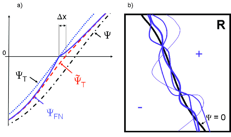
Figure 1: a) (Color online) Schematic representation of trial wave-function ($\Psi_{T}$, blue dots), fixed-node ground-state ($\Psi_{FN}$, purple continuous), ground-state ($\Psi$, black dash and dots), and new trial wave-function ($\tilde{\Psi}_{T}$, red dashed line) in the direction perpendicular to the nodal surface ($x$). We show that smoothing the kink in the fixed-node wave-function $\Psi_{FN}$ moves the nodes of $\tilde{\Psi}_{T}$ towards the nodes of the ground state $\Psi$ . b) Schematic representation of how the nodal surface evolves, shown with increasing purple line thickness, after each iteration in the algorithm. The noise introduced in the nodes by random fluctuations of the walkers is assumed to correct itself if the statistics is increased from one iteration to the next.

The gradient of the fixed-node ground-state wave-function $\Psi_{FN}({\bf R})$ can be discontinuous at the nodal surface $S_{T}({\bf R})$.reynolds82 Indeed, if the nodes of the trial wave-function do not correspond exactly to the nodes $S({\bf R})$ of an eigenstate of the Hamiltonian, the Laplacian of the fixed-node ground-state wave-function must have a $\delta({\bf R})$ contribution at least on part of $S_{T}({\bf R})$. Otherwise, since the time independent Schrödinger equation is satisfied elsewhere by $\Psi_{FN}({\bf R})$ with an energy $E^{DMC}_{T}$, without this delta in the Laplacian at the nodal surface, $\Psi_{FN}({\bf R})$ would be an eigenstate of the Hamiltonian. This implies that the gradient of $\Psi_{FN}({\bf R})$ must be discontinuous at least at one point of $S_{T}({\bf R})$ if the nodal surface $S_{T}({\bf R})\neq S({\bf R})$.

In Fig. 1a we show a schematic representation of the trial wave-function $\Psi_{T}({\bf R})$, the ground-state wave-function $\Psi({\bf R})$ and the fixed-node ground-state $\Psi_{FN}({\bf R})$. In this section we show that when this kink in $\Psi_{FN}({\bf R})$ is locally smoothed away as

$$\tilde{\Psi}_{T}({\bf R}) = \int{\bf dR^{\prime}}\Psi_{FN}({\bf R^{\prime}})\tilde{\delta}\left({\bf R^{\prime}-R}\right)$$

$$= \int{\bf dR^{\prime}}\Psi_{FN}({\bf R+R^{\prime}})\tilde{\delta}\left({\bf R^{\prime}}\right),\;$$

the nodes of the resulting functions improve for a broad class of $\tilde{\delta}\left({\bf R-R^{\prime}}\right)$.

Provided that $\Psi_{FN}$ is an antisymmetric function with finite projection on the ground state $\Psi_{0}$, it has been shownanderson79 ; HLRbook that $\Psi$, and its nodes converge to the exact ground state

$$\Psi=\lim_{t\rightarrow\infty}e^{-t(\hat{\mathcal{H}}-E_{T})}\Psi_{FN}$$ (2)

where $\hat{\mathcal{H}}$ is the Hamiltonian and $E_{T}$ is an estimate for the ground-state energy. Setting $t=M\tau$ in Eq. (2) yields the equivalent equation

$$\Psi=\lim_{M\rightarrow\infty}\left(e^{-\tau(\mathcal{H}-E_{T})}\right)^{M}\Psi_{FN}\;.$$ (3)

In the limit of small $\tau$ a real-space linear-order expansion of $e^{-\tau(\mathcal{H}-E_{T})}$ takes the form

$$\tilde{\delta}\left({\bf R^{\prime}-R}\right) = (2\pi\tau)^{\frac{-3N}{2}}e^{-\tau\left(V({\bf R})-E_{T}\right)}e^{\frac{-({\bf R-R^{\prime}})^{2}}{2\tau}}$$ (4)

$$\simeq \sum_{n}e^{-\tau(E_{n}-E_{T})}\left|\Psi_{n}\right>\left<\Psi_{n}\right|$$

where $V({\bf R})$ is the potential energy term (including interactions) in the Hamiltonian and the $E_{n}$ are eigenvalues of the eigenvectors $\Psi_{n}$. Replacing the first line in Eq. (4) in Eq. (II) we obtain a function $\tilde{\Psi}_{T}({\bf R})$ that has, by construction [see Eq. (4) second line], an energy less than or equal to the energy of $\Psi_{FN}({\bf R^{\prime}})$ (being equal for $S_{T}({\bf R})=S({\bf R})$). This form of trial wave-function is similar to a shadow wave-function.shadow ; fn:purediff If we could evaluate Eq. (II) analyticallyfn:bosons and use the result $\tilde{\Psi}_{T}({\bf R})$ in a new DMC run, we would obtain a new fixed-node ground-state wave-function with an even lower DMC energy. This implies that the nodes of $\tilde{\Psi}_{T}({\bf R})$ are better than the ones of $\Psi_{T}({\bf R})$.

Note that Eq. (4) tends to the Dirac $\delta$ function as $\delta({\bf R})=(2\pi\tau)^{-3N/2}e^{-({\bf R-R^{\prime}})^{2}/2\tau}$ for $\tau\rightarrow 0$. The factor $e^{-\tau\left(V({\bf R})-E_{T}\right)}$ in Eq. (4) does not alter the nodes: it is a positive scalar function (only acts as a branching term in a one time step simulation). Accordingly, to linear order in $\tau$, only the Gaussian is required to improve the nodes. In turn the Gaussian factor can be replaced by any other approximation of the $\delta$ function as long as it does the same to the nodes of $\Psi_{FN}({\bf R})$ as some Gaussian for small $\tau$.

In order to determine the class of smoothing functions that move the node in Eq. (II) as a Gaussian, we consider a patch $dS({\bf R})$ of the nodal surface $S_{T}({\bf R})$ centered at ${\bf R_{S}}$ with a diameter small enough (so that it can be considered a flat hyper-plane) but much larger than $\sqrt{\tau}$. The integration of the 3N dimensional Gaussian in the directions of the hyper-plane leads to a one dimensional Gaussian $G(x/\sqrt{\tau})=e^{-x^{2}/2\tau}/\sqrt{2\pi\tau}$. Any approximation of $\delta({\bf R})$ after integration in $3N-1$ coordinates should result in a function $d(x)$ that can be rescaled and translated to satisfy the following properties:

$$\int d(x)dx=1\;\;\int xd(x)dx=0\;\text{and}\;\int x^{2}d(x)dx=1\;.$$ (5)

In the immediate vicinity of ${\bf R_{S}}$, the function $\Psi_{FN}({\bf R})$ depends only on the coordinate in the direction normal to the surface ${\bf n_{S}}$ defined as $x={\bf(R-R_{S})\cdot n_{S}}={\bf\Delta R\cdot n_{S}}$. For $x\rightarrow 0$ we can approximate

$$\Psi_{FN}({\bf R_{S}+\Delta R})\simeq\Psi_{FN}({\bf R_{S}})+c_{1}x+k_{1}|x| +$$

$$+c_{2}x^{2}+k_{2}(x-|x|)^{2}+O(x^{3})$$ (6)

and

$$\frac{d}{dx}\Psi_{FN}({\bf R_{S}+\Delta R})\simeq c_{1}+k_{1}\mathrm{sign}(x)+$$ (7)

$$+2c_{2}x+4\;k_{2}(x-|x|)+O(x^{2}).$$

In Eq. (II) the wave-function is expanded as a combination of a smooth function (with coefficients $c_{1}$ and $c_{2}$) plus a kink ($k_{1}$ and $k_{2}$). Replacing Eq. (II) and Eq. (7) into Eq. (II) and replacing the Gaussian by a generic approximation of $\delta(x)=d(x/\sqrt{\tau})/\sqrt{\tau}$ we get:

$$\tilde{\Psi}_{T}({\bf R_{S}})=k_{1}A[d]\sqrt{\tau}+O(\tau)$$ (8)

and the first derivative

$$\frac{d}{dx}\tilde{\Psi}_{T}({\bf R_{S}})=c_{1}+k_{1}S[d]+4k_{2}A[d]\sqrt{\tau}+O(\tau)$$ (9)

where $A[d]=\int|x|d(x)dx$ and $S[d]=\int\mathrm{sign}(x)d(x)dx$. Note that if $d(x)$ has the Gaussian form $A[G]=\sqrt{2/\pi}>0$ and $S[G]=0$. Using Eqs. (8) and (9) we can estimate the displacement of the node to be

$$\Delta x\simeq-\frac{k_{1}A[d]}{c_{1}+k_{1}S[d]}\sqrt{\tau}+O(\tau).$$ (10)

Therefore, for any symmetric approximation of the $\delta$ function $S[d]=0$, provided that $A[d]>0$, one can obtain the same displacement in the node as a Gaussian with $\tau^{\prime}=\pi A[d]^{2}\tau/2$. For a non-symmetric $d(x)$, the node will move in the same direction as long as the sign in the denominator of Eq. (10) does not change. However, a uniform rescaling of $\tau$ to match the Gaussian form will no longer be possible. That means that the node will move faster towards the exact node in some regions of the surface than in others.

Thus, as long as the approximation of the delta used for smoothing is a function of the distance only, with $A[d]>0$, one can find some Gaussian that moves the node in the same way for every patch $dS({\bf R})$. This movement corresponds to a better node. The restrictions in $d(x)$ can be alleviated by using a repeated convolution. Using the central limit theorem it can be shown that a recursive convolution of any approximation of $d(x)$ tends to a Gaussian as long as the Taylor expansion of its Fourier transform exists. Thus if the shape of $d(x)$ is not known the method would be more stable if it is applied sequentially.

In section III we will use a smoothing function of the form

$$\tilde{\delta}\left({\bf R,R^{\prime}}\right)=\sum_{n}^{\sim}\Phi_{n}({\bf R})\Phi_{n}^{*}({\bf R^{\prime}}),$$ (11)

where the $\Phi_{n}({\bf R})$ are continuous functions without kinks forming a complete basis and the “$\sim$” in $\sum_{n}^{\sim}$ means that only some elements are included in the sum (with a criterion described below). If the $\Phi_{n}({\bf R})$ in Eq. (11) are obtained from a non-interacting problem and the criterion for truncation is an energy cutoff, it can be shown that the resulting function is only a function of the distance ${\bf(R-R^{\prime})}^{2}$. Since in that limit only plane waves of large energy are added to Eq. (11) and all the lower plane waves are included in the lower energy components, the basis can be transformed with a unitary transformation into a plane-wave basis with a spherical cutoff in reciprocal space. If there is the same number of plane waves in any direction the results of Eq. (11) only depend on the distance which implies that $S[d]=0$.

Since we restrict the sum in Eq. (11) to fermionic antisymmetric $\Phi_{n}({\bf R})$, Eq. (11) expands an antisymmetrized deltafn:bosons . This form projects out any non-fermionic component introduced in the wave-function along the DMC algorithm as in the A-function approach used by Bianchi and collaborators.bianchi93

In Section IV we propose a simple interpolation scheme to smooth the node where the expansion used in Eq. (11) is not taken to the high energy cutoff limit. The fact that these smoothing methods work in practice suggests that the conditions to improve the nodes are extended beyond the exact equivalence to a Gaussian form.

Note that a discontinuity of the gradient of the fixed-node wave-function $\Psi_{FN}({\bf R})$ at the node impliesfn:purediff that, if walkers are distributed according to $\Psi_{FN}({\bf R})$ with the sign (or phase) of $\Psi_{FN}({\bf R})$, there will be more walkers in the vicinity of one side of the nodal surface than on the other. Accordingly, if these walkers are released in a pure diffusion algorithm,HLRbook for $\tau\rightarrow 0$ they will cross, on average, more from one side of the nodal surface than from the other. The nodes defined by the population of these signed walkersHLRbook would move in the same direction that would result from smoothing the kink in $\Psi_{FN}({\bf R})$ provided the time step is short enough and kinetic energy term in the Green’s function [Eq. (4)] is dominant. Consequently, the nodes can be improved by moving them in the direction of least “walker pressure” within a pure diffusion approach.

Any method to obtain $\Psi_{FN}({\bf R})$ from the walker distribution in a DMC runbianchi96 will carry the error of statistical fluctuations from using a finite sample of walkers. Even if the $\Psi_{FN}({\bf R})$ is forced to remain antisymmetric,bianchi96 the nodes might move in the wrong direction because of these fluctuations. We assume the method is robust against these random fluctuations when applied recursively, and can form the basis of an optimization process to improve the trial wave-function. Note that if incorrect fluctuations increase the kink in $\Psi_{FN}({\bf R})$ at the node, the probability to sample the correct fixed-node wave-function will remain higher and also the probability to move the node in the correct direction in successive iterations. Conversely, fluctuations that correctly improve the nodes will be reinforcedfn:reinforced in successive iterations. Since these fluctuations are reduced when the statistical sampling is improved, the nodal surfaces will converge to the true nodes if the statistics is improved from one iteration to the next (Fig. 1b). Note that we do not claim that this process is necessarily the most efficient optimization approach: more sophisticated iterative methods and optimization algorithms are clearly possible.

Summarizing, we should be able to improve the nodes systematically provided we can obtain the anti-symmetric function $\Psi_{FN}({\bf R})$ from the walker configurations (probability distribution) of a DMC calculation after convolution with a smoothing function.fn:relnode

III Determination of the fixed-node ground-state wave-function from the DMC probability distribution

III.1 Sampling the fixed-node ground-state wave-function

The distribution function of the walkers in an importance sampling DMC algorithm is given by:ceperley80

$$f({\bf R}) = \Psi_{T}^{*}({\bf R})\Psi_{FN}({\bf R})$$

$$= \lim_{N_{c}\rightarrow\infty}\frac{1}{N_{c}}\sum_{i}^{N_{c}}\delta\left({\bf R-R}_{i}\right)$$

where $\Psi_{T}({\bf R})$ typically has the Slater-Jastrow form

$$\Psi_{T}({\bf R})=e^{J({\bf R})}\Phi_{T}({\bf R});$$ (13)

in which $\Phi_{T}({\bf R})$ consists of a single determinant for each electronic spin component composed of single-particle orbitals. The results of this paper are also valid if $\Phi_{T}({\bf R})$ has a more general form such as consisting of multi-determinant expansions for each spin component and/or containing back-flow or two-particle pfaffians. The ${\bf R}_{i}$ in Eq. (III.1) correspond to the positions of an equilibrated ensemble of $N_{c}$ configurations in a DMC algorithm (we have set the weights equal to one for simplicity).

We note that $\Psi_{FN}({\bf R})$ in Eq. (III.1) can be rewritten as an antisymmetric function times the Jastrow factor $e^{J({\bf R})}$ as

$$\Psi_{FN}({\bf R}) = e^{J({\bf R})}e^{-J({\bf R})}\Psi_{FN}({\bf R})$$ (14)

$$= e^{J({\bf R})}\sum_{n}\lambda_{n}\langle{\bf R}|(\prod c^{{\dagger}}\prod c)|\Phi_{T}\rangle$$

$$= e^{J({\bf R})}\sum_{n}\lambda_{n}\Phi_{n}({\bf R})$$

where $\sum\lambda_{n}(\prod c^{{\dagger}}\prod c)|\Phi_{T}\rangle$ is a complete configuration interaction (CI) expansion in the basis of electron-hole pairs . Accordingly, in Eq. (14) the $\Phi_{n}({\bf R})$ are Slater determinants or pfaffiansbajdich05 obtained from replacing in $\Phi_{T}({\bf R})$ some of the occupied $\phi_{\nu}$ single particle functions by unoccupied $\phi_{n}$ functions, accordingly $\int{\bf dR}\Phi_{n}^{*}({\bf R})\Phi_{m}({\bf R})=\delta_{n,m}$.

In practice, the CI expansion can be truncated retaining, for example, only the $\Phi_{m}({\bf R})$ with a non-interacting energy below a given energy cutoff. The CI expansion in principle consists of all single, double, triple, quadruple and higher-order excitations. By analogy with conventional CI calculations, the higher-order excitations are expected to contribute less to the wave-function than low-order excitations. As the kinetic energy of higher-order excitations increases as compared with the interaction, their contribution to the ground-state wave-function decreases.

While a Jastrow factor $e^{J({\bf R})}$ is not formally required in a complete expansion of the wave-function in Eq. (14), it is believed that the introduction of a Jastrow factor limits the number of coefficients required in the multi-determinant expansion, due in part to the more efficient description of the electron-electron cusp. For some applications it may be desirable to not employ a Jastrow factor, since the extracted wave-function may be more easily used in later analysis.

Replacing Eq. (14) and Eq. (13) in Eq. (III.1) we obtain

$$f({\bf R})=e^{2J({\bf R})}\Phi_{T}^{*}({\bf R})\sum_{n}\lambda_{n}\Phi_{n}({\bf R}).$$ (15)

Borrowing a method from Optimized Effective Potentials (OEP) we define the following projectors:us ; note

$$\xi_{n}({\bf R})=e^{-2J({\bf R})}\frac{\Phi_{n}({\bf R})}{\Phi_{T}({\bf R})}.$$ (16)

Note that the projectors $\xi_{n}({\bf R})$ are symmetric (bosonic) functions.fn:bosons Replacing $f({\bf R})$ by Eq. (15), using the definition of $\xi_{n}({\bf R})$ [Eq. (16)] and the orthogonality condition it can be demonstrated that

$$\int{\bf dR}f({\bf R})\xi_{n}^{*}({\bf R})=\lambda_{n}\;.$$ (17)

Thus, the coefficients of the multi-determinant expansion Eq. (14) of the fixed-node DMC ground-state wave-function can be estimated directly as a sum over the total number of walkers $N_{c}$ along the DMC random walk, using the second line of Eq. (III.1), as

$$\langle\lambda_{n}\rangle=\frac{1}{N_{c}}\sum_{i=1}^{N_{c}}\xi_{n}^{*}({\bf R}_{i})\;\gamma({\bf R}_{i})$$ (18)

where

$$\gamma({\bf R}_{i})=\frac{-1+\sqrt{1+2|{\bf v}|^{2}\tau}}{|{\bf v}|^{2}\tau}\text{ with }{\bf v}=\frac{\nabla\Psi_{T}({\bf R}_{i})}{\Psi_{T}({\bf R}_{i})}.$$ (19)

For convenience we divided by the number of walkers $N_{c}$ in Eqs. (III.1) and (18) since the normalization constant of $\Psi_{FN}({\bf R})$ and the corresponding coefficients $\lambda_{n}$ is arbitrary. The factor $\gamma({\bf R}_{i})$ in Eq. (18) is a time step, $\tau$, correction derived following Ref. umrigar93, that corrects the divergences of the projectors $\xi_{n}({\bf R}_{i})$ at the nodes. This correction is not always applied to estimators (e.g. the local energy) but we find that it reduces the error of the wave-function coefficients. For an uncorrelated sample of walker configurations the error bar of the multi-determinant expansion can be determined from

$$\langle\lambda_{n}^{2}\rangle = \frac{1}{N_{c}}\sum_{i=1}^{N_{c}}|\xi_{n}({\bf R}_{i})|^{2}\gamma({\bf R}_{i})^{2}$$ (20)

$$\langle{\sigma_{n}}\rangle = \sqrt{\frac{\langle\lambda_{n}\rangle^{2}-\langle\lambda_{n}^{2}\rangle}{N_{c}}}$$

$$\lambda_{n} \simeq \langle\lambda_{n}\rangle\pm\frac{\langle{\sigma_{n}}\rangle}{\sqrt{N_{c}-1}}.$$

As $N_{c}\rightarrow\infty$ in Eq. (20) the error bar in the multi-determinant coefficients $\lambda_{n}$ goes to zero. As usual, the error bars can be used to monitor convergence of the calculation. While the eventual goal is to obtain small error bars, we found in practice it is better to start with $N_{c}$ small and then to slowly increase it with each iteration as the trial wave-function improves (see below).

By substituting Eqs. (III.1), (13), and (16) into Eq. (17) and defining the fixed-node function $\Phi_{FN}$ in terms of the trial function Jastrow and the fixed-node wave-function $\Psi_{FN}$

$$\Psi_{FN}({\bf R})=e^{J({\bf R})}\Phi_{FN}({\bf R})$$ (21)

one can obtain this expression

$$\lambda_{n}=\int{\bf dR}\Phi_{n}^{*}({\bf R})\Phi_{FN}({\bf R})$$ (22)

for $\lambda_{n}$. We define $\tilde{\Psi}_{T}({\bf R})$ to be the truncated expansion (denoted using $\sim$) of Eq. (14)

$$\tilde{\Psi}_{T}({\bf R})=e^{J({\bf R})}\sum_{n}^{\sim}\lambda_{n}\Phi_{n}({\bf R})\;.$$ (23)

Substituting Eq. (22) into Eq. (23) yields the equation

$$\tilde{\Psi}_{T}({\bf R})=e^{J({\bf R})}\int{\bf dR^{\prime}}\left[\sum_{n}^{\sim}\Phi_{n}({\bf R})\Phi_{n}^{*}({\bf R}^{\prime})\right]\Phi_{FN}({\bf R}^{\prime})\;.$$ (24)

In Section II we showed that the appearance of a smoothing function of the form of Eq. (11) as in the term in brackets in Eq. (24) will smooth the nodes of $\Phi_{FN}({\bf R}^{\prime})$ yielding better nodes for $\tilde{\Psi}_{T}({\bf R})$. Since the $\Phi_{n}({\bf R})$ are selected to be eigenvectors of a non-interacting problem, highly localized features of $\Phi_{FN}({\bf R})$ would require components with high eigenvalues. At the same time, resolving those details would require a large number of configurations to improve the statistics. Accordingly, we truncate the expansion in Eq. (23) to the coefficients with relative errors smaller than 25%. Note that as the statistics is improved, the error bars diminishes, the number of functions retained in Eq. (11) increases and so does the localization of $\tilde{\delta}\left({\bf R,R^{\prime}}\right)$. Thus the conditions to improve the nodes systematically as described in Section II are reached as the statistics improves.

III.2 Sampling the Jastrow factor

Instead of expressing $\Psi_{FN}({\bf R})$ as a product of the same Jastrow factor used in $\Psi_{T}({\bf R})$ times a different multi-determinant expansion, one can choose to optimize the Jastrow factor while using the same antisymmetric function $\Phi_{T}({\bf R})$. It is easy to show that there is a symmetric bosonic factor that turns $\Phi_{T}({\bf R})$ into $\Psi_{FN}({\bf R})$ which is formally given by

$$e^{\tilde{J}({\bf R})}=\frac{\Psi_{FN}({\bf R})}{\Phi_{T}({\bf R})}\;.$$ (25)

Replacing Eq. (14) in Eq. (25) we find

$$e^{\tilde{J}({\bf R})} = e^{J({\bf R})}\sum_{n}\lambda_{n}\frac{\Phi_{n}({\bf R})}{\Phi_{T}({\bf R})}$$ (26)

$$= e^{3J({\bf R})}\sum_{n}\lambda_{n}\xi_{n}({\bf R})\;.$$

Note that the product $e^{\tilde{J}({\bf R})}\Phi_{T}({\bf R})$ yields Eq. (14). While this shows that the projectors $\xi_{n}({\bf R})$ could be used to improve the Jastrow factor, since they diverge for $\Phi_{T}({\bf R})\rightarrow 0$, it is necessary to fit instead a continuous functional form using values away from the nodes where truncation and sampling errors play a dominant role (see Section IV).

Updating the multi-determinant expansion of the antisymmetric part of the new trial wave-function, see Eq. (23), alters the nodes because (i) the expansion is truncated and (ii) the coefficients of the multi-determinant expansion have a random error due to finite sampling in Eq. (18). On the other hand, updating the Jastrow factor, see Eq. (26), keeps the nodes fixed but reduces the number of determinants required and the overall computational cost. There is a compromise between accuracy and speed.reynolds82 A very good wave-function might have a very small variance in the local energy, but if it is expensive to evaluate one might obtain the same statistical error in less wall-clock time with a faster lower quality wave-function. In an ideal case, if the nodes are $v$-representable (see below and Ref. rosetta, ) only a single determinant is required to describe the fixed-node ground-state wave-function to sufficient accuracy. In practice, the form of the Jastrow factor $e^{\tilde{J}({\bf R})}$ is unknown, while an infinite multi-determinant expansion is infeasible. This implies that both the factors in Eq. (14) are required in general; an efficient scheme will optimize both the Jastrow factor and determinantal part of the wave-function. Particularly for the case of a metallic system, the cost of a multi-determinant expansion might be prohibitive due to the large number of low-energy excitations. In this case it might be preferable to concentrate on an optimized Jastrow factor.wood06

III.3 A simple self-healing DMC algorithm

We have formulated, for small systems, a working iterative algorithm based on a multi-determinant or multi-pfaffian expansion of the fixed-node ground-state wave-function. In this algorithm the calculated coefficients Eq. (18) of the expansion are used to form a new trial wave-function defined by Eq. (23). Initially the statistical errors present in $\lambda_{n}$ due to finite sampling appear to have a beneficial role, particularly when the initial trial wave-function has poor nodes. Note that in the limit of an infinite number of determinants in Eq. (23) with no statistical sampling errors in $\lambda_{n}$ the trial wave-function would exactly reproduce the fixed-node wave-function, and an iterative improvement of the nodes would not be possible. Statistical fluctuations in the coefficients $\lambda_{n}$ allow the nodes to move. In the next iteration regions near beneficial fluctuations are revisited by walkers while bad statistically insignificant fluctuations tend not to propagate or grow. This stability against random noise appears to be valid in practice. Thus, the statistical error in the coefficients plays the role of a random thermal fluctuation in a simulated annealing algorithm.correa05 It is ironic and remarkable that random errors can be used to eliminate systematic errors.

While it is relatively economical to calculate a large number of multi-determinants every autocorrelation length, as more determinants are included in the trial wave-function each time step of the DMC calculation becomes more demanding. Accordingly, for large or continuum systems a method to minimize the number of determinants used to represent a given nodal surface is required. This is described in the next section.

IV Derivation of the best nodal-effective potential from DMC

While a working multi-determinant algorithm can be constructed on the basis of the multi-determinant expansion of the previous section, a significant step forward can be taken using the theory developed in Ref. rosetta, and taking advantage of Eq. (III.1) to construct a new trial wave-function that can be evaluated more efficiently than the multi-determinant expansion Eq. (23). This method will be most effective when the initial single particle orbitals involved in $\Phi_{T}({\bf R})$ are poor, e.g. if the system is strongly correlated.

IV.1 A cost function for the DMC algorithm

Given a probability density $p({\bf R})$ and a binned statistical sample of $N_{c}$ configurations of the random variable ${\bf R}$, we can define a new random variable

$$\chi^{2}=\sum_{i}^{M}\frac{\left[n_{i}-N_{c}\Omega_{i}\bar{p}({\bf R}_{i})\right]^{2}}{N_{c}\Omega_{i}\bar{p}({\bf R}_{i})}$$ (27)

which is distributed by the Chi-squared distribution function.HLRbook In Eq. (27) $\Omega_{i}$ is the volume of the bin $i$, with $n_{i}$ configuration counts, $\bar{p}({\bf R}_{i})$ is the average of $p({\bf R})$ in $\Omega_{i}$ and $M$ is the number of bins.

Each term in Eq. (27) is the square deviation of $n_{i}$ divided by the expectation value of the mean. In the limit of large counts the square of the mean is expected to be equal to the square deviation for the Poisson distribution of counts in a bin. Accordingly, in $\chi^{2}$ relative deviations from the mean have the same impact independently of the absolute value of the probability density. We will take advantage of this property to replace a wave-function difficult to evaluate Eq. (III.1) by a simpler approximate one that retains key properties. Setting $n_{i}=N_{c}\Omega_{i}\bar{q}({\bf R}_{i})$ in Eq. (27), dividing by $N_{c}$ taking the limit $M\rightarrow\infty$, and using the mean value theorem, we find a cost function to compare two continuous distribution functions:

$$K_{pq}=\int{\bf dR}\frac{\left[q({\bf R})-p({\bf R})\right]^{2}}{p({\bf R})}\;.$$ (28)

We showed in Ref. rosetta, that if we wish to preserve properties, other than the density, cost functions can be defined relating the many-body ground-state $\Psi({\bf R})$ with a non-interacting wave-function $\Phi_{T}({\bf R})$. The walker distribution functionceperley80 given by Eq. (III.1) allows us to construct several cost functions relating the wave-function to optimize with the exact fixed-node ground-state $\Psi_{FN}({\bf R})$. Using Eq. (28) as a guide, we propose the following expression:

$$K_{DMC} = \int{\bf dR}\frac{\left|\mu\;\Psi_{T}({\bf R})\tilde{\Psi}_{T}({\bf R})-f({\bf R})\right|^{2}}{\left|\mu\;\Psi_{T}({\bf R})\tilde{\Psi}_{T}({\bf R})\right|}\times$$ (29)

$$\theta\left(f({\bf R})-\eta\right),$$

where $\tilde{\Psi}_{T}({\bf R})$ is a trial wave-function to be optimized, $\mu=\left[\int\Psi_{T}({\bf R})\tilde{\Psi}_{T}({\bf R}){\bf dR}\right]^{-1}$, $f({\bf R})$ is given by Eq. (15) with coefficients obtained from a previous DMC run using Eq. (18), $\theta(x)$ is the Heaviside function, and $\eta$ is a small positive n umber. Note in Eq. (29) that the first factor vanishes when $\tilde{\Psi}_{T}({\bf R})\rightarrow\Psi_{FN}({\bf R})$. Indeed, if $\tilde{\Psi}_{T}({\bf R})$ is constrained to have the nodal surface $S_{T}({\bf R})$ and the sign (or phase) of $\Psi_{T}({\bf R})$, the integral of the first factor in Eq. (29) measures the probability that the distribution of a given ensemble of walkers $f({\bf R})$ corresponds to the distributionHLRbook

$$\alpha({\bf R})=\mu\tilde{\Psi}_{T}({\bf R})\Psi_{T}({\bf R})\;.$$ (30)

In Eq. (29), we add an absolute value function in the denominator of the first factor and a Heaviside function in order to extend the set of $\tilde{\Psi}_{T}({\bf R})$ where the cost function can be evaluated beyond the fixed-node space. Note that, since $f({\bf R})>0$, while negative values for $\alpha({\bf R})$ are allowed, they are penalized in the numerator more than positive values. In Eq.  (29), we add $\mu$ to enforce $\int\alpha({\bf R}){\bf dR}=\int f({\bf R}){\bf dR}$ for any $\tilde{\Psi}_{T}({\bf R})$. In Eq. (29) the nodes of $\tilde{\Psi}_{T}({\bf R})$ can move within a distance [which depends on $\eta$ and $f({\bf R}$)] around $S_{T}({\bf R})$. Otherwise, if the zeros of the numerator and denominator of Eq. (29) do not match, the value of the cost function would rise to infinity. An additional effect of $\theta$ is that any kink of $\Psi_{FN}({\bf R})$ at the node is not enforced by the cost function in $\tilde{\Psi}_{T}({\bf R})$. Since $\tilde{\Psi}_{T}({\bf R})$ will be obtained from the minimum energy solution of a non-interacting problemrosetta and departures at the node are not penalized, it will interpolate smoothly avoiding a kink. Note that we can choose alternative cost function forms. For example, we can replace the denominator in Eq. (29) by $f({\bf R}$). This choice would simplify the derivatives of the cost function but it has a couple of disadvantages: First $f({\bf R})$ is expected to be a very noisy function when its magnitude is small, while the product of non-interacting $v$-representable wave-functions $\alpha({\bf R})=\mu\;\tilde{\Psi}_{T}({\bf R})\Psi_{T}({\bf R})$ is expected to be smooth (see IV.2) . We choose not to amplify the noise of $f({\bf R})$ in the denominator. Second, in Eq. (29) a small number for $\alpha({\bf R})$ outside the window defined by the Heaviside function is highly penalized which confines the node of $\tilde{\Psi}_{T}({\bf R})$ to remain inside the window where the Heaviside function is zero.

IV.2 Representability of the nodal surface

Given an interaction in a many-body system, the Hohenberg-Kohn theoremhohenberg establishes a functional correspondence between electronic densities $\rho({\bf r})$, external potentials $V({\bf r})$, and ground-state wave-functions $\Psi({\bf R})$. The subset of densities $\rho({\bf r})$ corresponding to a ground state of an interacting system under an external potential $V({\bf r})$ are denoted as pure state $v$-representable.parr A non-interacting pure state $v$-representable density is given instead by $\bar{\rho}({\bf r})=\sum_{\nu}|\phi_{\nu}\left({\bf r}\right)|^{2}$ where $\phi_{\nu}\left({\bf r}\right)$ are Kohn-Sham-likekohn single particle orbitals, or eigenvectors, of the single-particle Hamiltonian:

$$\left[-\frac{1}{2}{\bf\nabla}^{2}+\bar{V}\left({\bf r}\right)\right]\phi_{\nu}\left({\bf r}\right)=\varepsilon_{\nu}\phi_{\nu}\left({\bf r}\right),$$ (31)

where $\bar{V}\left({\bf r}\right)$ is an effective single particle potential. The lowest energy Slater determinant constructed with the solution of Eq. (31) is a many-body non-interacting ground state. For simplicity we denote those quantities that are simultaneously interacting and non-interacting $v$-representable as simply $v$-representable. In addition, certain quantities can be multi-determinant $v$-representable, meaning that they can be represented by a finite multi-determinant expansion constructed with the solutions of Eq. (31). Since, the ground-state density $\rho({\bf r})$ determines the ground-state wave-function $\Psi({\bf R})$,hohenberg $\rho({\bf r})$ defines also the points ${\bf R}$ of the nodal surface $S({\bf R})$ where $\Psi({\bf R})=0$. The nodes of the trial wave-function, instead, are by construction those of $\Phi_{T}({\bf R})$ (non-interacting $v$-representable in the single determinant case). The exact nodes $S({\bf R})$ may or may not be representable in this manner.rosetta

IV.3 Optimization of the effective nodal potential

The trial wave-function is often constructed with non-interacting orbitals derived from an effective potential [see Eq. (31)], e.g. from Kohn-Sham DFT. For the moment we will assume that $\tilde{\Psi}_{T}({\bf R})$ is given in the single determinant Slater-Jastrow form: $\tilde{\Psi}_{T}({\bf R})=e^{\tilde{J}({\bf R})}\tilde{\Phi}_{T}({\bf R})$ (this derivation is extended to multiple determinants or pfaffians in IV.6). However, for now, we assume that the node can move within all the non-interacting $v$-representable set, which is a less restrictive condition than the fixed-node approximation but implies accepting an error if $S({\bf R})$ is not $v$-representable.

In Ref. rosetta, we showed that, if the trial wave function depends on non-interacting orbitals in an effective potential [as in Eq. (31)], the effective potential $\bar{V}\left({\bf r}\right)$ required to retain a given property is a function of the cost function $K$. To simplify formulae, discussion and notation we assume here that all wave-functions are real. The potential can be obtained by adding recursively the following correction:

$$dV_{K}({\bf r})=-\epsilon\sum_{\nu}^{o}\int\!\!{\bf dr^{\prime}}\!\!\frac{\delta K}{\delta\phi_{\nu}\left({\bf r^{\prime}}\right)}\frac{\delta\phi_{\nu}\left({\bf r^{\prime}}\right)}{\delta V_{K}\left({\bf r}\right)}.$$ (32)

where $\epsilon$ is adjusted during the optimization. Replacing $K$ by $K_{DMC}$ we get

$$\frac{\delta K_{DMC}}{\delta\phi_{\nu}\left({\bf r^{\prime}}\right)}=\int{\bf dR}W({\bf R})e^{\tilde{J}(\bf R)}\frac{\delta\tilde{\Phi}_{T}({\bf R})}{\delta\phi_{\nu}\left({\bf r^{\prime}}\right)}$$ (33)

where

$$W({\bf R})=\frac{\delta K_{DMC}}{\delta\tilde{\Psi}_{T}({\bf R})}\;,$$

for which we obtain

$$W({\bf R}) = \frac{2\Delta({\bf R})\alpha({\bf R})-\Delta({\bf R})^{2}}{|\alpha({\bf R})|^{2}}\mathrm{sign}(\alpha({\bf R}))$$ (34)

$$\times \left[1-\alpha({\bf R})\right]\mu\;\Psi_{T}({\bf R})\theta\left(f({\bf R})-\eta\right),$$

with $\Delta({\bf R})=f({\bf R})-\alpha({\bf R})$. Within first order perturbation theory

$$\frac{\delta\phi_{\nu}\left({\bf r^{\prime}}\right)}{\delta V_{K}\left({\bf r}\right)}=\sum_{n}^{u}\frac{\phi_{n}({\bf r})\phi_{\nu}({\bf r})}{\varepsilon_{\nu}-\varepsilon_{n}}\phi_{n}\left({\bf r^{\prime}}\right)\;.$$ (35)

Replacing Eq. (33) and Eq. (35) in Eq. (32), we find

$$dV_{K_{DMC}}({\bf r}) = \epsilon\sum_{\nu}^{o}\sum_{n}^{u}\frac{\phi_{n}({\bf r})\phi_{\nu}({\bf r})}{\varepsilon_{\nu}-\varepsilon_{n}}\beta^{n}_{\nu}\;,$$ (36)

$$\beta^{n}_{\nu} = \int{\bf dR}W({\bf R})e^{\tilde{J}(\bf R)}\tilde{\Phi}_{T,\nu}^{n}({\bf R})\;.$$ (37)

In Eqs. (32), (35), and (36) we used $\sum_{\nu}^{o}$ ( $\sum_{n}^{u}$ ) to define sums over occupied (unoccupied) states. In turn in Eq. (37) $\tilde{\Phi}_{T,\nu}^{n}({\bf R})$ means replacing the occupied state $\phi_{\nu}$ by $\phi_{n}$ which results from combining the cofactors of $\phi_{\nu}\left({\bf r^{\prime}}\right)$ [ $\frac{\delta\tilde{\Phi}({\bf R})}{\delta\phi_{\nu}\left({\bf r^{\prime}}\right)}$ ] in Eq. (33) with $\phi_{n}\left({\bf r^{\prime}}\right)$ in Eq. (35). The first factor in function $W({\bf R})$ [Eq. (34)] is obtained from the derivative of the cost function Eq. (29) with respect to $\alpha({\bf R})$ [ignoring contributions coming from the discontinuities of $|x|$ since the Heaviside function in Eq. (29) is zero near the nodes]. The second factor in $W({\bf R})$ results from the derivative of $\alpha({\bf R})$ with respect to $\tilde{\Psi}_{T}({\bf R})$. [note that $\mu$ is also dependent on $\tilde{\Psi}_{T}({\bf R})$ ]

IV.4 Optimization of the Jastrow factor within DMC

We argued in the previous section that an optimal Jastrow factor can be used to reduce the number of determinants in the multi-determinant expansion. Optimizing the Jastrow factor is important to limit the exponential cost of the CI expansion because, while the Jastrow factor cannot influence the nodes, it can reduce the burden of correcting the probability density from any value given by a Slater determinant (see Eq. (25)). Accordingly, if the Jastrow factor is optimized, the antisymmetric part of the wave-function is free to search for the nodes. Often the $\tilde{J}({\bf R})$ is dependent on a set of parameters $\gamma_{n}$. The value of the cost function (Eq. 29) is also affected by the Jastrow factor $e^{\tilde{J}(\bf R)}$. Thus the gradient of the cost function with respect to an arbitrary change in $e^{\tilde{J}(\bf R)}$ can be obtained within DMC via

$$\frac{dK_{DMC}}{d\gamma_{n}}=\int{\bf dR}W({\bf R})e^{\tilde{J}(\bf R)}\tilde{\Phi}_{T}({\bf R})\frac{d\tilde{J}({\bf R)}}{d\gamma_{n}}.$$ (38)

IV.5 Discussion

Note at this point that (1) both the coefficients $\beta_{\nu}^{n}$ and $\gamma_{n}$ are integrals of the function $W({\bf R})$ which is only dependent on the particular form of the cost function selected in Eq. (29) and a representation of the walkers distribution $f({\bf R})$.

(2) The function $f({\bf R})$ is an essential component of $W({\bf R})$ that can be obtained from the DMC run using Eqs. (15) and (18) or sampled directly by binning.binnote

(3) Provided that $f({\bf R})$ is known, a distribution of configurations ${\bf R}_{i}$ with probability $|W({\bf R})|$ can be generated with the Metropolis algorithm. All integrals of the form $\int{{\bf dR}}g({\bf R})W({\bf R})$ involved in Eqs. (36) and (38) can be evaluated in a single correlated sampling step as $\sum_{i}\mathrm{sign}[W({\bf R}_{i})]g({\bf R}_{i})$ using points ${\bf R}_{i}$ drawn from the probability distribution defined by the absolute value of $W({\bf R})$.

(4) In most methods, the Jastrow parameters $\gamma_{n}$ are optimized within a variational Monte Carlo approach (either minimizing the total energy or the energy variance). Here we optimize them within a DMC run. The role of the Jastrow factor within this approach, is different. Its role instead is to correct the trial wave-function $\tilde{\Phi}_{T}({\bf R})$ to match $\Phi_{FN}({\bf R})$. The optimization of the Jastrow parameters with Eq. (38) only ensures that the cost-function Eq. (29) is minimum. Optimization of the Jastrow factor is required to allow the antisymmetric part of the wave-function to move the nodes while the Jastrow factor takes care of the symmetric contribution. However, if the variational freedom of the Jastrow factor or the statistics are limited, the minimization of Eq. (29) does not necessarily imply a minimum in the VMC energy or its variance: the variance of the local energy might rise. In those cases the Jastrow factor must be optimized twice: first when the potential is optimized and second during a VMC variance minimization before a collection DMC run.

Finally, (5) note that $\tilde{\Psi}_{T}({\bf R})$ and $\Psi_{T}({\bf R})$ have different Jastrow factors ($\Psi_{T}({\bf R})$ is kept fixed during the cost function optimization steps).

IV.6 Optimization of multi-determinant wave-functions

The multi-determinant expansion obtained in this subsection is different from the one obtained in Section III. In Section III we found a multi-determinant expression of $\Psi_{FN}({\bf R})$ in a given non-interacting orbital basis set for a given fixed Jastrow factor. Here we optimize the Jastrow factor and the non-interacting basis to match $\Psi_{FN}({\bf R})$ within a prescribed small number of determinants.

If we restrict the search to pure-state non-interacting $v$-representable nodes, the minimum energy $E_{DMC}$ will be larger than the true ground-state energy $E[\rho({\bf r})]$, because of the upper-bound theorem, unless $S({\bf R})$ is $v$-representable. In DMC the $v$-representability constraint is not required and can be partially removed by including multi-determinants in $\Phi_{T}({\bf R})$ giving more variational freedom to the nodes.

Note that if we express $\tilde{\Psi}_{T}({\bf R})$ as a multi-determinant expansion of the form

$$\tilde{\Psi}_{T}({\bf R})=e^{J({\bf R})}\sum_{k}\alpha_{k}\tilde{\Phi}_{k}({\bf R}),$$ (39)

an equivalent expression for wave-function optimization can be found. The sum over occupied (unoccupied) levels in Eq. (32) must be extended to every orbital that is occupied (unoccupied) in $\tilde{\Phi}_{k}({\bf R})$. Also, it is easy to prove that the only change in Eq. (36) required is in the values of the $\beta^{n}_{\nu}$ which must be replaced by

$$\beta^{n}_{\nu} = \int{\bf dR}W({\bf R})e^{\tilde{J}(\bf R)}\sum_{k}\alpha_{k}c_{n}^{{\dagger}}c_{\nu}\tilde{\Phi}_{k}({\bf R})\;,$$ (40)

where the operators $c_{n}^{{\dagger}}$ and $c_{\nu}$ change, when possible, the single particle state $\phi_{\nu}$ with $\phi_{n}$ in the Slater determinant $\tilde{\Phi}_{k}({\bf R})$; and give zero if $\phi_{\nu}$ is not included or $\phi_{n}$ is already occupied. The function $W({\bf R})$ is still given by Eq. (34). The coefficients $\alpha_{k}$ can be optimized using the following expression

$$\frac{dK_{DMC}}{d\alpha_{k}}=\int{\bf dR}W({\bf R})e^{\tilde{J}(\bf R)}\tilde{\Phi}_{k}({\bf R})\;.$$ (41)

V Model system tests

In this section, to demonstrate the methods described above, we solve a simple yet non-trivial interacting model as a function of the interacting potential strength and shape. We then test a simple version of the algorithm described in Section III. Subsequently, we replace the model interaction by a realistic Coulomb interaction. Finally, in subsection V.4 we optimize the wave-functions by obtaining the effective nodal potential, as described in Section IV.

V.1 A model interacting ground state

For illustrative purposes we choose the same problem studied in Ref. rosetta, where we derived the existence of an effective potential for the wave-function nodes. Briefly, we solve the ground state of two spin-less electrons moving in a two dimensional square of side length $1$ with a repulsive interaction potential of the formunits $V({\bf r},{\bf r^{\prime}})=8\pi^{2}\gamma\cos{[\alpha\pi(x-x^{\prime})]}\cos{[\alpha\pi(y-y^{\prime})]}$. In this paper we show results for $\alpha=1/\pi$ and $\gamma=4$. With this choice of parameters the system is in the highly correlated regime, because the matrix element of the interaction potential between the non-interacting ground state and first excited state is larger than the non-interacting energy difference. We expand the many-body wave-function in a full CI expansion of Slater determinants with the same symmetry as the ground state. The ground state is degenerate because there are only two electrons. We choose one of the ground-state wave-functions according to the $D_{2}$ subgroup of the $D_{4}$ symmetry of the Hamiltonian. For more details see Ref. rosetta, .

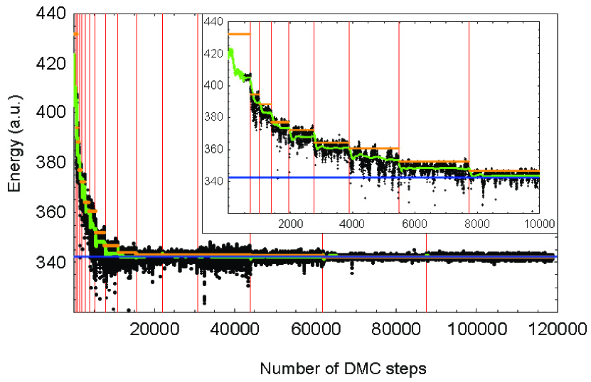
Figure 2: (Color online) Self-healed DMC run obtained using the method described in Section III. Black points denote the average value of the local energy for each DMC step. Green points mark the reference energy used for population control. Orange lines mark the average energy of the trial wave-function. The horizontal blue line marks the energy of the ground state in the full CI calculation. Vertical lines mark the steps when the coefficients of wave-function are updated. Inset: Detail of the DMC run for the first 10000 steps (same conventions as in the main figure).

From the full CI calculation we obtain a nearly exact expression of the ground state $\Psi({\bf R})=\sum_{n}a_{n}\Phi_{n}({\bf R})$.

V.2 Projection of the DMC fixed-node wave-function on a multi-determinant expansion

In order to facilitate the comparison with the full CI results, we sample the mixed-estimator density with the projectors $\xi_{n}({\bf R})$ constructed using the same basis functions of the CI expansion. For the same reason, we utilized no Jastrow function ($J=0$ in Eq. 16).

An initial trial wave-function must be selected. While the non-interacting solution has very good nodes,rosetta we intentionally chose a poor initial trial wave-function in order to test the strength of the multi-determinant method described in Section III. The worst case scenario is when the trial wave-function is orthogonal to the exact ground state. If the exact ground state is not included in the trial wave-function, a projector method such as the standard DMC algorithm cannot yield the exact ground-state energy. Accordingly, to test the method, we chose for this example $\lambda_{1}=a_{3}$, $\lambda_{3}=-a_{1}$ and $\lambda_{n}=0$ for all remaining $n$.basisnote Expanding, $\Psi_{FN}({\bf R})$ with these $\lambda_{n}$ and replacing it in Eq. (16) we obtain the projectors $\xi_{n}({\bf R})$. Next we obtained new values $\lambda_{n}$ sampling Eq. (18) every autocorrelation time. After many configurations are sampled, we construct a new trial wave-function with the new $\lambda_{n}$. We only include in the wave-function the coefficients that satisfied the condition $|\bar{\lambda}_{n}|>4\frac{\langle\tilde{\sigma}_{n}\rangle}{\sqrt{N_{c}-1}}$, i.e. that the coefficients are well determined according to this empirical threshold. Note that because the multi-determinants are solutions of a non-interacting problem, they will tend to have more nodes as their energy increases. Accordingly, high energy components of the wave-function will have smaller coefficients (${\lambda}_{n}$) in absolute value as compared with the error ($\tilde{\sigma}_{n}$). As a consequence, this acceptance threshold removes the contribution of the high energy components which implies that the resulting wave-function will be smoother than $\Psi_{FN}({\bf R})$ without the kinks at the nodes. This process is the core of a more complex algorithm we propose for larger systems that is explained in Section VI (see steps 3 and 4).

The result of this iterative approach is summarized in Figs. 2, 3, 4 and 5. In Fig. 2 we show the average of the local energy $E_{L}$ (black dots) and the best estimator for the energy $E_{best}$ (green dots)umrigar93 as a function of the number of DMC steps. The average energy of the trial wave-function $\bar{E}=\langle\Psi_{T}|H|\Psi_{T}\rangle/\langle\Psi_{T}|\Psi_{T}\rangle$ (orange) is also given for comparison. The run was carried out for a targeted population of $200$ walkers. The exact full CI result is given by the blue line. There is a dramatic decrease of $E_{L}$, $E_{best}$ and $\bar{E}$ as the trial wave-function is updated, and all these values converge to the full CI result. Similar results are obtained with different starting points and interaction strengths. The only limiting factor to reaching the exact CI results appears to be the iteration time. The reduction in the energy variance can be seen in Fig. 2 where the fluctuations in the local energy decrease as the run continues.

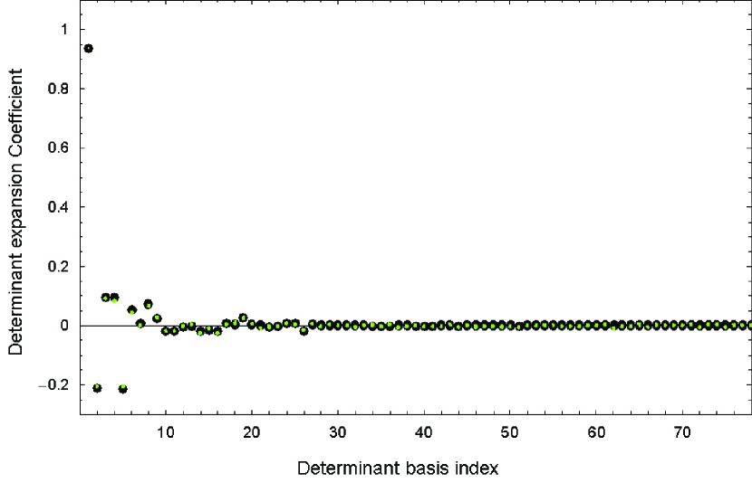
Figure 3: (Color online) Values of the coefficients of the multi-determinant expansion (small green circles) as compared with a full CI calculation (large black circles). The DMC statistical errors of the coefficients is equal to the radius of the green circles.

In Fig. 3 we show a plot of the values of the full CI coefficients as a function of the coefficient index compared with the average values obtained from the optimized trial wave-function and a final DMC run using Eq. (18). The coefficients are ordered with increasing non-interacting energy. The error bars of the coefficient are also given. The figure shows that a wave-function expansion with the quality of a CI expansion can be obtained with DMC. Note that (i) knowledge of the ground-state wave-function allows for the calculation of any other observable with an error bar that can be obtained from the error bars of the expansion coefficients. (ii) The same wave-function could be expressed with a smaller number of determinants if a Jastrow factor had been used.

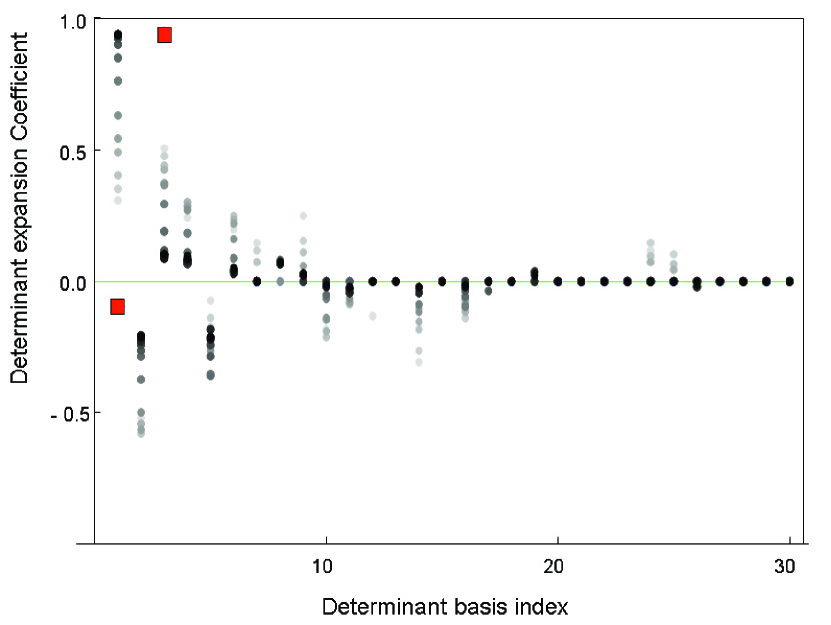
Figure 4: (Color online) Change in the values of the multi-determinant expansion as the DMC self-healing algorithm progresses. Light gray colors denote older coefficients while darker ones denote more converged results. The initial non-zero coefficients are highlighted in red squares.

In Fig. 4 we show the evolution of the values of the full CI coefficients as a the algorithm progresses starting from a trial wave-function orthogonal to the ground state.

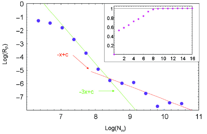
Figure 5: (Color online) Logarithm of the residual projection $R_{P}$ [see Eq. (42)] as a function of the total weighted number of configurations along the complete run $N_{w}$. The lines are a guide to the eye. Inset: projection of the DMC self-healed wave-function onto the full CI ground state as function of the logarithm of $N_{w}$.

The improved quality of the DMC optimized trial wave-function is also evident in Fig. 5. We plot the logarithm of the residual projection

$$R_{P}=\log{[1-\langle\Psi|\Psi_{T}\rangle/(|\Psi||\Psi_{T}|)]}$$ (42)

on the “exact” CI ground state as a function of the logarithm of the total weighted number of configurations along the complete run $N_{w}$. Remarkably, the error of the wave-function projection has decreased to $e^{-8}$ starting from 1. By noting that $|\Psi_{T}\rangle=|\Psi\rangle+|\delta\Psi_{\perp}\rangle$, where $|\delta\Psi_{\perp}\rangle$ is the difference between the ground-state $|\Psi\rangle$ and the trial wave function $|\Psi_{T}\rangle$ we get

$$R_{P}\simeq 2\log\left[|\delta\Psi_{\perp}|/\sqrt{2}\right]\;.$$ (43)

We can see that for a significant section of the run $R_{P}\sim 1/N_{w}^{3}$, where $N_{w}$ is the total number of weighted configurations of the run. This means that the magnitude of the error in the trial function decays with a faster exponent than $1/\sqrt{N_{w}}$ ($3/2$). This is surprising because if we had provided the exact ground state as trial wave-function, the error after finite sampling would have scaled as $|\delta\Psi_{\perp}|\sim 1/\sqrt{N_{w}}$, which replaced in Eq. (43) gives $R_{P}\simeq 1/\sqrt{N_{w}}$. This faster exponent, in a section of the plot, is a direct consequence of the fact that both the quality of the trial wave-function and the statistics have improved. This is another indication that the nodes continue to improve along the run. For the final part of the graph (the last three points), however, $R_{P}$ scales as $1/\sqrt{N_{w}}$. This possibly signals that after the nodal structure is improved to a critical distance from the exact ground state, the statistical error in the determination of the coefficients and not a small fluctuation in the nodal structure, is the limiting factor for this algorithm. We believe that a final $1/\sqrt{N_{w}}$ scaling of $R_{P}$ signals also that the overall nodal structure of the solution is correct and only small fluctuations of the coefficients are responsible for the small fluctuations from the exact node.

Since a direct sampling of the fixed-node wave-function (Eq. (18)) aims to reproduce the fixed-node solution, a single DMC run cannot improve the nodes. Only by iterating with different trial wave-functions can the nodes be improved. In particular, if an infinite number of configurations were used, the nodes would not change. In practice however, we find that for a finite sample, the error in the wave-function coefficients plays a positive role. Errors act as random fluctuations in a simulated annealing algorithm. These fluctuations are reinforcedfn:reinforced or discarded in subsequent iterations. This allows the nodal error to be systematically reduced to the point that trial wave-functions with 0.9995 projections on the full CI ground state can be found starting from a trial wave-function initially orthogonal to the ground state. Since poor nodes are associated with discontinuities in the derivative of $\Psi_{FN}({\bf R})$ at the nodal surface, and consequently an increase in the kinetic energy, it is also convenient at first to initially limit the number of configurations sampled (including first the ones that cost less non-interacting energy).

We recognize that the current work does not address the suitability and convergence of this method of relying on random fluctuations for systems with large numbers of electrons; this will be the subject of later studies.

V.3 Coulomb potential results and discussion

The use of a simplified electron-electron interaction facilitates the CI calculations and the validation of the optimization method described in Section III. However, it is also important to test the convergence and stability of the method with a realistic Coulomb interaction. Note that in two dimensions (2D) the correlations are enhanced as compared with three dimensions (3D) while the nodal surface remains non-trivial.

We tested the stability of the algorithm by replacing the interaction potential with:units $V({\bf r},{\bf r^{\prime}})=20\pi^{2}/|{\bf r-r\prime}|$. Since the length of the square box side is 1, the difference in kinetic energy between the non-interacting ground state and the first-excited state is $3\pi^{2}$. This choice of parameters for the Coulomb potential placed the system in a strongly interacting regime. To further increase the role of correlations and the difficulties that the algorithm must overcome we did not included a Jastrow term, i.e. $J=0$. We also increased the chances of failure by setting the initial trial wave-function equal to the first excited state of the non-interacting system.

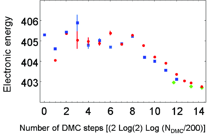
Figure 6: (Color online) Energy of the DMC run as a function of the number of DMC steps used to gather statistical data of the wave-function in the previous block. The statistical error bars for the first three points on the left were not calculated. The statistical error bars of the points on the right were smaller than the size of the symbols. Blue squares denote calculations starting from a bad trial wave-function, while the red circles mark the results obtained from an initial trial wave-function corresponding to the best blue square on the right (see text). Green diamonds were generated starting from the best red circle.

In Fig. 6 we show the evolution of the average of the local energy for each DMC optimization block as a function of the number of DMC steps in each optimization block $N_{DMC}$. Data for Eq. (18) is accumulated every $100$ DMC steps. As in the case of the model Hamiltonian, we increase $N_{DMC}$ in each optimization as $N_{DMC}=200\times 2^{n_{b}/2}$ where $n_{b}$ is the total number of blocks. With this choice we can expect the error bar in the energy and in the coefficient $\lambda_{n}$ of the multi-determinant expansion Eq. (14) to be reduced a factor $1/2$ after four successive blocks. Note that during each DMC run not only the local energy is sampled but also the values of the projectors $\xi({\bf R})$ used to construct the expansion of the trial wave-function of the next point on the right with Eq. (18).

The blue squares in Fig. 6 show the progression in average DMC energy starting from the first excited state. The initial energy is above 420 compared with the fully converged energy of 402.718 $\pm$ 0.008. Even starting from such a bad initial trial wave function, our method is able to improve in the second block after only accumulating $\approx 400$ configurations. In contrast, the red circles in Fig. 6 denote the results obtained with an initial trial wave-function constructed with data collected with the right most blue square, a very good initial trial wave-function.

As the optimization process is repeated, the average DMC energy fluctuates. Since the coefficients carry a statistical error, the wave-function is not the same from one block to the other and neither is the nodal error. There is a shift from one iteration to the next which is sometimes larger than the error bar in the energy. The energy and the variance can fluctuate and locally increase. However, as the statistics improve, fluctuations in the coefficients decrease. The statistical errors play the role of a thermal noise in the coefficient expansion. Improved statistics correspond to reduced temperatures in simulated annealing. Note that, initially, the average DMC energy from the very poor trial wave-function decreases (blue squares) as the algorithm progresses, while the energy of the average DMC energy from the good trial wave-function (red circles) actually increases. This is because when the statistics are poor the errors in the coefficient expansion allows improvement of a bad trial wave function but spoil a good quality one. Figure 6 shows that, as the algorithm progresses and improved statistics are obtained, the quality of the solution becomes independent the initial trial wave-function. Note that for intermediate blocks the DMC energy becomes flat, signaling that the the statistics are not enough to reduce the nodal error, but are sufficient to stop deterioration of the wave-function.

Repeating the algorithm iteratively leads to an incremental improvement in the statistics which results in a clear reduction of the DMC energy beyond the error bar of the preceding calculations. The DMC energy and the energy variance are reduced systematically which is a clear indication of the reduction of nodal errors and improvement in the overall quality of the wave-function. The ground-state energy obtained after 240000 accumulated DMC iterations is 402.718 $\pm$ 0.008.

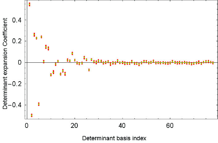
Figure 7: (Color online) Values of the coefficients of the multi-determinant expansion (small green circles) obtained from the DMC run for two electrons in a square box with a Coulomb interaction in the highly correlated limit. The statistical errors in the values of the coefficients are equal to the size of the red bar.

In Fig. 7 we show the values of the coefficients of the multi-determinant expansion as obtained with Eq. (18) corresponding to the right-most blue point in Fig. 6. Note that since no Jastrow factor is used and the interaction potential includes a singularity at ${\bf r}={\bf r^{\prime}}$, the number of coefficients with significant value is much larger the model interaction described earlier. The final reduction of nodal errors shown in the final steps of Fig. 6 is associated with subtle variations of the coefficients.

If the Jastrow factor is set to one, the density takes a simple form (Eq. (44)) in terms of the single-particle orbitals $\phi_{n}({\bf r})$. Knowledge of this density allows the calculation of the Kohn-Sham potential as explained in Ref. rosetta, (see below) and suggests an alternative route for calculation of forces by applyingpayne92 the Hellmann-Feynman theorem directly to the Kohn-Sham total energy instead of the usual statistical sampling.badinski08 ; filippi00prbr The DMC density can be obtained in terms of the single-particle orbitals with the following equation:QTS

$$\rho({\bf r})=\sum_{n,\nu}\phi_{n}^{*}({\bf r})\phi_{\nu}({\bf r})\sum_{k,l}\lambda_{k}^{*}\lambda_{l}\langle\Phi_{k}|c_{n}^{{\dagger}}c_{\nu}|\Phi_{l}\rangle\;.$$ (44)

Note in Eq. (44) that all the matrix elements $\langle\Phi_{k}|c_{n}^{{\dagger}}c_{\nu}|\Phi_{l}\rangle$ corresponding to states that differ in more than one electron hole pair, do not contribute to the ground-state density.

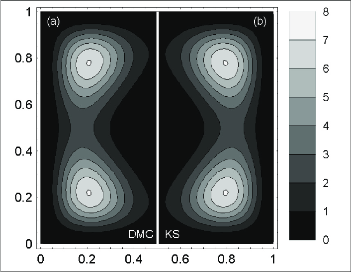
Figure 8: Density of the ground state of two spin-less electrons with Coulomb interaction in a square box. We choose one of the two degenerate ground states, reducing the symmetry of the density to $D_{2}$. a) Left side of the density of the many-body ground state constructed with the converged coefficients shown in Fig. 7. b) Kohn-Sham non-interacting density constructed as explained in Ref. rosetta, .

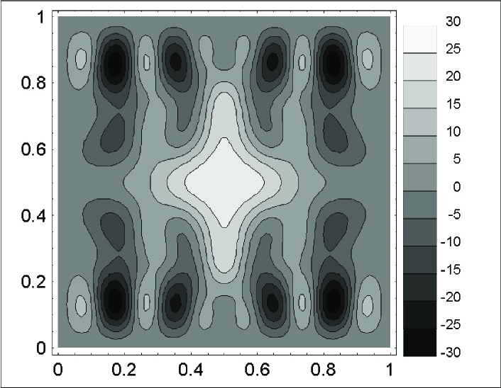
Figure 9: Kohn-Sham potential for two spin-less electrons in a square box corresponding to the ground state of Figs. 7 and 8. The potential was constructed using the methods explained in Ref. rosetta, .

In Fig. 8a we show the density corresponding to the coefficients of Fig. 7 and in Fig. 8b the non-interacting Kohn-Sham density constructed using the methods explained in Ref. rosetta, .

In Fig. 9 we show the Kohn-Sham potential obtained using the methods described in Ref. rosetta, . We minimized the cost function in Eq. (2) of Ref. rosetta, using 14 Fourier components in the potential expansion. We believe that the sampled oscillations in the Kohn-Sham potential carry some physical meaning. Indeed, these oscillations are required in order to match the non-interacting density in Fig. 8b to the interacting self-healed DMC density in Fig. 8a. However, since the density $\rho({\bf r})$ has an error $\sigma_{\rho}({\bf r})$, there is also an error in the Kohn-Sham potential. In linear response,rosetta the error bar in the potential $\sigma_{KS}({\bf r})$ (not shown) can be obtained in terms of $\sigma_{\rho}({\bf r^{\prime}})$ and the inverse susceptibility as

$$\sigma_{KS}({\bf r})=\int{\bf dr^{\prime}}\sigma_{\rho}({\bf r^{\prime}})\frac{\delta V\left({\bf r^{\prime}}\right)}{\delta\rho\left({\bf r}\right)}\;\;\;.$$ (45)

Since, we have removed degeneracies in the ground state by restricting the symmetry of the wave-function, two potentials that give the same density can only differ by a constant. We have obtained from DMC not only the approximated DMC energy but also the derivative of the total energy with respect to local fluctuations of the density. Figures 8 and 9 show that this method can provide accurate benchmarks for the validation of DFT approximations in the highly correlated regime.

V.4 Model system effective nodal potential and Jastrow factor

To demonstrate that the effective nodal potential and Jastrow factor can be obtained through sampling in DMC, in this section we determine these quantities for a model corresponding to two electrons in a square box with Coulomb interactions. An additional goal is to show that a complex (multi-determinant) wave-function can potentially be replaced by a simpler one while retaining the same nodal structure.

The results below correspond to a trial wave-function represented using the multi-determinant expansion shown in Fig. 7. While for larger dimensional systems the integrals can be performed more efficiently using a stochastic approach, in this case the probability densities were binned numerically over a grid of fifteen bins in all four dimensions. Approximately, $7.2\times 10^{5}$ weightedweighnote configurations were collected.

The one-body and two-body Jastrow factors were simply written as a Fourier expansion and their coefficients were minimized with an accelerated steepest decent algorithm using Eq. (38). The antisymmetric part of the wave-function was given by a single determinant corresponding to the ground-state solution of a non-interacting effective potential. The effective interactive potential was expressed as a sum of cosine functions and optimized as explained in Ref. rosetta, . The Jastrow factors and the potentials can be optimized at the same time. However, since we wanted the Jastrow factor to carry most of the load in the optimization of the symmetric corrections to the probability density, the potential was optimized only every third iteration that the Jastrow factor was optimized.

The resulting potential, and Jastrow factors are shown in Fig. 10. The value of the cost-function was reduced an order of magnitude from starting with the non-interacting ground state with zero effective potential. The effective potential resulting from this minimization procedure is an example of the nodal potential predicted in Ref. rosetta, .

We also performed tests of this optimization algorithm using the model interaction discussed in Subsection V.2. In this case the nodal structure of the wave-function was also improved (as signaled by a reduction of the average DMC energy below the error bar of the preceding calculation).

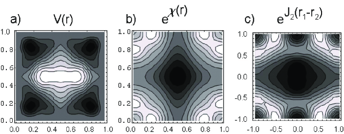
Figure 10: a) Effective nodal potential, b) one-body Jastrow, and c) two-body Jastrow factors obtained by minimizing Eq. (29), in which the multi-determinant expansion of Fig. 7 has been replaced by a single determinant function.

VI Summary of improved self-healing DMC algorithm

It is clear from previous sections that an effective wave-function optimization algorithm can be constructed solely on the basis of iteratively updating $\Psi_{T}$ by the multi-determinant expansion of $\Psi_{FN}$. An example of this algorithm applied to a soluble model is presented in Subsection V.2. However, multi-determinant expansions in DMC are computationally very expensive in large or continuum system, since the required number of determinants to reach a given accuracy will in general grow combinatorially. The method developed in Section IV to optimize a single Slater determinant becomes very attractive. (Results of the application of this method were shown in Subsection V.4). For large systems, the number of multi-determinants must be kept to a minimum and the two methods combined. Experimentation in small systems allows us to suggest an algorithm that will be efficient in larger systems:

1. An initial trial trial wave-function $\Phi_{T}({\bf R})$ is generated using any fast method, e.g. an empirical screened pseudopotentialwang95 or a Thomas-Fermi theory.

2. The Jastrow factor $J({\bf R})$ is optimized within VMC.

3. A DMC run is performed. The number of configurations $N_{c}$ sampled is increased as this step is repeated. Statistically uncorrelated values of $\xi_{n}({\bf R})$ and $\xi_{n}({\bf R})^{2}$ are accumulated.

4. The multi-determinant expansion of $f({\bf R})$ is constructed. Only the terms that are significantly non-zero are included in the expansion.

5. A distribution of configurations ${\bf R}_{i}$ with probability $|W({\bf R})|$ is generated. The gradients of $K_{DMC}$ with respect to the effective nodal potential and the gradients of the Jastrow factor coefficients are evaluated with Eqs. (36), and (41). (Eventually the multi-determinant expansion coefficients $\alpha_{k}$ can be included, see Subsection IV.6.)

6. The effective potentials $V\left({\bf r}\right)$ and $\tilde{J}({\bf R})$ are updated (eventually also the $\alpha_{k}$). New single particle orbitals are constructed using Eq. (31). Therefore the single particle orbitals used to construct the Slater determinants in the trial wave-function are now determined solely within DMC.

7. A new $\tilde{\Psi}_{T}({\bf R})$ is constructed. Steps (5-7) are repeated until $\tilde{\Psi}_{T}({\bf R})$ does not change.

8. At this step we can choose to improve the scaling in large systems. The single-particle orbitals $\phi_{n}({\bf r})$ shared by all determinants in the expansion $\tilde{\Phi}_{T}({\bf R})$ can be transformed to non-orthogonal localized orbitals.reboredo05 ; alfe04

9. The trial wave-function $\Phi_{T}({\bf R})$ is updated to $\tilde{\Phi}_{T}({\bf R})$. Steps (2-9) are repeated until $\tilde{\Psi}_{T}({\bf R})$ and $E_{DMC}$ do not change.fn:change

Note that (i) the methods in Sections III and IV are complementary. In Section III, we find a representation of the fixed-node ground state in a given basis. In Section IV, instead, we optimize and change the basis of the wave-functions so as to reproduce the fixed-node ground-state wave-function with a minimum number of Slater determinants. (ii) Only single configurations are included in Eq. (36) but multiple configurations are included in Eq. (14). (iii) We include a Jastrow function in Eq. (14) to minimize the number of Slater determinants required in the expansion. However, a final run with no Jastrow factor included with the configuration interaction expansion might be useful in order to obtain a pure expression of the ground-state density in terms of the single particle orbitals. Atomic forces could be obtained from this density. Finally (iv) the method is, in principle, self reliant: no DFT or HF are required.

VII Summary

We have presented an algorithm for sampling the fixed-node many-body wave-function in a single or multi-determinant expansion from a diffusion quantum Monte Carlo (DMC) calculation within the importance sampling technique. By combining this algorithm with a previously developed method for constructing effective potentials targeted at reproducing specific properties of the many-body wave-function,rosetta we presented an iterative algorithm that improves the nodes of the trial/fixed-node wave-functions used in DMC. Tests on a simple two electron model system confirm that this method is able to improve the nodes and that, at least in the case of the tested system, we find wave-functions and energies that exactly match fully converged configuration interaction calculations.

We have proven that the nodes of the fixed-node wave-function improve as compared with the trial wave-function if the kinks at the nodes are locally smoothed out. The algorithms presented take advantage of this proof. We have argued that if the kink at the node increases with the “distance” from the exact ground-state node to the trial wave-function node, the algorithm should be stable against random statistical fluctuations. Proving this property in general might be difficult and is beyond the scope of this article. Clearly, in the absence of a proof, experimentation in larger systems is required.

While in the past, methods were used to obtain the fixed-node wave-function (e.g Ref. bianchi96, ), to our knowledge this is the first time the fixed-node wave-function has been obtained through importance sampling. The availability of the fixed-node wave-function provides routes to determine the exact Kohn-Sham potential, allowing benchmark tests of density functionals in highly non-trivial and inhomogeneous systems. It also seems likely that many of the wave function optimization approaches (e.g. Refs. filippi00, ; umrigar07, ; rios06, ; luchow07, ) currently applied within variational Monte Carlo can be recast in the present scheme, making direct use of the fixed-node wave-function, and likely obtaining improved results.

In ongoing work, we are continuing to develop these methods. Applications to larger and more complex electronic systems will be reported elsewhere.

References

- (1) J. B. Anderson, Int. J. of Quantum Chem. 15, 109 (1979).
- (2) D. M. Ceperley and B. J. Alder, Phys. Rev. Lett. 45, 566 (1980).
- (3) The energy of any wave-function being for a given Hamiltonian .
- (4) P. J. Reynolds, D. M. Ceperley, B. J. Alder, and W. A. Lester, J. Chem. Phys. 77, 5593 (1982).
- (5) M. Bajdich, L. Mitas, G. Drobny, and L. K. Wagner, Phys. Rev. B 72, 075131 (2005); L. Mitas, Phys. Rev. Lett. 96, 240402 (2006).
- (6) C. Filippi and S. Fahy, J. Chem. Phys. 112, 3523 (2000).
- (7) C. J. Umrigar, J. Toulouse, C. Filippi, S. Sorella, and R. G. Hennig, Phys. Rev. Lett. 98, 110201 (2007).
- (8) P. Lòpez-Rios, A. Ma, N. D. Drummond, M. D. Towler, and R. J. Needs, Phys. Rev. E 74, 066701 (2006).
- (9) A. Lüchow, et. al., J. Chem. Phys. 126, 144110 (2007).
- (10) M. H. Kalos and F. Pederiva, Phys Rev. Lett. 85, 3547 (2000).
- (11) D. M. Ceperley and B. J. Alder, J. Chem. Phys. 81, 5833 (1984).
- (12) S. W. Zhang and M. H. Kalos, Phys. Rev. Lett. 67, 3074 (1991).
- (13) T. D. Beaudet, M. Casula, J. Kim, S. Sorella, and R. M. Martin, J. Chem. Phys. 129, 164711 (2008).
- (14) J. Toulouse and C. J. Umrigar, J. Chem. Phys. 128, 174101 (2008).
- (15) A. J. Williamson, R. Q. Hood, and J. C. Grossman, Phys. Rev. Lett. 87, 246406 (2001).
- (16) F. A. Reboredo and A. J. Williamson, Phys. Rev. B 71, 121105(R) (2005).
- (17) D. Alfe and M. J. Gillan, Phys. Rev. B 70, 161101(R) (2004).
- (18) F. A. Reboredo and P. R. C. Kent, Phys. Rev. B. 77, 245110 (2008).
- (19) M. L. Tiago, P. R. C. Kent, R. Q. Hood, and F. A. Reboredo, J. Chem. Phys. 129, 084311 (2008).
- (20) B. L. Hammond, W. A. Lester, Jr., and P. J. Reynolds Monte Carlo Methods in Ab Inition Quantum Chemistry (World Scientific, Singapore-New Jersey-London-Hong Kong, 1994).
- (21) S. Vitiello, K. Runge, and M. H. Kalos, Phys. Rev. Lett. 60, 1970 (1988).
- (22) Equation (II) can be thought of as a one-step ( in Eq. (3)) in a pure-diffusion DMC run using the small propagator of Eq. (4), in which the positive and negative walkers have the initial distribution and are not constrained by the nodes of .
- (23) Because of elemental group theory theorems, i) the product of two anti-symmetric functions is symmetric, ii) the product of any symmetric operator with any anti-symmetric function results in an anti-symmetric function (with no projection on any symmetric bosonic function or any other representation of the symmetric group). Thus our analytic derivation is true. Since we use an anti-symmetric representation of the wave-function, our numerical method will not find bosonic states since they are excluded from the search.bianchi93
- (24) The nodes continue to move statistically in the same direction in successive iterations.
- (25) The “release-node” method ceperley80 ; HLRbook involves two fixed trial wave-functions and two populations of walkers. Our method is very different since, instead, involves only one trial wave-function that is updated and a single population of walkers. In our method the walkers never cross the node: we move the node instead. In the so called release-node method the node is removed.
- (26) R. Bianchi, D. Bressanini, P. Cremaschi, M. Mella, and G. Morosi, J. Chem. Phys. 98, 7204 (1993).
- (27) R. Bianchi, D. Bressanini, P. Cremaschi, M. Mella, and G. Morosi, Int. J. of. Quant. Chem. 57, 321 (1996).
- (28) F. A. Reboredo and C. R. Proetto, Phys. Rev. B 67, 115325 (2003).
- (29) In Ref. us, the projectors are denoted as .
- (30) C. J. Umrigar, M. P. Nightingale, and K. J. Runge, J. Chem. Phys. 99, 2865 (1993).
- (31) B. Wood and W. M. C. Foulkes, J. of Phys. C 18, 2305 (2006).
- (32) A. A. Correa, F. A. Reboredo, and C. A. Balseiro, Phys. Rev. B 71, 035418 (2005).
- (33) P. Hohenberg and W. Kohn, Phys. Rev. 136, B864 (1964).
- (34) R. G. Parr and W. Yang, Density-Functional Theory of Atoms and Molecules (Oxford Science Publications, Oxford, 1989).
- (35) W. Kohn and L. J. Sham, Phys. Rev. 140, A1133 (1965).
- (36) In section V.4 we solve a case where it is more efficient to bin .
- (37) We define the energy unit to be .
- (38) The basis functions in the CI expansion are ordered with increasing non-interacting energy.
- (39) M.C. Payne, M.P. Teter, D.C. Allan, T.A. Arias, and J.D. Joannopoulos Rev. Mod. Phys. 64, 1045 (1992).
- (40) A. Badinski and R. J. Needs, Phys. Rev. B 78, 035134 (2008).
- (41) C. Filippi and C. J. Umrigar, Phys. Rev. B 61, R16291 (2000).
- (42) C. Kittel Quantum Theory of Solids (John Wiley & Sons, New York, 1987).
- (43) The weight of the walkers goes from 2 to 1/2 and is multiplied by the correction given in Eq. (19).
- (44) L.-W. Wang and A. Zunger, Phys. Rev. B 51, 17398 (1995).
- (45) must be converged twice: first in order to fit the fixed-node solution which allows the node to move, and second when the node no longer moves.