Call option prices based on Bessel processes

Abstract.

As a complement to some recent work by Pal and Protter [9], we show that the call option prices associated with the Bessel strict local martingales are integrable over time, and we discuss the probability densities obtained thus.

1. Introduction: some general remarks

1.1.

Let $(M_{t},t\geq 0)$ denote a continuous local martingale, taking values in $\mathbb{R}_{+}$. To any $K>0$, we associate the process $(K-M_{t})^{+},\ t\geq 0$. It is not difficult to show, after localizing $M$, that this process $(K-M_{t})^{+}$ is a (bounded) submartingale, and, as a consequence, the function:

$$m_{K}^{(+)}(t)=E\big{[}\left(K-M_{t}\right)^{+}\big{]},\ t\geq 0$$

is increasing, and bounded (by $K$). The study of such functions, considered (essentially) as distribution functions, has been the subject of the Bachelier Course [1, 2], given by the second author. In particular, if $M_{t}\underset{t\rightarrow\infty}{\rightarrow}0$, there is the formula

$$E\left[F_{t}\left(K-M_{t}\right)^{+}\right]=KE\left[F_{t}1_{(\mathcal{G}_{K}\leq t)}\right]$$ (1)

which is valid for every $F_{t}\geq 0$, $(\mathcal{F}_{t})$ measurable, and $\mathcal{G}_{K}=\sup\left\{t:M_{t}=K\right\}$. See also Madan-Roynette-Yor [6, 7, 8].

1.2.

The present paper is devoted to the study of the functions:

$$m_{K}^{(-)}(t)=E\big{[}\left(M_{t}-K\right)^{+}\big{]}=E\big{[}\left(K-M_{t}\right)^{-}\big{]},\ t\geq 0,$$

which play an important role in option pricing, as $(m_{K}^{(-)}(t))$ is the European call price with strike $K$, and maturity $t$, associated with the local martingale $(M_{t})$. If $(M_{t})$ is a ”true” martingale, then $\{(M_{t}-K)^{+}\}$ is a submartingale, hence $(m_{K}^{(-)}(t),t\geq 0)$ is increasing. On the other hand, if $(M_{t},t\geq 0)$ is a strict local martingale, that is: a local martingale, which is not a martingale, then the function $(m_{K}^{(-)})$ is not in general increasing, or even monotone.

1.3.

The most well-known example of a strict local martingale is $M_{t}=1/R_{t}$, where $(R_{t},t\geq 0)$ denotes the $BES(3)$ process, starting from 1, or, by scaling, equivalently from any $r>0$. Then, the study of $(m_{K}^{(-)}(t))$ in this particular case has been undertaken in a remarkable paper by S. Pal and P. Protter [9]; the results of which have strongly motivated the present paper.

In the present paper, we take up again the study of this function $(m_{K}^{(-)}(t))$ in this particular case; we show that:

$$\int_{0}^{\infty}dt\ m_{K}^{(-)}(t)<\infty.$$

Hence, up to a multiplicative constant $(m_{K}^{(-)}(t),\ t\geq 0)$ is a probability density on $\mathbb{R}_{+}$; we identify the Laplace transform of this probability, and describe it as the law of a certain random variable defined uniquely in terms of $BES(3)$ process. This is done thanks to the Doob $h$-transform understanding of $BES(3)$ (from Brownian motion, killed when hitting 0), combined with general identity (1). We refer the reader to Section 2 for precise statements. In Section 3, we develop the same kind of study but this time with $M_{t}=1/R_{t}^{(\delta-2)},\ t\geq 0$, where $(R_{t},\ t\geq 0)$ denotes the $BES(\delta)$ process, starting from 1. In Section 4, we present the graphs of the corresponding functions $(m_{K}^{(-)}(t),\ t\geq 0)$.

1.4.

To summarize, the main point of this work is to use the interpretation of the generalized Black-Scholes quantities in terms of last passage times (formula (1)) in the framework of Bessel processes in order to derive fine properties of the call option process, as a function of maturity, written for the strict local Bessel martingales.

2. Some results about $r_{K}^{(3)}(t)\equiv E_{1}^{(3)}\big{[}\big{(}\frac{1}{X_{t}}-K\big{)}^{+}\big{]},\ t\geq 0$

2.1.

In this section, we change notation slightly: $(X_{t},\ t\geq 0)$ denotes the canonical process on $C(\mathbb{R}_{+},\mathbb{R}_{+})$, $W_{x}$ is Wiener measure such that $W_{x}(X_{0}=x)=1$, and $P_{x}^{(3)}$ is the law of the $BES(3)$ process starting from $x$. In fact, we shall only consider $x=1$ (except mentioned otherwise).

2.2.

Here are our 3 main results concerning the functions $r_{K}^{(3)}(t)$.

Proposition 1.

The following holds:

• $(t\rightarrow\infty)$: $r_{0}^{(3)}(t)\sim\sqrt{\frac{2}{\pi t}};\ \ r_{K}^{(3)}(t)\sim\frac{1}{3\sqrt{2\pi}t^{3/2}K^{2}}$

• $(t\rightarrow 0)$: $r_{K}^{(3)}(t)\rightarrow(1-K)^{+}$; $r_{1}^{(3)}(t)\sim\sqrt{\frac{t}{2\pi}}$.

An important consequence of Proposition 1, (i), is that, for $K>0$, the function $(r_{K}^{(3)}(t),t\geq 0)$ is integrable over $\mathbb{R}_{+}$, hence it is, up to a multiplicative constant, a density of probability on $\mathbb{R}_{+}$. We now describe this probability.

Proposition 2.

• The function $(3K^{2}r_{K}^{(3)}(t),t\geq 0)$ is a probability density on $\mathbb{R}_{+}$.

• It is the density of

  $$\Lambda_{K}^{(3)}\stackrel{{\scriptstyle\rm{(law)}}}{{=}}(g_{1}-\widetilde{T}_{k})+\widetilde{T}_{k}U$$ (2)

  where, on the RHS of (2), $k=1/K$, the variables $g_{1}$, $\widetilde{T}_{k}$, and $U$ are independent, $g_{1}=\sup\{t:X_{t}=1\}$, $\widetilde{T}_{k}$ is the size-biased sampling of $T_{k}=\inf\{t:X_{t}=k\}$, with $g_{1}$ and $T_{k}$ defined with respect to $P_{0}^{(3)}$, and finally $U$ is uniform on $[0,1]$.

As a further description of the law of $\Lambda_{K}^{(3)}$, we present its Laplace transform.

Proposition 3.

The Laplace transform of $\Lambda_{K}^{(3)}is$: (we use again $k=1/K$)

$$E\left[\exp(-\lambda\Lambda_{K}^{(3)})\right]=\frac{3}{\lambda k^{2}}\left(e^{-\sqrt{2\lambda}}\right)\left(\frac{\sinh(\sqrt{2\lambda}k)}{\sqrt{2\lambda}k}-1\right)$$

2.3. Proofs of Propositions 1, 2, 3

2.3.1.

The main ingredients of these proofs are the following:

• the Doob $h$-process relationship between Brownian motion and $BES(3)$, which may be written as:

  $$P_{1}^{(3)}|_{\mathcal{F}_{t}}=\left(X_{t\wedge T_{0}}\right)\cdot W_{1}|_{\mathcal{F}_{t}}$$

• the particular instance of formula (1) with $M_{t}=X_{t\wedge T_{0}}$, under $W_{1}$:

  $$W_{1}\left(F_{t}\left(k-X_{t\wedge T_{0}}\right)^{+}\right)=kW_{1}\left(F_{t}1_{(\gamma_{k}\leq t)}\right)$$

  with $\gamma_{k}=\sup\{t<T_{0}:X_{t}=k\}$.

• the time reversal result: $(X_{T_{0}-t},\ t\leq T_{0})$ under $W_{1}$ is distributed as
  $(X_{t},\ t\leq g_{1})$ under $P_{0}^{(3)}$.

2.3.2.

Thanks to the preceding points, we may now obtain interesting description of $r_{K}^{(3)}(t)$ in terms of first and last passage times. In fact, we obtain:

$$r_{K}^{(3)}(t)=W_{1}\left(\gamma_{k}<t<T_{0}\right)$$ (3)

or, equivalently, from the time reversal result in (iii):

$$r_{K}^{(3)}(t)=P_{0}^{(3)}(g_{1}>t)-P_{k}^{(3)}(g_{1}>t).$$ (4)

Proof of (3):
Combining (i) and (ii) above, we obtain:

$$r_{K}^{(3)}(t) = W_{1}\left(\left(1-KX_{t}\right)^{+}1_{(t<T_{0})}\right)$$

$$= KW_{1}\left(\left(k-X_{t\wedge T_{0}}\right)^{+}1_{(t<T_{0})}\right),\ \ \mbox{with }k=\frac{1}{K}$$

$$= KkW_{1}\left(\gamma_{k}\leq t<T_{0}\right)$$

$$\equiv W_{1}\left(\gamma_{k}<t<T_{0}\right),\ \ \mbox{which is }(\ref{r_K3_W1}).$$

2.3.3.

Proof of Proposition 2:

• We deduce from (3) that:

  $$\int_{0}^{\infty}dt\ r_{K}^{(3)}(t)=W_{1}\left(T_{0}-\gamma_{k}\right)=E_{0}^{(3)}(T_{k}),$$

  by time reversal. Using the fact that $(R_{t}^{2}-3t,t\geq 0)$ is a $P_{0}^{(3)}$-martingale, we get:

  $$3E_{0}^{(3)}(T_{k})=k^{2}.$$

  Hence, the constant $c$ we were seeking is: $c=\frac{3}{k^{2}}$, and $\frac{3}{k^{2}}r_{K}^{(3)}(t)\equiv 3K^{2}r_{K}^{(3)}(t)$ is a probability density on $\mathbb{R}_{+}$.

• In order to identify a random variable $\Lambda_{K}^{(3)}$ with distribution $3K^{2}r_{K}^{(3)}(t)$, we go back to (3) and we get, for any $f:\mathbb{R}_{+}\rightarrow\mathbb{R}_{+}$, Borel:

  $$\int_{0}^{\infty}dt\ f(t)\ 3K^{2}r_{K}^{(3)}(t)=3K^{2}W_{1}\left(\int_{\gamma_{k}}^{T_{0}}dt\ f(t)\right)$$

  $$=3K^{2}W_{1}\left[f\left(\gamma_{k}+\left(T_{0}-\gamma_{k}\right)U\right)\left(T_{0}-\gamma_{k}\right)\right]$$

  $$=3K^{2}E_{0}^{(3)}\left[f\left(\left(g_{1}-T_{k}\right)+T_{k}U\right)T_{k}\right],$$

  where $U$ is uniform on $[0,1]$, independent of $T_{k}$ and $g_{1}$. Hence using the notation of $\widetilde{T}_{k}$ for the size-biased sampling of $T_{k}$, we get that:

  $$E\left(f\left(\Lambda_{K}^{(3)}\right)\right)=E_{0}^{(3)}\left[f\left(\left(g_{1}-\widetilde{T}_{k}\right)+\widetilde{T}_{k}U\right)\right].$$

$\Box$

2.3.4.

Proof of Proposition 3:
From formula (3) again, this Laplace transform is:

$$3K^{2}W_{1}\left(\int_{\gamma_{k}}^{T_{0}}dt\ e^{-\lambda t}\right)=\frac{3K^{2}}{\lambda}W_{1}\left(e^{-\lambda\gamma_{k}}-e^{-\lambda T_{0}}\right).$$

The result now follows from:

$$W_{1}\left(e^{-\lambda T_{0}}\right)=e^{-\sqrt{2\lambda}}=W_{1}\left(e^{-\lambda\gamma_{k}}\right)\frac{\sqrt{2\lambda}k}{\sinh(\sqrt{2\lambda}k)}.$$

$\Box$

2.3.5.

Proof of Proposition 1:

• As $t\rightarrow\infty$, we have:

  $$r_{0}^{(3)}(t) = E_{1}^{(3)}\left(\frac{1}{R_{t}}\right)=\frac{1}{\sqrt{t}}\ E_{(1/\sqrt{t})}^{(3)}\left(\frac{1}{R_{1}}\right)$$

  $$\underset{t\rightarrow\infty}{\sim} \frac{1}{\sqrt{t}}\ E_{0}^{(3)}\left(\frac{1}{R_{1}}\right)=\sqrt{\frac{2}{\pi t}}.$$

  The equivalent, for $K>0$, of $r_{K}^{(3)}(t)$, as $t\rightarrow\infty$, is simply the particular case: $\delta=3$ of the result in (i) of Proposition 4.

• The first statement follows from the convergence in $L^{1}$ of $\frac{1}{X_{t}}$ to 1 as $t\rightarrow 0$; For the second statement, we use:

  $$r_{1}^{(3)}(t) = W_{1}\left(\left(1-X_{t}\right)^{+}1_{(t<T_{0})}\right)$$

  $$= W_{1}\left(\left(1-X_{t}\right)^{+}\right)-W_{1}\left(\left(1-X_{t}\right)^{+}1_{(T_{0}<t)}\right).$$

  The first term is: $W_{0}(X_{t}^{+})=\sqrt{\frac{t}{2\pi}}$, whereas the second one may be majorized by

  $$W_{1}\left(T_{0}<t\right) = W_{0}\left(T_{1}<t\right)=W_{0}\left(|X_{1}|>\frac{1}{\sqrt{t}}\right)$$

  $$= \sqrt{\frac{2}{\pi}}\int_{1/\sqrt{t}}^{\infty}du\ e^{-(u^{2}/2)}\leq e^{-1/2t}$$

(Note that, in fact, it is not necessary to use Proposition 1 to obtain Propositions 2 and 3; however, it is the result of Proposition 1, (i), which led us to study $\Lambda_{K}^{(3)}$).

2.3.6.

A more direct proof of the estimate: $r_{K}^{(3)}(t)=\mathrm{O}\left(\frac{1}{t^{3/2}}\right)$, as $t\rightarrow\infty$.
Since this estimate plays quite some role in our paper, it seems of some interest to look for a simple proof of it. We note that:

$$r_{K}^{(3)}(t)\equiv E_{1}^{(3)}\left(\left(\frac{1}{R_{t}}-K\right)^{+}\right)\leq E_{0}^{(3)}\left(\left(\frac{1}{R_{t}}-K\right)^{+}\right)$$

since, from the additivity property of squares of Bessel processes (Shiga-Watanabe [14]), a Bessel process with dimension $\delta$, starting from $a>0$, dominates stochastically a Bessel process with dimension $\delta$, starting from 0. Now we have:

$$E_{0}^{(3)}\left[\left(\frac{1}{R_{t}}-K\right)^{+}\right]$$

$$= E_{0}^{(3)}\left[\left(\frac{1}{\sqrt{t}{R_{1}}}-K\right)^{+}\right]\ \ \ \ \mbox{(by scaling)}$$

$$= c\int_{0}^{1/\sqrt{t}K}dr\ r^{2}e^{-r^{2}/2}\left(\frac{1}{\sqrt{t}r}-K\right),\ \ \ \mbox{for some universal constant c}$$

$$\leq \frac{c}{\sqrt{t}}\int_{0}^{1/\sqrt{t}K}dr\ re^{-r^{2}/2}$$

$$= \frac{c}{\sqrt{t}}\left(1-\exp\left(-\frac{1}{2tK^{2}}\right)\right)\underset{t\rightarrow\infty}{\sim}\frac{c}{2t^{3/2}K^{2}}.$$

3. Extending the previous results to: $r_{K}^{(\delta)}(t)\equiv E_{1}^{(\delta)}\big{[}\big{(}\frac{1}{R_{t}^{\delta-2}}-K\big{)}^{+}\big{]},\ \delta>2$

3.1.

In this section, $(X_{t},\ t\geq 0)$ still denotes the canonical process on $C(\mathbb{R}_{+},\mathbb{R}_{+})$, and we consider $P_{x}^{(\delta)}$ the law of the $BES(\delta)$ process, starting from $x$ (which, again, will be taken mainly equal to 1).

3.2.

As a parallel to Section 2, we offer 3 results concerning the function $r_{K}^{(\delta)}$. We note $\nu=\frac{\delta}{2}-1$

Proposition 4.

The following holds:

• $(t\rightarrow\infty)$: $r_{0}^{(\delta)}(t)\sim\frac{1}{t^{\nu}2^{\nu}\Gamma(1+\nu)};\ \ r_{K}^{(\delta)}(t)\sim\frac{C_{K}^{(\delta)}}{t^{\nu+1}},\ \mbox{with }C_{K}^{(\delta)}=\frac{1}{2^{\nu+1}(\nu+1)\Gamma(\nu)K^{(1/\nu)}}$

• $(t\rightarrow 0)$: $r_{K}^{(\delta)}(t)\rightarrow(1-K)^{+}$; $r_{1}^{(\delta)}(t)\sim\sqrt{t}(2\nu)\frac{1}{\sqrt{2\pi}}$

Proposition 5.

• The function $\left(\delta K^{2/(\delta-2)}r_{K}^{(\delta)}(t),t\geq 0\right)$ is a probability density on $\mathbb{R}_{+}$.

• It is the density of

  $$\Lambda_{K}^{(\delta)}\stackrel{{\scriptstyle\rm{(law)}}}{{=}}\left(g_{1}-\widetilde{T}_{k}\right)+\widetilde{T}_{k}U$$ (5)

  where, on the RHS of (5), $k=1/K^{1/(\delta-2)}$, the variables $g_{1}$, $\widetilde{T}_{k}$, and $U$ are independent, $g_{1}=\sup\{t:X_{t}=1\}$, $\widetilde{T}_{k}$ is the size-biased sampling of $T_{k}=\inf\{t:X_{t}=k\}$, with $g_{1}$ and $T_{k}$ defined with respect to $P_{0}^{(\delta)}$, and finally $U$ is uniform on $[0,1]$.

Finally, we present the Laplace transform of $\Lambda_{K}^{(\delta)}$.

Proposition 6.

The Laplace transform of $\Lambda_{K}^{(\delta)}$ is:

$$E\left[\exp(-\lambda\Lambda_{K}^{(\delta)})\right]=\frac{2\delta K^{2/(\delta-2)}}{\lambda}\left(\mathcal{K}_{\nu}(\sqrt{2\lambda})\right)\left\{\frac{\nu I_{\nu}(k\sqrt{2\lambda})}{k^{\nu}}-\frac{1}{\Gamma(\nu)}\left(\frac{\sqrt{2\lambda}}{2}\right)^{\nu}\right\}$$

where $I_{\nu}$ and $\mathcal{K}_{\nu}$ denote the usual modified Bessel functions, with parameter $\nu$ (we use $\mathcal{K}_{\nu}$ instead of $K_{\nu}$ so that no confusion with the strike $K$ may occur).

3.3. Proofs of Propositions 4, 5, 6

We follow the rationale of the proofs of Propositions 1, 2, 3, after extending adequately the points (i), (ii) and (iii) in (2.3.1) from the $BES(3)$ process to $BES(\delta)$ process, for $\delta>2$.

3.3.1.

Here are these extensions:

• the Doob $h$-process relationship between $BES(\delta)$ and $BES(4-\delta)$, killed upon hitting 0, is

  $$P_{1}^{(\delta)}|_{\mathcal{F}_{t}}=\left(X_{t\wedge T_{0}}\right)^{2\nu}\cdot P_{1}^{(4-\delta)}|_{\mathcal{F}_{t}},$$

  where $\delta=2(1+\nu)$.

• the particular instance of formula (1) with $M_{t}=(X_{t\wedge T_{0}})^{2\nu}$ under $P_{1}^{(4-\delta)}$:

  $$E_{1}^{(4-\delta)}\left[F_{t}\left(C^{2\nu}-\left(X_{t\wedge T_{0}}\right)^{2\nu}\right)^{+}\right]=C^{2\nu}E_{1}^{(4-\delta)}\left[F_{t}1_{(\gamma_{{}_{C}}\leq t)}\right]$$

  with $\gamma_{{}_{C}}=\sup\left\{t<T_{0}:X_{t}=C\right\}$.

• the time reversal result:
  $(X_{(T_{0}-t)},\ t\leq T_{0})$ under $P_{1}^{(4-\delta)}$ is distributed as $(X_{t},t\leq g_{1})$ under $P_{0}^{(\delta)}$.

3.3.2.

The preceding results lead us to the following descriptions of $r_{K}^{(\delta)}(t)$ in terms of first and last passage times:

$$r_{K}^{(\delta)}(t) = P_{1}^{(4-\delta)}(\gamma_{k}\leq t\leq T_{0})\hskip 133.69994pt(3)_{\delta}$$

$$= P_{0}^{(\delta)}(g_{1}>t)-P_{k}^{(\delta)}(g_{1}>t)\hskip 104.06897pt(4)_{\delta}$$

where $k=1/K^{1/(\delta-2)}$

3.3.3.

Proof of Proposition 5:
It suffices to follow the arguments of the proof of Proposition 2, replacing everywhere dimensions 1 and 3 by dimensions $(4-\delta)$ and $\delta$.                                    $\Box$

3.3.4.

Proof of Proposition 6:
Starting from $(3)_{\delta}$ we obtain:

$$E\left[\exp\left(-\lambda\Lambda_{K}^{(\delta)}\right)\right]=\left(\frac{\delta}{k^{2}}\right)E_{1}^{(4-\delta)}\left[\int_{g_{k}}^{T_{0}}dt\ e^{-\lambda t}\right]$$

$$=\frac{\delta}{k^{2}\lambda}\left(E_{1}^{(4-\delta)}\left(e^{-\lambda g_{k}}\right)-E_{1}^{(4-\delta)}\left(e^{-\lambda T_{0}}\right)\right)$$

$$=\frac{\delta}{k^{2}\lambda}E_{1}^{(4-\delta)}\left(e^{-\lambda T_{0}}\right)\left\{\frac{1}{E_{0}^{(\delta)}\left(e^{-\lambda T_{k}}\right)}-1\right\}$$

$$=\frac{\delta}{k^{2}\lambda}E_{0}^{(\delta)}\left(e^{-\lambda g_{1}}\right)\left\{\frac{1}{E_{0}^{(\delta)}\left(e^{-\lambda T_{k}}\right)}-1\right\}$$

with the help of the time reversal result (iii)_δ. Now, classical computations of Laplace transforms for first hitting times and last passage times of Bessel processes yield (see, e.g., Kent [4], Pitman-Yor [10]):

$$E_{0}^{(\delta)}\left(e^{-\lambda g_{1}}\right) = \frac{2}{\Gamma(\nu)}\left(\frac{\sqrt{2\lambda}}{2}\right)^{\nu}\mathcal{K}_{\nu}\left(\sqrt{2\lambda}\right)$$

$$E_{0}^{(\delta)}\left(e^{-\lambda T_{k}}\right) = \frac{(\sqrt{2\lambda}k)^{\nu}}{2^{\nu}\Gamma(\nu+1)I_{\nu}(k\sqrt{2\lambda})}$$

where $\mathcal{K}_{\nu}$ and $I_{\nu}$ denote the usual modified Bessel functions with index $\nu$. Finally, we have obtained the formula given in Proposition 6.

3.3.5.

Proof of Proposition 4:
For $K=0$, the result follows by scaling, as in dimension 3.
For $K>0$,

• We shall use formula $(4)_{\delta}$ (to obtain the asymptotic result for $r_{K}^{(\delta)}(t),\ t\rightarrow\infty$) together with the formula for the distribution of a last passage time of a transient diffusion (see, e.g., Pitman-Yor [10], as well as Salminen [12, 13]):

  $$P_{x}\left(g_{y}\in dt\right)=-\frac{s^{\prime}(y)a(y)}{2s(y)}p_{t}(x,y)dt.$$

  In our present case, we have: $s(y)=-1/y^{(\delta-2)}$, so that: $-\frac{s^{\prime}(y)}{s(y)}=\frac{(\delta-2)}{y}$; $a(y)=1$. Thus we have:

  $$P_{x}^{(\delta)}(g_{y}\in dt)=\left(\frac{\delta-2}{2y}\right)p_{t}^{(\delta)}(x,y)dt,$$

  so that, going back to the expression $(4)_{\delta}$ for $r_{K}^{(\delta)}$, we get:

  $$r_{K}^{(\delta)}(t)=\frac{\delta-2}{2}\int_{t}^{\infty}ds\ \left(p_{s}^{(\delta)}(0,1)-p_{s}^{(\delta)}(k,1)\right).$$ (6)

  Next, we shall use the following explicit formulae: (with $\nu=\frac{\delta-2}{2}$)

  $$p_{t}^{(\delta)}(x,y) = \frac{1}{t}\left(\frac{y}{x}\right)^{\nu}\exp\left(-\frac{(x^{2}+y^{2})}{2t}\right)I_{\nu}\left(\frac{xy}{t}\right)$$

  $$p_{t}^{(\delta)}(0,y) = \frac{1}{2^{\nu}t^{\nu+1}\Gamma(\nu+1)}y^{2\nu+1}\exp\left(-\frac{y^{2}}{2t}\right)$$

  (see, e.g., Revuz-Yor [11], Chapter XI). Thus:

  $$p_{s}^{(\delta)}(0,1)-p_{s}^{(\delta)}(k,1)$$

  $$= \frac{1}{2^{\nu}s^{\nu+1}\Gamma(\nu+1)}\exp\left(-\frac{1}{2s}\right)-\frac{1}{s}\frac{1}{k^{\nu}}\exp\left(-\frac{k^{2}+1}{2s}\right)I_{\nu}\left(\frac{k}{s}\right)$$

  $$= \exp\left(-\frac{1}{2s}\right)\left(\frac{1}{s}\right)\left(\frac{1}{2^{\nu}s^{\nu}\Gamma(\nu+1)}-\frac{1}{k^{\nu}}\exp\left(-\frac{k^{2}}{2s}\right)I_{\nu}\left(\frac{k}{s}\right)\right)$$

  $$= \exp\left(-\frac{1}{2s}\right)\left(\frac{1}{s}\right)\left(\frac{1}{k^{\nu}}\right)\left(\left(\frac{k}{s}\right)^{\nu}\frac{1}{2^{\nu}\Gamma(1+\nu)}-\exp\left(-\frac{k^{2}}{2s}\right)I_{\nu}\left(\frac{k}{s}\right)\right).$$

  From (6), it now remains to study the asymptotic, as $t\rightarrow\infty$, of:

  $$r_{K}^{(\delta)}(t)=\frac{\nu}{k^{\nu}}\int_{t}^{\infty}\frac{ds}{s}\exp\left(-\frac{1}{2s}\right)\left(\left(\frac{k}{s}\right)^{\nu}\frac{1}{2^{\nu}\Gamma(1+\nu)}-\exp\left(-\frac{k^{2}}{2s}\right)I_{\nu}\left(\frac{k}{s}\right)\right)$$

  Making the change of variables: $s=\frac{1}{x}$, we get, from formula (6):

  $$r_{K}^{(\delta)}(t) = \frac{\nu}{k^{\nu}}\int_{0}^{1/t}\frac{dx}{x}\exp\left(-\frac{x}{2}\right)$$

  $$\left((kx)^{\nu}\frac{1}{2^{\nu}\Gamma(1+\nu)}-\exp\left(-\frac{k^{2}x}{2}\right)I_{\nu}(kx)\right).$$

  Letting: $y=kx$, we get:

  $$r_{K}^{(\delta)}=\frac{\nu}{k^{\nu}}\int_{0}^{k/t}\frac{dy}{y}e^{-\frac{y}{2k}}\left(\frac{y^{\nu}}{2^{\nu}\Gamma(1+\nu)}-e^{-\frac{ky}{2}}I_{\nu}(y)\right)$$ (7)

  Now, we have (see, e.g., Lebedev [5]):

  $$I_{\nu}(y)=\left(\frac{y}{2}\right)^{\nu}\left(\frac{1}{\Gamma(1+\nu)}+\sum_{j=1}^{\infty}\left(\frac{y}{2}\right)^{2j}\frac{1}{j!\Gamma(\nu+j+1)}\right).$$

  Consequently:

  $$\frac{y^{\nu}}{2^{\nu}\Gamma(\nu+1)}-e^{-\frac{ky}{2}}I_{\nu}(y) = \left(\frac{y}{2}\right)^{\nu}\frac{1}{\Gamma(\nu+1)}\left(1-e^{-\frac{ky}{2}}\right)$$

  $$-e^{-\frac{ky}{2}}\left(\frac{y}{2}\right)^{\nu}\left(\sum_{j=1}^{\infty}\left(\frac{y}{2}\right)^{2j}\frac{1}{j!\Gamma(\nu+j+1)}\right)$$

  $$\underset{y\rightarrow 0}{\sim} \left(\frac{y}{2}\right)^{\nu}\left(\frac{1}{\Gamma(1+\nu)}\left(\frac{ky}{2}\right)\right).$$

  Finally, going back to (7), we get:

  $$r_{K}^{(\delta)}(t) \sim \left(\frac{\nu}{k^{\nu}}\right)\frac{1}{\Gamma(1+\nu)}\left(\frac{k}{2}\right)\int_{0}^{k/t}dy\left(\frac{y}{2}\right)^{\nu}$$

  $$\sim \frac{1}{t^{\nu+1}}\left(\frac{k^{2}}{2^{\nu+1}(\nu+1)\Gamma(\nu)}\right).$$

  Thus, we have obtained the asymptotic result in (i) of Proposition 4, with $C_{K}^{(\delta)}=\frac{k^{2}}{2^{\nu+1}(\nu+1)\Gamma(\nu)}$. Note that in the particular case $\delta=3$, hence: $\nu=\frac{1}{2}$, we get: $C_{K}^{(3)}=\frac{1}{3}\frac{1}{\sqrt{2\pi}}\frac{1}{K^{2}}$ as claimed in Proposition 1.

• Now, we study the asymptotic as $t\rightarrow 0$. The first result is easily obtained, using the convergence in $L^{1}$ of $\frac{1}{R_{t}^{\delta-2}}$ to 1, as $t\rightarrow 0$.
  We now give the details in the case $K=1$. As previously, we use:

  $$r_{1}^{(\delta)}(t)=E_{1}^{(4-\delta)}\left(\left(1-R_{t}^{2\nu}\right)_{+}1_{(t<T_{0})}\right).$$ (8)

  Now, $1-R_{t\wedge T_{0}}^{2\nu},\ t\geq 0$, is a martingale under $P_{1}^{(4-\delta)}$, which may be written as:

  $$N_{t}^{(\nu)}=(2\nu)\gamma_{\int_{0}^{t\wedge T_{0}}ds\left(R_{s}^{(2\nu-1)}\right)^{2}}$$ (9)

  with $(\gamma_{u},u\geq 0)$ a standard Brownian motion. We then write:

  $$r_{1}^{(\delta)}(t)=E_{1}^{(4-\delta)}\left(\left(N_{t}^{(\nu)}\right)_{+}\right)-E_{1}^{(4-\delta)}\left(\left(N_{t}^{(\nu)}\right)_{+}1_{(T_{0}<t)}\right)$$

  We shall show:

  $$E_{1}^{(4-\delta)}\left(\left(N_{t}^{(\nu)}\right)_{+}\right)\sim\sqrt{t}(2\nu)\frac{1}{\sqrt{2\pi}}$$ (10)

  as well as:

  $$P_{1}^{(4-\delta)}(T_{0}<t)=P_{0}^{(\delta)}(g_{1}<t)=\mathrm{o}(\sqrt{t}).$$ (11)

  Indeed, from (9), we deduce that the $LHS$ of (10) is:

  $$(2\nu)\sqrt{t}E\left[\left(\widetilde{\gamma}_{\frac{1}{t}\int_{0}^{t\wedge T_{0}}ds\left(R_{s}^{(2\nu-1)}\right)^{2}}\right)_{+}\right]$$

  $$\sim (2\nu)\sqrt{t}E\left[\left(\widetilde{\gamma}_{1}\right)_{+}\right]$$

  $$= (2\nu)\sqrt{t}\frac{1}{\sqrt{2\pi}}$$

  where $(\widetilde{\gamma}_{u},\ u\geq 0)$ denotes a standard Brownian motion.

  Concerning (11), we use Getoor’s result [3]

  $$g_{1}\stackrel{{\scriptstyle\rm{(law)}}}{{=}}1/2\gamma_{\nu},$$

  where $\gamma_{\nu}$ denotes a gamma($\nu$) variable; thus:

  $$P_{0}^{(\delta)}(g_{1}<t)=P\left(\gamma_{\nu}>\frac{1}{2t}\right)$$

  $$= \frac{1}{\Gamma(\nu)}\int_{1/2t}^{\infty}dx\ x^{\nu-1}e^{-x}$$

  $$= \frac{1}{\Gamma(\nu)}e^{-(\frac{1}{2t})}\int_{0}^{\infty}dy\ e^{-y}\left(\frac{1}{2t}+y\right)^{\nu-1}.$$

  For $\nu\geq 1$, this quantity is equivalent to: $\frac{1}{\Gamma(\nu)}e^{-(1/2t)}\left(\frac{1}{2t}\right)^{\nu-1}$ whereas, for $\nu<1$, it is majorized by: $e^{-(1/2t)}$. In any case, we easily deduce (11).

Remark: Using (8) and (11), we see that:

$$r_{1}^{(\delta)}(t)\sim E_{1}^{(4-\delta)}\left(\left(1-R_{t}^{2\nu}\right)_{+}\right).$$

It should be possible to use the explicit form of the semigroup density $\mathcal{P}_{t}^{\delta}(1,r)$, for $\delta^{\prime}=4-\delta$, at least when $\delta<4$, to derive (10) more directly.

3.3.6.

A more direct proof of the estimate: $r_{K}^{(\delta)}(t)=\mathrm{O}\left(\frac{1}{t^{\nu+1}}\right)$, as $t\rightarrow\infty$.
Similar to the case of dimension 3, we have, for every dimension $\delta>2$:

$$r_{K}^{(\delta)}(t)\leq E_{0}^{(\delta)}\left(\left(\frac{1}{R_{t}}-K\right)^{+}\right)=E_{0}^{(\delta)}\left(\left(\frac{1}{\sqrt{t}R_{1}}-K\right)^{+}\right)$$

so that:

$$r_{K}^{(\delta)}(t) \leq c\int_{0}^{1/\sqrt{t}K}dr\ r^{\delta-1}e^{-r^{2}/2}\left(\frac{1}{\sqrt{t}r}\right)$$

$$= \frac{c}{\sqrt{t}}\int_{0}^{1/\sqrt{t}K}dr\ r^{2\nu}e^{-r^{2}/2}$$

$$\leq \frac{c}{\sqrt{t}}\frac{1}{2\nu+1}\left(\frac{1}{\sqrt{t}K}\right)^{2\nu+1}$$

$$= \frac{c}{(2\nu+1)K^{2\nu+1}}\left(\frac{1}{t^{\nu+1}}\right).$$

4. Drawing the graphs of $(r_{K}^{(\delta)}(t),t\geq 0)$

4.1.

In order to facilitate the drawing of these graphs, we need to use the simplest possible integral representations of these functions. We shall rely essentially upon formula (7) which was the key of our proof of Proposition 4:

$$r_{K}^{(\delta)}(t)=\frac{\nu}{k^{\nu}}\int_{0}^{k/t}\left(\frac{dy}{y}\right)e^{-y/2k}\left(\frac{y^{\nu}}{2^{\nu}\Gamma(1+\nu)}-e^{-\frac{ky}{2}}I_{\nu}(y)\right)$$

Using again the decomposition:

$$I_{\nu}(y)=\left(\frac{y}{2}\right)^{\nu}\frac{1}{\Gamma(1+\nu)}+\widetilde{I}_{\nu}(y)$$

$$\mbox{where:}\ \ \ \ \widetilde{I}_{\nu}(y)=\left(\frac{y}{2}\right)^{\nu}\left(\sum_{j=1}^{\infty}\left(\frac{y}{2}\right)^{2j}\frac{1}{j!\Gamma(\nu+j+1)}\right),$$

we obtain:

$$r_{K}^{(\delta)}(t)=r_{K}^{(\delta)1}(t)-r_{K}^{(\delta)2}(t),\ \ \mbox{with}$$

$$\left\{\begin{array}[]{ll}r_{K}^{(\delta)1}(t)&=\frac{\nu}{k^{\nu}}\int_{0}^{k/t}\frac{dy}{y}\left(\frac{y}{2}\right)^{\nu}\frac{1}{\Gamma(\nu+1)}e^{-(y/2k)}\left(1-e^{-\frac{ky}{2}}\right)\\ r_{K}^{(\delta)2}(t)&=\frac{\nu}{k^{\nu}}\int_{0}^{k/t}\frac{dy}{y}e^{-\frac{y}{2}\left(k+\frac{1}{k}\right)}\widetilde{I}_{\nu}(y).\end{array}\right.$$

4.2.

In the case $\delta=3$, a slightly different approach leads to the following:

$$r_{K}^{(3)}(t)=\frac{1}{k}\sqrt{\frac{2}{\pi}}\int_{0}^{1/\sqrt{t}}dy\left[e^{-y^{2}/2}-\frac{1}{2ky^{2}}\left\{e^{-\frac{(1-k)^{2}y^{2}}{2}}-e^{-\frac{(1+k)^{2}y^{2}}{2}}\right\}\right]$$ (12)

Thus, we see the importance of the function:

$$\varphi(A)\stackrel{{\scriptstyle\rm{def}}}{{=}}\sqrt{\frac{2}{\pi}}\int_{0}^{A}\frac{dy}{y^{2}}\left(1-e^{-y^{2}/2}\right),\ \ \ A\geq 0$$ (13)

and we note that:

$$\varphi(A)=\widetilde{N}(A)-\frac{1}{A}\sqrt{\frac{2}{\pi}}\left(1-e^{(-A^{2}/2)}\right)$$ (14)

where:

$$\widetilde{N}(A)=\sqrt{\frac{2}{\pi}}\int_{0}^{A}dy\ e^{-y^{2}/2}.$$

Indeed, from formula (12), we deduce:

$$r_{K}^{(3)}(t)=\frac{1}{k}\sqrt{\frac{2}{\pi}}\int_{0}^{1/\sqrt{t}}dy\ e^{-y^{2}/2}+\frac{1-k}{2k^{2}}\ \varphi\left(\frac{1-k}{\sqrt{t}}\right)-\frac{1+k}{2k^{2}}\ \varphi\left(\frac{1+k}{\sqrt{t}}\right)$$ (15)

From formula (15), we have:

$$r_{K}^{(3)}(t) = \frac{1}{k}\widetilde{N}\left(\frac{1}{\sqrt{t}}\right)+\frac{(1-k)}{2k^{2}}\varphi\left(\frac{1-k}{\sqrt{t}}\right)-\frac{(1+k)}{2k^{2}}\varphi\left(\frac{1+k}{\sqrt{t}}\right)$$ (16)

(by (14)) $$= \frac{1}{k}\widetilde{N}\left(\frac{1}{\sqrt{t}}\right)+\frac{1}{2k^{2}}\left(\varphi\left(\frac{1-k}{\sqrt{t}}\right)-\varphi\left(\frac{1+k}{\sqrt{t}}\right)\right)$$ (17)

$$\ \ \ \ -\frac{1}{2k}\left(\varphi\left(\frac{1-k}{\sqrt{t}}\right)+\varphi\left(\frac{1+k}{\sqrt{t}}\right)\right)$$

$$= \frac{1}{k}\left\{\widetilde{N}\left(\frac{1}{\sqrt{t}}\right)-\frac{1}{2}\left[\widetilde{N}\left(\frac{1-k}{\sqrt{t}}\right)+\widetilde{N}\left(\frac{1+k}{\sqrt{t}}\right)\right.\right.$$

$$\ \ \ \left.\left.-\left[\frac{\sqrt{t}}{(1-k)}\sqrt{\frac{2}{\pi}}\left(1-e^{-\frac{(1-k)^{2}}{2t}}\right)+\frac{\sqrt{t}}{(1+k)}\sqrt{\frac{2}{\pi}}\left(1-e^{-\frac{(1+k)^{2}}{2t}}\right)\right]\right]\right\}$$

$$\ \ \ +\frac{1}{2k^{2}}\left\{\widetilde{N}\left(\frac{1-k}{\sqrt{t}}\right)-\widetilde{N}\left(\frac{1+k}{\sqrt{t}}\right)\right.$$

$$\ \ \ \left.-\frac{\sqrt{t}}{(1-k)}\sqrt{\frac{2}{\pi}}\left(1-e^{-\frac{(1-k)^{2}}{2t}}\right)+\frac{\sqrt{t}}{(1+k)}\sqrt{\frac{2}{\pi}}\left(1-e^{-\frac{(1+k)^{2}}{2t}}\right)\right\}$$

$$\equiv \frac{1}{k}\left\{\widetilde{N}\left(\frac{1}{\sqrt{t}}\right)-\frac{1}{2}\left[\widetilde{N}\left(\frac{1-k}{\sqrt{t}}\right)+\widetilde{N}\left(\frac{1+k}{\sqrt{t}}\right)\right]\right\}$$

$$\ \ \ +\frac{1}{2k^{2}}\left[\widetilde{N}\left(\frac{1-k}{\sqrt{t}}\right)-\widetilde{N}\left(\frac{1+k}{\sqrt{t}}\right)\right]+\frac{\sqrt{t}}{2k(1-k)}\sqrt{\frac{2}{\pi}}\left(1-e^{-\frac{(1-k)^{2}}{2t}}\right)$$

$$\ \ \ +\frac{\sqrt{t}}{2k(1+k)}\sqrt{\frac{2}{\pi}}\left(1-e^{-\frac{(1+k)^{2}}{2t}}\right)-\frac{\sqrt{t}}{2k^{2}(1-k)}\sqrt{\frac{2}{\pi}}\left(1-e^{-\frac{(1-k)^{2}}{2t}}\right)$$

$$\ \ \ +\frac{\sqrt{t}}{2k^{2}(1+k)}\sqrt{\frac{2}{\pi}}\left(1-e^{-\frac{(1+k)^{2}}{2t}}\right)$$

Formula (17) involves 5 terms with $\widetilde{N}$, and 4 terms with ”$\exp$”. Thus, we write:

$$r_{K}^{(3)}(t)=\widetilde{r}_{k}(t)+r_{k}^{(\exp)}(t),$$

with

$$\widetilde{r}_{k}(t) = \frac{1}{k}\left\{\widetilde{N}\left(\frac{1}{\sqrt{t}}\right)-\frac{1}{2}\left[\widetilde{N}\left(\frac{1-k}{\sqrt{t}}\right)+\widetilde{N}\left(\frac{1+k}{\sqrt{t}}\right)\right]\right\}$$ (18)

$$\ \ \ +\frac{1}{2k^{2}}\left[\widetilde{N}\left(\frac{1-k}{\sqrt{t}}\right)-\widetilde{N}\left(\frac{1+k}{\sqrt{t}}\right)\right]$$

$$\widetilde{r}_{k}^{(\exp)}(t) = \sqrt{\frac{t}{2\pi}}\left\{\left(\frac{1}{k}-\frac{1}{k^{2}}\right)\frac{1}{(1-k)}\left(1-e^{-\frac{(1-k)^{2}}{2t}}\right)\right.$$ (19)

$$\ \ \ \left.+\left(\frac{1}{k}+\frac{1}{k^{2}}\right)\frac{1}{(1+k)}\left(1-e^{-\frac{(1+k)^{2}}{2t}}\right)\right\}$$

$$= \sqrt{\frac{t}{2\pi}}\left\{-\frac{1}{k}\left(1-e^{-\frac{(1-k)^{2}}{2t}}\right)+\frac{1}{k}\left(1-e^{-\frac{(1+k)^{2}}{2t}}\right)\right\}$$

$$= \sqrt{\frac{t}{2\pi}}\frac{1}{k}\left(\exp\left(-\frac{(1-k)^{2}}{2t}\right)+\exp\left(-\frac{(1+k)^{2}}{2t}\right)\right).$$

We note again the further simplification of (19):

$$r_{K}^{(\exp)}(t)=\sqrt{\frac{2t}{\pi}}\left(\frac{1}{k}\right)\left(\exp\left(-\frac{1+k^{2}}{2t}\right)\right)\cosh\left(\frac{k}{t}\right).\ \ \ \ \ \ \ (\ref{r_exp}^{\prime})$$

4.3.

We now present the graphs of $r_{K}^{\delta}(t)$ for various dimensions $\delta$ and strikes $K$. In fact, we have drawn two kinds of graphs:

• Figure 1: for each dimension $\delta$, we consider $k=1,\frac{1}{2},\frac{1}{3}...,\frac{1}{10}$, and draw all the graphs together. We use formula (16) for $\delta=3$, and formula (7) for $\delta=5,7,9,11,13$ to draw the graphs.

• Figure 2: for each $k$, we draw the graphs for different dimensions. Here, we use formula (7) to draw graphs for all dimensions.

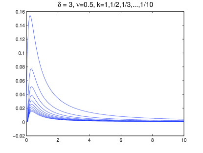
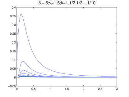
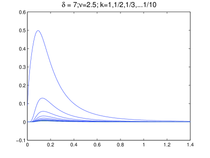
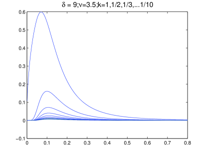
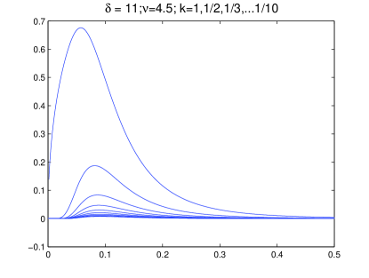
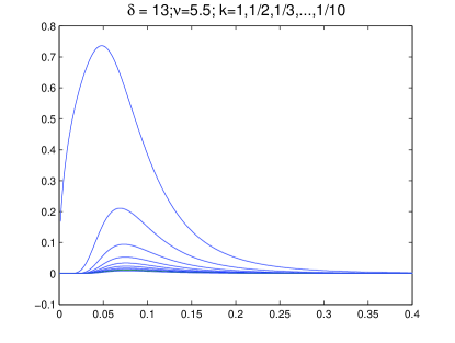
Figure 1. Varying $k$

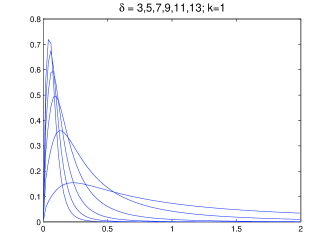
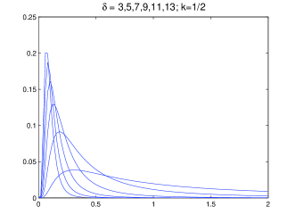
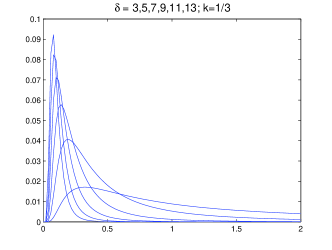
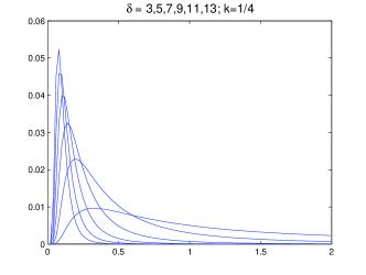
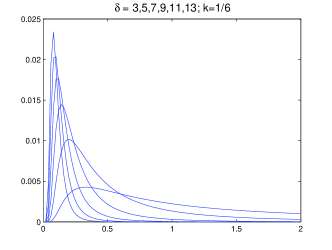
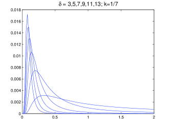
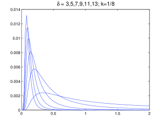
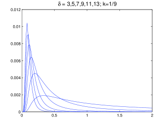
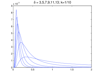
Figure 2. Varying $\delta$

References

- [1] Bentata, A. & Yor, M. Ten notes on three lectures: from Black-Scholes and Dupire formulae to last passage times of local martingales. Part A. The infinite time horizon, Preprint LPMA, No. 1223 (2008).
- [2] Bentata, A. & Yor, M. Ten notes on three lectures: from Black-Scholes and Dupire formulae to last passage times of local martingales. Part B. The finite time horizon, Preprint LPMA, No. 1232 (2008).
- [3] Getoor, R. K. The Brownian escape process. Annals of Prob., Vol. 7, No. 5, (October 1979), pp.864-867.
- [4] Kent, J. Some probabilistic properties of Bessel functions. Annals of Prob., Vol. 6, No. 5, (October 1978), pp.760-770.
- [5] Lebedev, N. N. Special functions & their applications. Translated by Silverman, R. R. Prentice-Hall, Inc. Englewood Cliffs, New Jersey, 1965.
- [6] Madan, D., Roynette, R., & Yor, M. Option prices as probabilities, Finance Research Letters 5, 79-87 (2008), doi:10.1016/j.frl.2008.02.002
- [7] Madan, D., Roynette, R., & Yor, M. An alternative expression for the Black-Scholes formula in terms of Brownian first and last passage times. Preprint IEC Nancy, No. 8 (2008).
- [8] Madan, D., Roynette, R., & Yor, M. From Black-Scholes formula to local times and last passage times for certain submartingales. Preprint IEC Nancy, No. 14 (2008)
- [9] Pal, S. & Protter, P. Strict local martingales, bubbles, and no early exercise. Preprint. arXiv:0711.1136, November 2007.
- [10] Pitman, J. & Yor, M. Bessel processes and infinitely divisible laws. Stochastic Integrals, ed.: Williams, D. Lecture Notes in Math 851, Springer (1981).
- [11] Revuz, D. & Yor, M. Continuous Martingales and Brownian Motion, Springer (1999), 3rd edition.
- [12] Salminen, P. On local times of a diffusion. Séminaire de Probabilité, XIX, eds. J. Azéma, M. Yor. LN in Mathematics, Vol. 1123 pp.63-79. Springer Verlag (1985).
- [13] Salminen, P. On last exit decompositions of linear diffusions. Studia Sci. Math. Hungarica, Vol. 33, p. 251-262 (1997).
- [14] Shiga, T. & Watanabe, S. Bessel diffusions as a one-parameter family of diffusion processes. Probability Theory and Related Fields, Vol 27, pp.37-46, Springer Berlin / Heidelberg (1973).