Numerical validation of the complex Swift-Hohenberg equation for lasers

Abstract

Order parameter equations, such as the complex Swift-Hohenberg (CSH) equation, offer a simplified and universal description that hold close to an instability threshold. The universality of the description refers to the fact that the same kind of instability produces the same order parameter equation. In the case of lasers, the instability usually corresponds to the emitting threshold, and the CSH equation can be obtained from the Maxwell-Bloch (MB) equations for a class C laser with small detuning. In this paper we numerically check the validity of the CSH equation as an approximation of the MB equations, taking into account that its terms are of different asymptotic order, and that, despite of having been systematically overlooked in the literature, this fact is essential in order to correctly capture the weakly nonlinear dynamics of the MB. The approximate distance to threshold range for which the CSH equation holds is also estimated.

I Introduction

The complex Swift-Hohenberg (CSH) equation is an order parameter equation that provides a reduced description of a variety of systems Cross and Hohenberg (1993), such as Rayleigh-Bénard convection Swift and Hohenberg (1977), optical parametric oscillators Longhi and Geraci (1996); Santagiustina et al. (2002); Hewitt and Kutzt (2005), Couette flow Manneville (2004), nematic liquid crystal Buka et al. (2004), magnetoconvection Cox et al. (2004), propagating flame front Golovin et al. (2003) and photorefractive oscillator Staliunas et al. (1995, 1997) among others. In the case of lasers operating near peak gain (small detuning), a derivation of the CSH equation for class A and C lasers was obtained in Lega et al. (1994, 1995), starting from the semiclassical Maxwell Bloch (MB) equations Risken and Nummedal (1968); Narducci et al. (1986); Lugiato et al. (1988); Coullet et al. (1989); Jakobsen et al. (1992), that provide a general description of transverse patterns in two levels, wide aperture and single longitudinal mode lasers. For class B lasers, such as CO₂ and semiconductor laser, CSH equations have been obtained in Barsella et al. (1999) and Mercier and Moloney (2002) respectively. (For an explanation of the classification of lasers, see Ref. Narducci and Abraham (1988).) Experimental observations of patterns in wide aperture lasers were reported in, for example, Dangoisse et al. (1992); Heckenberg et al. (1992); D’Angelo et al. (1992); Coates et al. (1994); Lippi et al. (1999). (For reviews on pattern formation in nonlinear optical systems, see Arecchi and Ramazza (1999); Lugiato et al. (1999); Staliunas and Sánchez-Morcillo (2003).)

The deduction of a generic order parameter equation greatly simplifies the theoretical description of the system. But it is important to note the limitation of this kind of model equations, as Cross and Hohenberg state in their review (Cross and Hohenberg, 1993, p. 874): “It is true that many properties of nonequilibrium systems are encountered in these equations, and indeed many hard problems (…) may profitably be addressed in the simple framework provided by these equations. However, it is only as a perturbative expansion valid in a small region near threshold that they provide a quantitative description of real experimental systems, and results may be even qualitatively misleading if applied far from threshold.”

We will focus our attention in a class C laser near peak gain that is assumed to be well described by the corresponding Maxwell Bloch equations. Using the assumptions that the amplitudes of the physical fields are small and depend slowly on time and on the transversal spatial scales, a CSH equation is derived form the Maxwell Bloch equations. The resulting CSH equation is that derived by Lega et. al. in Lega et al. (1994, 1995). Although not explicitly stated in this original formulation, the equation includes terms of different asymptotic order, in contrast to the Ginzburg Landau equation that is obtained for negative detuning Newell and Moloney (1992). This asymptotic nonuniformity is systematically obviated in the literature and was only recently addressed Martel and Hoyuelos (2006). It is the manifestation of the fact that dispersion and diffusion have necessarily different asymptotic order, and it affects the slow scales that the system develops near threshold.

The argument of a qualitative only scope of the model equation is usually invoked to justify the application of the CSH equation far from threshold. The qualitative correctness is difficult to be theoretically established, but, on the other hand, the capacity to produce quantitative predictions can be determined from the numerical integration of both, the original system of Maxwell Bloch equations and the CSH equation. The results of the comparison between the numerical simulations of the CSH and the MB equations is what we present in the subsequent sections of this paper. We can obtain from the simulations the relative error that introduces the approximation and estimate how far from threshold we can increase the pump while keeping a small relative error. Also, this numerical comparison between the CSH and the MB equations provides a confirmation of the main result presented in Martel and Hoyuelos (2006): that the CSH equation for the description of the weakly nonlinear dynamics of the system near threshold (derived in Lega et al. (1994, 1995)) necessarily contains terms of different asymptotic order.

II The complex Swift-Hohenberg equation and its numerical phase diagram

The Maxwell-Bloch equations for a two-level single longitudinal mode laser with flat mirrors are

$$\frac{\partial E}{\partial t}=ia\nabla^{2}E-\sigma E+\sigma P,$$ (1)

$$\frac{\partial P}{\partial t}=-(1+i\Omega)P+(r-N)E,$$ (2)

$$\frac{\partial N}{\partial t}=-bN+\frac{1}{2}(\overline{E}P+E\overline{P}),$$ (3)

where $E(x,y,t)$ and $P(x,y,t)$ represent the complex electric and polarization fields, and $N(x,y,t)$ is the real valued field of the population inversion (the same nondimensional formulation as in Ref. Newell and Moloney (1992) is used). Parameter $a>0$ is the strength of the diffraction (that we set to 1 by scaling the space variables), $\sigma>0$ is the cavity losses, $\Omega$ is the cavity detuning (the difference between atomic and resonance frequencies), $r$ is the pumping parameter, $b>0$ is the decay rate of the population inversion, $\nabla^{2}=\partial^{2}/\partial x^{2}+\partial^{2}/\partial y^{2}$ is the laplacian operator in the plane transverse to light propagation, and the bar stands for the complex conjugate. We will consider, as a specific case, a class C laser, for which $\sigma\sim 1$ and $b\sim 1$.

The corresponding CSH equation was obtained in Lega et al. (1994, 1995), and a simpler derivation method, in which no a priori relative scaling of the variables is assumed, was introduced in Martel and Hoyuelos (2006). A linear stability analysis of the Maxwell Bloch equations shows that the lasing instability takes place at a critical value of the pump $r_{c}=1$. The assumptions of small detuning and small distance to threshold,

$$|\Omega|\ll 1,|r-1|\ll 1,$$

are expressed through a small parameter $0<\varepsilon\ll 1$:

$$\Omega = \frac{(\sigma+1)^{2}}{\sigma}\omega\varepsilon,$$

$$r-1 = \frac{(\sigma+1)^{2}}{\sigma^{2}}(\omega^{2}+\alpha)\varepsilon^{2},$$ (4)

were $\alpha$ and $\omega$ are order 1 parameters that represent the scaled pump and detuning respectively.

The resulting CSH equation is of the from:

$$\phi_{\tilde{t}}=\alpha\phi+\textrm{i}\nabla^{2}\phi-\phi|\phi|^{2}-2\varepsilon\omega\nabla^{2}\phi-\varepsilon^{2}\nabla^{4}\phi,$$ (5)

where time and space were scaled as $\tilde{t}=\frac{(\sigma+1)}{\sigma}t\varepsilon^{2}$ and $(\tilde{x},\tilde{y})=\frac{(\sigma+1)}{\sqrt{\sigma}}(x,y)\varepsilon$.

This CSH equation is exactly the same as that obtained by Lega et. al. in Lega et al. (1994, 1995), but with the variables rescaled to show that it has terms of different asymptotic order and that it is not possible to remove the small parameter $\varepsilon$ from the equation. This asymptotic nonuniformity comes from the simple fact that dispersion involves second order spatial derivatives while double diffusion has fourth order ones and thus, in the long wave approximation where higher derivatives correspond to smaller terms, these two terms have necessarily different asymptotic order. This crucial fact is precisely what forced Lega et. al. Lega et al. (1994, 1995) to derive the CSH expanding first up to two orders (the first one included dispersion and the next the double-diffusion) and then collapsing back the expansion to get the CSH equation. But, despite of the wide use of the CSH equation, the asymptotic nonuniformity is never mentioned in the literature, and it was only recently analyzed in Martel and Hoyuelos (2006) where it was shown that it gives rise to two characteristic slow scales: one associated with dispersion $\delta_{\mathrm{disp}}$ and a second one associated with diffusion $\delta_{\mathrm{diff}}$. Using the scaling indicated above, $\delta_{\mathrm{disp}}\sim 1$ and $\delta_{\mathrm{diff}}\sim\sqrt{\varepsilon}\ll 1$, but in the original scaling of the Maxwell Bloch equation $\delta_{\mathrm{disp}}\sim 1/\varepsilon\gg 1$ and $\delta_{\mathrm{diff}}\sim 1/\sqrt{\varepsilon}\gg 1$, so both are long spatial scales.

The CSH equation above has to be considered in the close-to-threshold limit of $\varepsilon\rightarrow 0$, and the relation between the Maxwell Bloch and CSH solutions can be written as

$$\left[\begin{array}[]{c}E(x,y,t)\\ P(x,y,t)\\ N(x,y,t)\end{array}\right]=\left[\begin{array}[]{c}1\\ 1\\ 0\end{array}\right]\sqrt{b}\frac{(\sigma+1)}{\sigma}\textrm{e}^{-i\sigma\omega\tilde{t}/\varepsilon}\phi(\tilde{x},\tilde{y},\tilde{t})\,\varepsilon+O(\varepsilon^{2}),$$ (6)

Traveling wave solutions of the form $\phi_{\rm{TW}}=\sqrt{\alpha}\>\textrm{e}^{\textrm{i}\mathbf{k}_{\rm{TW}}\cdot\tilde{\mathbf{x}}-\textrm{i}k_{\rm{TW}}^{2}\tilde{t}}$, with $k_{\rm{TW}}=|\mathbf{k}_{\rm{TW}}|\sim 1$ are approximate solutions of the CSH equation up to $O(\varepsilon)$ corrections (this family of TW is just the result of making the limit $\varepsilon\rightarrow 0$ and $k\sim 1$ in the well known expression of the exact TW family, see Oppo et al. (1991); Jakobsen et al. (1992, 1994); Lega et al. (1994, 1995)). This solution exists only for $\alpha>0$ and a linear stability analysis shows that it becomes unstable outside the region defined by $\omega>0$ and $\alpha>\omega^{2}$ with a critical wavenumber $k_{c}=\sqrt{\omega/\varepsilon}\gg 1$ Martel and Hoyuelos (2006), which corresponds to a perturbation with small diffusive length scale. The phase diagram in the parameter space $\alpha$-$\omega$ represented in Fig. 1 was numerically reproduced starting with an initial condition with $\mathbf{k}_{\rm{TW}}=(1,1)\,2\pi/3$ plus noise of amplitude 0.02. The system has been integrated using periodic boundary conditions in a square box of length 3. The mesh of Fig. 1 represents the final states for the corresponding values of $\alpha$ and $\omega$, for $\tilde{t}=10$ and $\varepsilon=0.0083$ (each square in the mesh is the result of an individual numerical integration). To the right of the parabola $\alpha=\omega^{2}$ the traveling wave solution becomes unstable and gives rise to another structure with smaller wavelength associated with the diffusive terms in Eq. (5). Some squares of the mesh still show the long wavelength solution to the right of the parabola, where it should be unstable. The reason is that, close to the stability limit, the unstable modes require a time greater than $\tilde{t}=10$ to grow.

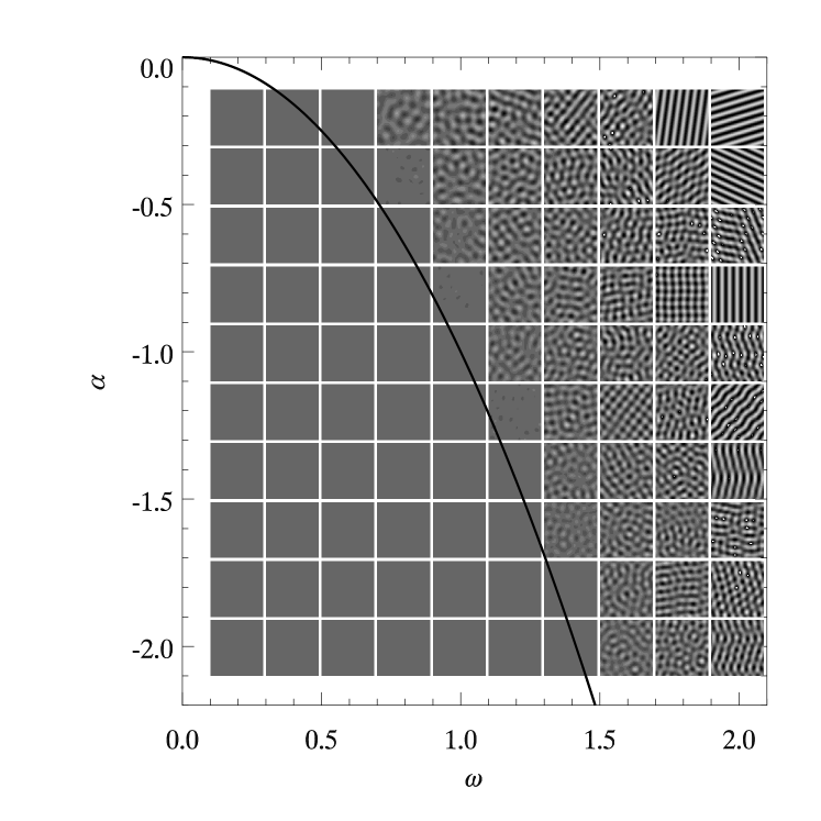
Figure 2: Real part of $\phi$ for different points in the region of parameter space $\alpha<0$ and $\omega>0$. Each square represents an individual numerical integration of Eq. (5) with initial condition given by the nonlasing solution, $\phi=0$, plus Gaussian noise of amplitude 0.2. The curve $\alpha=-\omega^{2}$ is the stability limit of the zero solution. The final time is $\tilde{t}=10$ and $\varepsilon=0.0083$. The gray scale values are: black $=-2.5$, gray $=0$, and white $=2.5$

The nonlasing solution, $\phi=0$, is linearly unstable for $\alpha>0$ if $\omega<0$, and for $\alpha>-\omega^{2}$ if $\omega>0$ (exhibiting again a large diffusive critical wavenumber $k_{c}=\sqrt{\omega/\varepsilon}\gg 1$) Martel and Hoyuelos (2006). The numerical phase diagram of Fig. 2 confirms again the theoretical stability predictions and shows the appearance of a structure with wavenumber $k\sim 1/\sqrt{\varepsilon}\gg 1$ to the right of the stability limit given by the parabola $\alpha>-\omega^{2}$. The initial condition is Gaussian noise with amplitude 0.2, the final time is $\tilde{t}=10$ and $\varepsilon=0.0083$.

In the next section we will analyze the dynamics in two representative points of the phase diagram: $\alpha=0.75$, $\omega=0.5$ (pattern with dispersive scale $\delta_{\mathrm{disp}}\sim 1$), and $\alpha=0.5$, $\omega=2$ (pattern with diffusive scale $\delta_{\mathrm{diff}}\sim\sqrt{\varepsilon}$).

III Numerical validation

We numerically check the accuracy of the CSH equation (5) as a reduced dynamics of the Maxwell Bloch equations (1)-(3). The difference between both descriptions is computed as

$$d=\left|\left|\left[\begin{array}[]{c}E(x,y,t)\\ P(x,y,t)\\ N(x,y,t)\end{array}\right]-\left[\begin{array}[]{c}1\\ 1\\ 0\end{array}\right]\sqrt{b}\frac{(\sigma+1)}{\sigma}\textrm{e}^{-i\sigma\omega\tilde{t}/\varepsilon}\phi(\tilde{x},\tilde{y},\tilde{t})\,\varepsilon\right|\right|.$$ (7)

Symbols $||\cdot||$ denote the Euclidian norm on $\mathbb{C}^{3N}$ divided by $\sqrt{N}$, where $N$ is the number of points of the discretized system. So, $d$ is an average absolute error, that, according to the weakly nonlinear procedure applied to the MB equations to derive the CSH equation, has to behave as $d\sim\varepsilon^{2}$; see Eq. (6).

There is a severe numerical difficulty in integrating Eq. (5) due to the presence of two spatial scales, $\delta_{\mathrm{disp}}\sim 1$ and $\delta_{\mathrm{diff}}\sim\sqrt{\varepsilon}$, which are very different in the relevant limit $\varepsilon\rightarrow 0$ and should be simultaneously well resolved. We consider a one dimensional system, with periodic boundary conditions, in order to reduce the size of the computations and be able to use a greater system length than would be possible in higher dimensions. We let the system evolve until the difference $d$ reaches a stationary value $d_{s}$. For the parameters used, a time $\tilde{t}\sim 10$ is enough to reach a stationary state, and the corresponding maximum integration time for the MB equations is $t\sim 10/\varepsilon^{2}$. Therefore, to check the asymptotic theoretical behaviour for $\varepsilon\rightarrow 0$, we need a large number of Fourier modes and long time. The CSH and MB equations are integrated in Fourier space using a fourth-order Runge-Kutta scheme, with 1024 Fourier modes, $\sigma=b=1$, time step $dt=0.01$ ($d\tilde{t}=2\,dt\,\varepsilon^{2}$), space step $d\tilde{x}=1/1024$ [$dx=d\tilde{x}/(2\varepsilon)$], and $\varepsilon$ in the range between 0.0011 and 0.025.

The initial condition for $\phi$ is filtered Gaussian noise of amplitude 1. Since Eq. (5) does not include spatial scales smaller than $\delta_{\mathrm{diff}}\sim\sqrt{\varepsilon}$, the modes with wavenumber greater than $k\sim 1/\sqrt{\varepsilon}$ are initially filtered. The initial condition for $(E,P,N)$ is obtained from the one for $\phi$ using Eq. (6). In Fig. 3 we show the real and imaginary part of $\phi$ at $\tilde{t}=0$ and $\tilde{t}=5$, for $\varepsilon=0.0011$, $\alpha=0.5$ and $\omega=2$.

In order to calculate an average relative error, we divide $d$ by $\varepsilon$, the typical magnitude of the fields in the Maxwell Bloch equations (note that $\phi$ is of order 1). In Fig. 4 we plot $d/\varepsilon$ in log scale against $\tilde{t}$, for different values of $\varepsilon$ and for $\alpha=0.5$ and $\omega=2$.

We consider the stationary value of the relative error for long times $(d/\varepsilon)_{s}$, and check the theoretical asymptotic behaviour $(d/\varepsilon)_{s}\sim\varepsilon$. In Fig. 5 we plot $(d/\varepsilon)_{s}$ against $\varepsilon$ for two points in parameter space: $\alpha=0.75$, $\omega=0.5$; and $\alpha=0.5$, $\omega=2$. In both cases, the linear behaviour $(d/\varepsilon)_{s}\sim\varepsilon$ is confirmed. But the numerical result offers a new important figure: the slope. The slopes are $3.6\pm 0.1$ for $\alpha=0.75$, $\omega=0.5$; and $18\pm 1$ for $\alpha=0.5$, $\omega=2$. The increase of the slope in the second case is related to the fact that patterns with smaller length scales appear for $\alpha=0.5$, $\omega=2$ (see Fig. 1).

An experimental confirmation of the CSH equation would require to know a specific value of the appropriate distance to threshold for which the equation is valid. Let us suppose that the sought experimental confirmation has a maximum relative error of 10% and make the favorable assumptions that the Maxwell Bloch equations accurately describe the experiment and that the chosen parameters correspond to a simple pattern with characteristic length equal to $\delta_{\mathrm{disp}}\sim 1$ as, for example, for $\alpha=0.75$, $\omega=0.5$. Then, using the slopes of Fig. 5, we can calculate that the distance to threshold should not exceed $r-1=0.003$, and the pump must be tuned with a relative error smaller than 0.3%. For $\alpha=0.5$, $\omega=2$, where patterns with diffusive scale $\delta_{\mathrm{diff}}\sim\sqrt{\varepsilon}$ arise, the situation is worse since the maximum distance to threshold is $r-1=0.0006$, and the relative error of the pump should be smaller than 0.06%.

IV Conclusions

We performed numerical integrations of the Maxwell Bloch equations and the corresponding CSH equation, for a class C laser. The CSH equation gives a simplified and reduced dynamics of the original Maxwell Bloch equations for small detuning. Comparing the results produced by both set of equations, we obtain an average relative error of the CSH equation solutions. The numerical results confirm the following theoretical prediction: $(d/\varepsilon)_{s}\sim\varepsilon$, where $(d/\varepsilon)_{s}$ is the stationary relative error that is reached for long times (the small parameter $\varepsilon$ is introduced in the deduction of the CSH equation and is directly related to the detuning and distance to threshold). Therefore, as expected, the CSH equation with terms of different asymptotic order Martel and Hoyuelos (2006) is the appropriate envelope equation to accurately represent the behaviour of the Maxwell Bloch equations when $\varepsilon\rightarrow 0$.

The numerical results also allow us to estimate the distance to threshold range for which the CSH equation holds. Assuming an average relative error of 10%, the maximum distance to threshold is between 0.003 and 0.0006 for the parameter values analyzed: $\alpha=0.75$, $\omega=0.5$, and $\alpha=0.5$, $\omega=2$. The most restrictive value (0.0006) corresponds to the case when the resulting pattern has diffusive scales ($\delta_{\mathrm{diff}}\sim\sqrt{\varepsilon}$). Although it is not unfeasable to experimentally establish such small distance to threshold, it requires a fine tuning of the pump that is not usually available in standard lasers. Another important experimental difficulty is to obtain a wide enough beam for the patterns to develop.

Finally, it is important to mention that, despite of the problems for setting up an accurate laser experiment in the CSH range, the numerical results on this paper confirming the validity of the CSH equation are interesting and valuable from the more general point of view of Pattern Formation. The CSH equation is an envelope equation and it is universal in the sense that its structure depends only on the kind of instability of the problem and not on the particular physical problem under consideration.

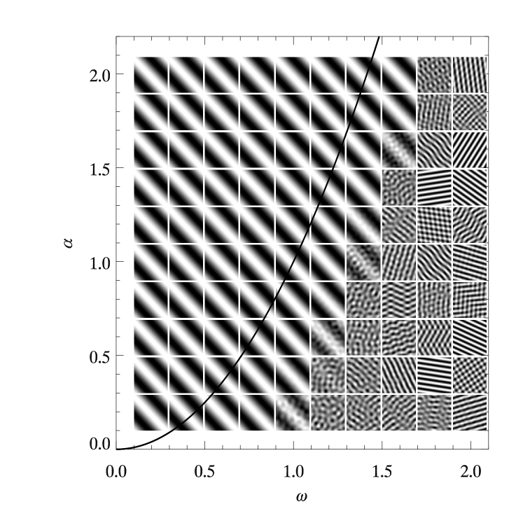
Figure 1: Real part of $\phi$, in a 2D system of size 3$\times$3 with periodic boundary conditions, for different points in the region of parameter space $\alpha>0$ and $\omega>0$. Each square represents an individual numerical integration of Eq. (5) with initial condition given by a traveling wave, with $\mathbf{k}_{\rm{TW}}=(1,1)\,2\pi/3$, plus noise of amplitude 0.02. The curve $\alpha=\omega^{2}$ is the stability limit of this kind of solution. The final time is $\tilde{t}=10$ and $\varepsilon=0.0083$. The gray scale limit values are: black $\simeq-2.5$ and white $\simeq 2.5$

Figure 3: Real (continuous line) and imaginary (dashed line) parts of $\phi$ in a 1D system of size 1 and periodic boundary conditions. Top: the initial condition given by filtered Gaussian noise. Bottom: final state for $\tilde{t}=5$. Parameters are $\varepsilon=0.0011$, $\alpha=0.5$ and $\omega=2$.

Figure 4: Average relative error $d/\varepsilon$ in log scale against time $\tilde{t}$ for different values of $\varepsilon$. From top to bottom, $\varepsilon=0.025,0.018,0.013,0.0088,0.0063,0.0044,0.0031,0.0022,0.0016$ and $0.0011$. Parameters are $\alpha=0.5$ and $\omega=2$

Figure 5: Stationary relative error $(d/\varepsilon)_{s}$ against $\varepsilon$. Plus symbols correspond to $\alpha=0.75$, $\omega=0.5$ (slope $3.6\pm 0.1$); and asterisks to $\alpha=0.5$, $\omega=2$ (slope $18\pm 1$).