The Chiral Magnetic Effect
Abstract
Topological charge changing transitions can induce chirality in the quark-gluon plasma by the axial anomaly. We study the equilibrium response of the quark-gluon plasma in such a situation to an external magnetic field. To mimic the effect of the topological charge changing transitions we will introduce a chiral chemical potential. We will show that an electromagnetic current is generated along the magnetic field. This is the Chiral Magnetic Effect. We compute the magnitude of this current as a function of magnetic field, chirality, temperature, and baryon chemical potential.
I Introduction
The quark-gluon plasma is a phase of extremely hot matter consisting of quarks and gluons. Just after the Big-Bang, the universe itself was in the quark-gluon plasma phase. The quark-gluon plasma can be created and studied using collisions of heavy ions. An active experimental program to investigate the properties of this hot phase of matter is underway using the Relativistic Heavy Ion Collider (RHIC) at BNL. In the near future the quark-gluon plasma will also be studied using the Large Hadron Collider (LHC) at CERN, the Facility for Antiproton and Ion Research (FAIR) at GSI, and the NICA facility at JINR, Dubna.
The behavior of the quark-gluon plasma is described by Quantum Chromodynamics (QCD). One of the intriguing predictions of QCD is that in the quark-gluon plasma phase certain special gluon configurations to which one can assign a winding number play a role BPST ; H . This winding number is a topological invariant, which means that smooth deformations of these configurations do not change the winding number. Experimental evidence for the existence of configurations with nonzero winding number is only indirect from the meson spectrum Witten:1979vv ; 'tHooft:1986nc ; Chu:1994vi .
The configurations with nonzero winding number are in fact transitions which invoke passing a potential barrier with a height of order the QCD scale over the strong coupling constant . Because of the height of the barrier, the transitions are highly suppressed at low temperatures since they require tunneling H . The configurations responsible for this tunneling process are called instantons H ; 'tHooft:1986nc ; GPY ; SS98 . At high temperatures in the quark-gluon plasma phase, it is possible to jump over the potential barrier. The transitions are therefore not suppressed anymore and called sphalerons M83 ; KM84 ; KRS ; AM87 ; KS88 ; AM88 . These configurations were studied in the electroweak theory as a mechanism for baryogenesis KRS ; AM87 ; AM88 ; Shaposhnikov1987 , and are also relevant for QCD MMS ; GZ94 ; SZ03 .
At these high temperatures the configurations with nonzero winding number can be produced with relatively high probability MMS ; BMR . Therefore the quark-gluon plasma is the best place to find direct experimental evidence for the existence of gauge field configurations with nonzero winding number.
These configurations do something very distinct to quarks; they can, depending on the sign of their winding number, transform left- into right-handed quarks or vice-versa via the axial anomaly ABJ (see also C80 ; S92 ). For massless quarks, the axial anomaly equates to the topological term. The spatial integration of yields an exact relation for the rate of the chirality change induced by topological configurations, which reads
| (1) |
where denotes the net number of quarks (minus antiquarks) with right/left-handed chirality, the number of massless flavors, and , with . All the massless flavors equally couple to the gauge field, hence the proportionality factor arises in Eq. (1). Let us stress that, in the common convention, chiral quarks have opposite helicity to antiquarks; a particle with right-handed chirality has right-handed helicity, while an anti-particle with right-handed chirality has left-handed helicity. For instance the helicity of the antineutrino is right-handed. Here right-handed helicity means spin and momentum parallel, while left-handed helicity means spin and momentum anti-parallel. Therefore the difference can also be read as the total number of quarks plus antiquarks with right-handed helicity minus the total number of quarks plus antiquarks with left-handed helicity. For physical gluon configurations (configurations with finite action) the time integral over the right-hand side of Eq. (1) is equal to minus twice the winding number of the gluon field configuration. As a result of the axial anomaly the interactions between these configurations and the quarks break the parity () and charge-parity () symmetry. Ordinary (perturbative) interactions between quarks and gluons cannot induce a difference between the number of right- and left-handed quarks. A mass term always will tend to wash out such difference AGP .
In QCD, the probability to generate either a gluon configuration with positive or negative winding number is equal. This is because there is no direct and violation in QCD (assuming the value of the angle is equal to zero). In the quark-gluon plasma, many of these configurations can be generated at different points in space and time with different winding numbers. In pure Yang-Mills theory this process is completely random; the dynamics of the chirality change is that of a one-dimensional random walk. In QCD with massless flavors, however, it will cost energy to induce a difference between the number of right- and left-handed quarks because of the Fermi-principle. Therefore the dynamics is not completely random anymore, and there is a preference to decrease the chirality MMS . In any case, the variance of the chirality will be nonzero, and increase as a function of time according to diffusion. Hence, it is expected that every time the quark-gluon plasma is produced, it will posses a non-zero chirality KKV . The chirality averaged over many events of quark-gluon plasma production vanishes. Therefore one speaks in this case of event-by-event - and -violation.
Next to the sphaleron transitions, chirality could also be introduced in the quark-gluon plasma in the same way due to chromoelectric and chromomagnetic fields in the initial state of the quark-gluon plasma produced in heavy-ion collisons, i.e. the so-called glasma KKV ; LM06 ; KKL . Although the net topological charge cannot develop with the Boost invariant configuration KKV , the glasma instability spontaneously breaks the Boost invariance glasmainst , so that the event-by-event topological charge fluctuation is expected. The situation is then quite reminiscent of the sphaleron transitions LM06 .
It was first argued by one of us K06 that if - and -violating processes are taking place in the quark-gluon plasma produced in heavy-ion collisions, then positive charges should separate from negative charges along the direction of angular momentum of the collision. In Ref. KZ this mechanism was worked out in more detail using an effective angle to mimic - and -violating processes. In heavy-ion collisions the magnetic field is pointing in the direction of angular momentum. It was shown in Ref. KZ that this magnetic field induces charge on a -domain-wall in such a way that an electric field is created parallel to the magnetic field. In this way positive charge is separated from negative charge along the magnetic field. In Ref. KMW a different mechanism for charge-separation was discussed (see also WQM ). It was shown that a magnetic field in the presence of imbalanced chirality induces a current along the magnetic field. Again, as a result, positive charge is separated from negative charge along the magnetic field. This is called the “Chiral Magnetic Effect”.
Due to the separation of charge along the direction of the magnetic field in heavy-ion collisions, an asymmetry between the amount of positive/negative charge above and below the reaction plane is expected K06 ; KZ ; KMW . These asymmetries can be analyzed in experiments using a correlation study as proposed by Voloshin V04 . Preliminary data from the STAR collaboration is presented in Refs. IVS ; VQM . Observation of the Chiral Magnetic Effect will be direct experimental evidence for the existence of topologically non-trivial gluon configurations. It furthermore is evidence for event-by-event - and -violation.
The Chiral Magnetic Effect could be used to determine whether a deconfined chirally symmetric phase of matter is created in heavy-ion collisions KMW . Deconfinement is a necessary requirement for the Chiral Magnetic Effect to work, since it requires that soft quarks can separate over distances much greater than the radius of the nucleon. Moreover, chiral symmetry restoration is essential, because a chiral condensate will tend to erase any asymmetry between the number of right- and left-handed fermions.
In this article we will investigate the Chiral Magnetic Effect in detail. In order to treat the non-vanishing chirality, we introduce a chiral chemical potential, denoted as . The chiral chemical potential will be generated by the topological charge changing transitions. We will not study this dynamical process, but we just assume this chemical potential is there. Then we will study the implications of applying a magnetic field to a system with nonzero chiral chemical potential in equilibrium. We will see that an electromagnetic current will be induced in the direction of the magnetic field. We will compute the magnitude of this current as a function of magnetic field, chirality, temperature, and baryon chemical potential.
Besides the Chiral Magnetic Effect, the fact that a magnetic field can influence QCD processes is well known. For example a magnetic field can induce chiral symmetry breaking GMS , influence the chiral condensate SS97 ; CMW , and therefore modify the phase diagram of QCD (see Refs. FM ; AF for recent discussions). Also the color-superconducting phases predicted to exist at high baryon densities are strongly affected by a strong magnetic field ABR ; FIM ; FW ; NS . Finally the anomaly in the presence of a magnetic field can give rise to all kinds of interesting effects, like spontaneous creation of axial currents SZ04 ; MZ and formation of -domain walls SS08 .
The analysis we present in this article can be used to make predictions for the charge asymmetries in heavy-ion collisions like are done in Ref. KMW . We will encounter the beautiful physics of the anomaly, current quantization and the index theorem, and periodic oscillatory behavior due to Landau level quantization.
II Chiral chemical potential
As was argued in the introduction, topological charge changing transitions can induce an asymmetry between the number of right- and left-handed quarks due to the axial anomaly. In order to study the effect of this asymmetry we introduce a chiral chemical potential . This chemical potential couples to the difference between the number of right- and left-handed fermions. To the Lagrangian density the following term is added
| (2) |
The energy spectrum of the free Dirac equation in the presence of a chiral chemical potential is for massless modes (with for simplicity),
| (3) | |||
| (4) |
Here represents the spin in the -direction and , the chirality. The momentum in the -direction is given by ; let us stress that in our notation does not denote the third component of a four-vector with metric convention. We have displayed the massless energy spectrum in Fig. 1. In the massless limit one can distinguish modes with right-handed chirality from modes with left-handed chirality. It should be mentioned that is restricted to be positive for the and particle modes so that the helicity is positive for and negative for , respectively, and is negative for the and particle modes (see Fig. 1). If the chiral chemical potential is positive some of the right-handed particle modes will become occupied while some of the left-handed anti-particle modes will be filled as well. A net chirality is created in this way.

The chiral chemical potential lifts the degeneracy between modes with right- and left-handed chirality. A difference between the total number of particles plus anti-particles with right-handed and left-handed helicity is created. The magnetic field will lift the degeneracy in spin depending on the charge of the particle. Hence particles with right-handed helicity will tend to move opposite to anti-particles with right-handed helicity. As a result an electromagnetic current is generated along the magnetic field, which is the Chiral Magnetic Effect KMW (see also Refs. KMW ; WQM for a pictorial representation of the Chiral Magnetic Effect). We will compute this induced electromagnetic current in the next section.
The effect of a finite amount of topological charge change can also be mimicked by an effective theta angle, which could depend on space-time (see for example K06 ; KZ ; KPT ). One adds to the Lagrangian of QCD the following term,
| (5) |
By performing an axial U(1) rotation this term can be transformed into the following fermionic contribution
| (6) |
Identifying this with Eq. (2) we see that . We can also identify with the time component of an axial vector field . The effective theta angle results in a difference between the rates of changing left-handed into right-handed and changing right-handed into left-handed particles. The chiral chemical potential, however, is a more static quantity; it is the energy necessary to put a right-handed quark on its Fermi surface or to remove a left-handed quark from its Fermi surface. It describes the difference between the number of right- and left-handed fermions. An effective theta angle to describe spontaneous and -violating processes has been discussed often in the literature (for examples see Refs. K06 ; KZ ; KPT ; theta ). The chiral chemical potential has on the other hand only been used in a few papers NM ; MMS ; SSS98 ; JPT .
Let us finally point out that the chiral chemical potential has no sign problem, i.e. the fermionic determinant with is real and positive. In the presence of a chiral chemical potential the fermionic determinant reads in Euclidean space-time,
| (7) |
where . Here we have chosen a representation in which all matrices are Hermitian, . Since and are anti-Hermitian the eigenvalues of are of the form , where . Because anticommutes with , all eigenvalues come in pairs, which means that if is an eigenvalue, also is an eigenvalue. Since the determinant is the product of all eigenvalues we see that the determinant is the product over all of . Hence the determinant is real and also positive semi-definite. This is very interesting because it allows for a lattice QCD simulation of chirally asymmetric systems. The lattice QCD can then simulate the Chiral Magnetic Effect by introducing a space-dependent phase on the link variable which amounts to the external magnetic field.
III Computation of Induced Current
In this section we will show if a magnetic field is applied to a system with an asymmetry between the number of right- and left-handed fermions, an electric current is induced along the magnetic field. We will compute this current in four different ways, since we think they are all very instructive. The first way is through an energy balance argument. Then we will arrive at the result by solving the Dirac equation. The third way is by explicitly computing the thermodynamic potential in the presence of a magnetic field. The last derivation we discuss is using a derivative expansion of the effective action. We will compute the current for a generic fermion with electric charge and neither flavor nor color; at the end of this section we will discuss what happens if we recover the flavor and color for quarks.
Let us set up notation. We will take the metric and the chiral representation for the gamma matrices;
| (8) |
where and are the quaternion bases. Using this convention it is possible to write the fermion field into its left- and right-handed components . We define the right- and left-handed chemical potentials as and . Here denotes the quark chemical potential, which for three colors () is equal to one third of the baryon chemical potential. If we write , as we mentioned in the previous section, we mean the -component of the momentum vector and not the third component of the four-vector .
The total current is equal to the volume integral over the current density,
| (9) |
The current density is given by the following expectation value,
| (10) |
Here the expectation value is over a thermodynamic ensemble. One can write the current density in terms of right- and left-handed spinors as
| (11) |
III.1 Axial anomaly and the energy balance
The easiest way to obtain the right expression for the current is using a beautiful argument of energy balance by Nielsen and Ninomiya NM . Consider a situation with an electric field and a magnetic field in the presence of a chiral chemical potential. In that case the electromagnetic anomaly will tell us that the rate of change of chirality is equal to the volume integral over . There exists an intuitive derivation of this rate NM which we will repeat here.
Let us consider fermions with positive charge in a background magnetic field . The fermions will occupy Landau levels, so their motion in the transverse (to the field ) plane will be restricted. The fermions however are free to move along or opposite the direction of ; since the spins of the fermions are preferentially aligned along the field, the motion parallel to corresponds to the right-handed fermions, and anti-parallel to – to left-handed fermions.
The presence of an electric field parallel to causes the chirality to change (see Ref. Witten:1984eb for a related discussion of particle acceleration in cosmic strings). The energy of right-handed fermions moving along the electric field under the influence of the Lorentz force will grow linearly with time, leading to the growing Fermi momentum,
| (12) |
Likewise, for left-handed charges the Fermi momentum will decrease, with ; this corresponds to the production of left-handed anti-particles with charge . Therefore the particles with charge will move along the field, and anti-particles with charge , against the field. Thus, an electric current is created along .
The density of right-handed fermion states is equal to the product of the longitudinal phase space density and the density of Landau levels in the transverse direction ,
| (13) |
The same expression yields also the density of left-handed anti-fermion states; therefore, the rate of chirality generation per unit volume per unit time is then given by
| (14) |
We have thus reproduced the general anomaly relation for the electromagnetic fields.
Consider now the energy balance related to the chirality change. To change a left-handed fermion in a right-handed fermion requires removing a particle from the left-handed Fermi surface and adding it to the right-handed Fermi-surface. This will cost an energy or . So multiplying this energy by the rate of chirality change we know how much energy is needed per unit of time. This energy has to come from somewhere, assuming no losses; it will be equal to the power delivered by a current. This power is equal to the product of the current with the electric field. So one finds NM
| (15) |
We can take in the direction of in this expression. Then if we take the limit we find
| (16) |
This derivation clearly shows that not only the axial anomaly of QCD plays a role in the Chiral Magnetic Effect, but also the electromagnetic axial anomaly. The QCD anomaly provides the chirality, the electromagnetic anomaly the current. In a box with periodic boundary conditions, the number of Landau levels is an integer. This gives rise to current quantization as we will closely see in the next microscopic derivation.
III.2 Dirac equation
We will now compute the induced current by solving the Dirac equation in the presence of a magnetic field and chiral chemical potential. We take the magnetic field in the -direction,
| (17) |
The Dirac equation in this background reads
| (18) |
where . In order to incorporate the magnetic field given in Eq. (17) the only non-vanishing components of are . Furthermore only will depend on and . The precise form of is not relevant for our calculation.
We will compute the total current in the -direction as is given in Eq. (9) starting from Eq. (11). To proceed one has to make a momentum decomposition of the fields in terms of creation and annihilation operators. As is shown explicitly in Ref. MZ the only non-vanishing contribution to
| (19) |
arises from the transverse zero modes, i.e. modes which have . The reason is that in all the non-zero modes there is a spin degeneracy in energy, which results in the cancellation of the expectation value of AC ; MZ . The transverse zero-modes are however not degenerate. Let us denote the number of transverse zero modes with equal to as . One shows that the difference is equal to the index of a two-dimensional Dirac Hamiltonian in the presence of a magnetic field AC . This index can be expressed in terms of the total flux . One finds AC ; MZ
| (20) |
where we have introduced the floor function which is the largest integer smaller than . The flux is equal to the integral of the magnetic field over the transverse plane,
| (21) |
Let us stress here that the number of zero modes is quantized, and not the magnetic flux itself.
It is now possible to construct the total current. It is equal to the sum of number densities in the transverse zero-mode weighted by the spin degeneracy . For the right-handed modes we find
| (22) |
Here denotes the length of the system in the -direction and is the Fermi-Dirac distribution. The two Fermi-Dirac distributions in Eq. (22) correspond to right-handed particle and antiparticle modes respectively. In front of the antiparticle contribution there is a minus sign, since is the number density of particles minus antiparticles. The temperature dependence has dropped out from Eq. (22) without approximation. The reason why runs only positive is, as we have explained on Fig. 1, has positive only and has negative whose sign we changed in the integral. Similarly, for the left-handed modes we find,
| (23) |
By taking the spin sum and subtracting L from R contributions we find that the total current becomes
| (24) |
The result is independent of temperature and density. By adding the two contributions one finds the total induced axial current, in the massless limit,
| (25) |
This current was computed for by Metlitski and Zhitnitsky MZ . We recover the result of Ref. MZ and find that the total axial current is independent of .
This derivation can be performed in the more general case with massive fermions. The computation is more involved, but the final answer will turn out to be independent of mass. In the next derivation we will include a mass term and show that the answer is independent of mass. There, it will be transparent why the result is insensitive to temperature and density as well. The last derivation using the derivative expansion will provide understanding why the current is independent of mass from a different point of view.
III.3 Thermodynamic potential
We will now derive the current in a homogeneous magnetic background using the thermodynamic potential. In the presence of a chiral chemical potential we find that the thermodynamic potential is given by
| (26) |
where is a sum over Landau levels, is a sum over spin and the dispersion relation is given by
| (27) |
The first term in the square brackets may also be written as without the sign function. The constant ensures that the lowest Landau level only contains one spin component,
| (28) |
We also note again that the phase space associated with Landau levels is quantized in a box with periodic boundary conditions. We omit this to avoid bothersome notation like in the phase space factor.
Let us introduce a constant gauge field . One might think that a constant gauge field could be gauged away, but this is not possible by a gauge transformation satisfying the periodic boundary condition. The current density is the derivative of the thermodynamic potential with respect to at the point ,
| (29) |
The thermodynamic potential is still given by Eq. (26), but the dispersion relation Eq. (27) is now modified by replacing by . In order to regularize the ultraviolet divergences of thermodynamic potential we introduce a momentum cutoff on the integral. Furthermore we introduce a cutoff on the sum over the Landau levels. After we have introduced this regularization we can pull the derivative with respect to through the sum and integral. Then we can use that
| (30) |
when acting on an arbitrary function of . As a result we find the following expression for the current density,
| (31) |
where is now given by Eq. (27) since we used that has to put to zero after taking the derivative. After summing over spins the contribution to the integrand of the Landau Levels with is an odd function of . Hence only the lowest Landau level which contains one spin component contributes to the current. As a result for we find
| (32) |
where
| (33) |
For one has to replace by in Eq. (32). Since the integrand is a total derivative, it is easily integrated. The medium part (logarithmic term) drops because it goes to zero with . Only a surface term remains, which equals
| (34) |
where we have used that corresponds to the sign of . The fact that the current is equal to a surface term is because it is caused by the electromagnetic anomaly. This as was argued in the first derivation.
By multiplying the current density Eq. (34) with the volume one finds the total current Eq. (24). The virtue in this derivation is that it is manifest that the current results from the surface integral at infinitely large momentum, to which any infrared effects of mass, temperature, and are irrelevant. The next derivation using the derivative expansion will give us more understanding why this result is independent of mass.
III.4 Derivative expansion of effective action
The last derivation of the current we discuss is by using a derivative expansion of the effective action as is performed by D’Hoker and Goldstone HG (see also BO ). Let us introduce an axial vector field and write the covariant derivative as . One can define right- and left-handed vector fields as follows: and . By performing the integration over the fermions fields one obtains the following effective action
| (35) |
Here includes the space-time coordinates as well as the color and Dirac indices. The current density can be obtained by taking the functional derivative of this expression with respect to . In the presence of an axial vector field the divergence of a vector current is anomalous; one has HG
| (36) |
One can write down an expansion of the current in terms of the fields , and their derivatives. The expression should be Lorentz covariant and gauge invariant. Furthermore the current should satisfy the anomaly constraint Eq. (36). To first order in the fields and derivatives one obtains HG ,
| (37) |
The current is -independent. This follows directly from the anomalous divergence of the vector current, that has no -dependent contributions even with inclusion of a mass term. However, the divergence of the axial vector current is -dependent. Therefore the axial vector current induced by a magnetic field depends on mass. This is indeed found in Ref. MZ .
We can now use that in Eq. (37), so that we obtain the current density induced by a magnetic field,
| (38) |
Since the last equation was obtained via a derivative expansion, the derivation assumes constant magnetic fields.
III.5 Discussion of derivations
We have argued in Sec. II that up to a coupling constant. Suppose we have a space-dependent theta angle , for example formed by a domain wall. The covariant current in Eq. (37) shows that an electric field will induce a current perpendicular to the electric field on the domain wall. Moreover, it shows that a magnetic field will induce charge on the domain wall. The generation of charge on domain walls or solitons was first discussed by Goldstone and Wilczek GW . Callan and Harvey CH have studied this mechanism as well in the context of axionic cosmic strings. They however use pseudoscalar coupling instead of axial vector coupling, but find a result for the current which is equivalent to Eq. (37). It was argued in Refs. BDF ; FDB that on domain walls formed in certain semi-conductors currents could be generated perpendicular to the electric field for the same reason. In the context of charge separation in heavy-ion collisions, the generation of charge on domain walls was discussed by Kharzeev and Zhitnitsky KZ .
Goldstone and Wilczek GW have derived their current using a perturbative one-loop calculation. It is also possible to compute our current perturbatively. One obtains a triangle one-loop diagram with two vector couplings and one axial vector coupling. As is well known, this diagram contains the anomaly. If one includes the effect of the chiral chemical potential in the fermion propagator, the diagram to compute is the photon polarization tensor.
The axial anomaly generates the topological term which is a color singlet. So no net color is separated by the Chiral Magnetic Effect. Hence it is expected that no additional chromo-electric fields are built up along the direction of the magnetic field. Therefore a possible gluonic back-reaction can be neglected. This can also be inferred from Eq. (36), since it will not be modified by the presence of a gluonic background field. As a result, the expression for the current Eq. (38) is correct even in the presence of a time-independent gluonic field.
If the Chiral Magnetic Effect operates in a heavy-ion collision, the current is generated in a finite volume. Hence charges are separated, so an electric field will be built up along the direction of the magnetic field. This could cause a back-reaction. We think that in the study for the implications in heavy-ion collisions, this back-reaction can be neglected, since the electric field is small compared to the magnetic field (it only involves a few charges, while the magnetic field is created by all charges). Furthermore the electric force is small compared to the gluonic force.
We have obtained the current for one fermion with charge . In the quark-gluon plasma there are 3 relevant quark flavors, up, down and strange with charges and which have colors. The total current will be the sum of the contributions of the individual ones, which follow from the previous obtained expressions by replacing with , summing over flavors and multiplying by the number of colors. This results in
| (39) |
IV Current expressed in chiral charge
As we saw in the previous section, the induced current is proportional to . The chiral chemical potential is a parameter which induces an asymmetry between the number density of right- and left-handed fermions . Since the asymmetry is conserved by varying the magnetic field or the temperature, will depend on the magnetic field, temperature, and chemical potential. In this section we will compute the conserved quantity as a function of . We then will express in terms of in order to obtain the dependence of the induced current on . This allows us to make comparisons of the magnitude of the Chiral Magnetic Effect in different situations. Moreover, it allows us to relate the current to sphaleron dynamics, since the change in is equal to times the winding number of the sphaleron.
In the computation we present here we will neglect the effect of the gluons. At very large temperatures, this is correct, since the coupling between gluons and quarks is small due to asymptotic freedom. However, at smaller temperatures the relation between and could be modified by gluonic corrections. A perturbative calculation and/or a lattice simulation could give insight in the relevance of these corrections. We leave the computation of gluonic corrections for future investigation. For QCD, the results we obtain at zero temperature are therefore unreliable. However, since we keep the discussion general, these results could be of use for a system of non-interacting fermions. Again, we will take in the computations. At the end we present the high temperature QCD result with multiple flavors.
In contrast to the computation of current, it is difficult to perform the full analytical evaluation of the chiral charge density. This is because transverse non-zero modes have contributions unlike the current which originates from zero modes only. We will, therefore, consider two simple limits analytically; the weak and strong magnetic field cases in order. Outside these limit we will resort to a numerical calculation.
IV.1 Weak magnetic field limit
In the weak magnetic field limit () we can expand the current in powers of . To leading order it is enough to compute the total chiral charge density in the absence of a magnetic field. To compute the chiral charge density we first construct the thermodynamic potential,
| (40) |
with
| (41) |
where . By differentiating the thermodynamic potential with respect to one finds the chiral charge density which reads
| (42) |
In the massless limit we find
| (43) |
We can now compute the current in a general magnetic field which is assumed to be small compared to . Let us define the average magnetic field as
| (44) |
assuming . Let us for a moment assume that such that to good approximation we can ignore the effects of current quantization. We will discuss this effect in the next subsection.
For temperatures and chemical potentials smaller we find such that
| (45) |
Let us define the Chiral Magnetic conductivity as
| (46) |
The Chiral Magnetic conductivity now becomes at zero temperature,
| (47) |
For temperatures and/or quark chemical potentials larger than we find . In that case the current yields
| (48) |
The calculation shows that the Chiral Magnetic conductivity in the high-temperature limit is
| (49) |
We have displayed the Chiral Magnetic conductivity as a function of temperature and chemical potential in Fig. 2 using Eq. (43). The figure shows that begins from Eq. (47) and approaches Eq. (49) as either or grows.
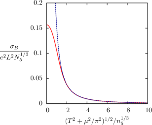
The reason that the current drops as a function of temperature and chemical potential is that in both cases should take a smaller value for a given through Eq. (43). This is because a medium at finite and has fermion distributions with higher momenta that can take part in the chiral charge density. Conversely, a smaller is sufficient to mimic the effect of a given at high temperature/chemical potential, that means that the effect of on systems diminishes by temperature and chemical potential. The generated current decreases accordingly because it is proportional to .
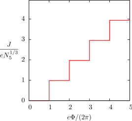
Let us briefly discuss current quantization here. If the size of the magnetic field is large compared to the area in which it is confined the effects of current quantization become important. For example, consider a magnetic field which is constant within a tube with radius and vanishes outside. The effects of current quantization become important if the total flux is comparable to the flux quantum .
In Fig. 3 we have displayed the current as a function of the flux for . Clearly one can see the quantization of the current. If becomes an integer multiple of another zero mode is available, which result in an increase of the current by an amount of .
IV.2 Homogeneous magnetic field
Now let us investigate the current in a strong magnetic field. We now will take a homogeneous field in which we can calculate the induced chiral charge as a function of . Again we start from the thermodynamic potential which in the presence of a homogeneous background magnetic field and a nonzero is given by Eq. (26). Differentiating the thermodynamic potential with respect to gives the chiral charge,
| (50) |
where
| (51) |
In the massless limit the last equation becomes after introducing a cutoff to regularize the integral
| (52) |
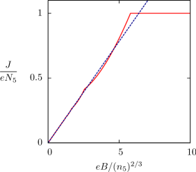
For very large magnetic fields () only the lowest Landau level (only the first term in the brackets) contributes to the current. Hence and the current becomes simply equal to the total chiral charge in the system,
| (53) |
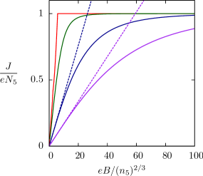
This result can be easily understood from Eq. (11). In a very high magnetic field all modes are fully polarized so that we have . Applying this to Eq. (11) gives Eq. (53) KMW . We shall limit our discussions to the case for a while. If , not only zeroth but also higher order Landau levels start to contribute. In Fig. 4 we have displayed the current calculated numerically as a function of . The current is saturated for . The small magnetic field limit result (45) can be written as
| (54) |
This limit is displayed as well in Fig.4 by a dashed line. The approximation is good as long as the current is not saturated. The slope is
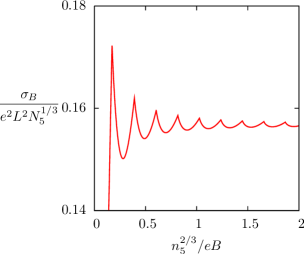
The higher-order Landau levels are creating oscillations in the conductivity through as can be seen from Fig. 5 where we have displayed the conductivity versus . Related oscillations exist in the conductivity induced by an electric field in the presence of a perpendicular magnetic field. In that case they are called Shubnikov–de Haas oscillations. The period of the oscillations is equal to as a function of . Since depends on , the period is not a constant function of . In the small magnetic field limit we can use that . Hence for small magnetic fields the period of the oscillations in the conductivity as a function of becomes . The mean value of the Chiral Magnetic conductivity can be found from the small magnetic field approximation which yields
In order to study the effect of temperature on the current in a homogeneous magnetic field, we have solved Eq. (52) numerically. We have displayed the current in Fig. 6 for different temperatures. Clearly, at higher temperatures it requires larger magnetic fields to saturate the current. This is because at high temperature more higher momentum modes are occupied, which are more difficult to polarize. The dashed lines in Fig. 6 denote the small magnetic field approximations from Eq. (48). On dimensional grounds one expects the small magnetic field approximation to be valid for with . Indeed this can be seen in the figure, at finite temperature the small magnetic field approximation is even good to larger values of the magnetic field than at zero temperature. The oscillations in the Chiral Magnetic conductivity will be smeared by temperature.
IV.3 Implications for heavy-ion collisions
To obtain the induced current in QCD we can sum the previous results over flavors and insert the appropriate color factor. We will give only the high temperature result, since that result will be relatively insensitive to gluonic corrections and is also the most relevant for studying the implications of the topological charge changing transitions in the quark-gluon plasma. Generalizing Eq. (48) we obtain
| (55) |
Here is the electric charge carried by quarks of flavor . Note that in the above is from replacing by . This equation can be used to make predictions for the charge asymmetry in heavy-ion collisions like is done in Ref. KMW . In the quark-gluon plasma we could maybe expect to be several units per deduced from typical QCD sphaleron sizes. In that case . Since at the earliest times just after the collision KMW , ; it follows from Fig. (6) that the current is never expected to be saturated at all. Hence the linear approximation in , Eq. (55), can be applied to the study of the Chiral Magnetic Effect in heavy-ion collisions.
In a heavy-ion collision the magnetic field is pointing along the direction of angular momentum, which is perpendicular to the reaction plane. We can define like in Ref. KMW , to be the difference between the total amount of positive/negative charge above and below the reaction plane in units of . If is small enough we can assume that the probability to produce a quark is the same as anti-quark. Then each time a sphaleron transition with winding number is taking place we find that
| (56) | |||||
| (57) |
The and signs in the equations above should be read as follows. If the winding number is negative (positive), increases (decreases), while decreases (increases). The functions defined in KMW are phenomenological screening functions to describe the effect of the quark-gluon plasma through which the separated particles have to travel.
The observables proposed in Ref. V04 and analyzed in IVS ; VQM are sensitive to the correlators and . These correlators can be obtained from Eqs. (56) and (57) by assuming the one-dimensional random walk picture, folding it with the sphaleron rate and integrating over time and volume. This analysis has been performed in Ref. KMW .
In Ref. KMW the current was estimated to be proportional to the degree of polarization of the quarks with momenta smaller than the inverse size of the typical sphaleron. In Ref. KMW Eqs. (56) and (57) are similar, except that the following replacement has to be made,
| (58) |
Since , where is the strong coupling constant, the newly obtained results are slightly different. The difference stems from the fact that in the calculation in Ref. KMW the typical momenta were determined by the inverse size of the sphaleron, , while in the calculation in this paper, equilibrium was assumed so that the typical momenta are of order .
V Effects of mass and chiral condensate
In the presence of mass right- and left-handed quarks are coupled. A chiral condensate does essentially the same. Because the axial charge density operator does not commute with the Hamiltonian in the presence of a mass term, chirality is not conserved anymore. Hence the massive case becomes a dynamical problem and cannot be studied using the equilibrium approach we used in this article because will depend on time when decays.
The effect of mass on the anomaly was studied in Ref. AGP . It was found that mass term always causes an asymmetry between the number of right- and left-handed fermions to decay. The time-scale of this decay depends the typical momentum (the temperature) of the particles, their mass, and the chiral condensate. For where the momentum scale is much larger than quark masses the decay time will be large, so that the equilibrium approach will be reasonably good. However if the temperature becomes in the neighborhood of the chiral condensate becomes important. Any asymmetry will be washed out, which will reduce the current. It would be very interesting to know how fast the chiral condensate washes out the asymmetry; we will leave this problem for future study.
VI The chiral battery
We would like to point out an interesting hypothetical application of the Chiral Magnetic Effect – a rechargeable battery which stores chirality – the chiral battery.
Let us imagine a hypothetical material with charged fermion quasi-particles described by the massless Dirac equation. In this Dirac equation the velocity of light is to be replaced by the much smaller Fermi velocity of the quasi-particles. A recent example of such a material is provided by graphene (for a review see e.g. graphene ), even though we should keep in mind that chirality in graphene is not related to the ”usual” spin states considered above but instead refers to the sub-lattice states. More directly, our considerations may apply to zero-gap semiconductors with the linear dispersion relation – possibly, tellurides.
If we have some finite amount of this material, it can be used as a battery. The battery can be charged using the axial anomaly by placing it in parallel electric and magnetic fields. The charging time will be determined by the axial anomaly. The battery stores energy, since the Fermi-levels of right- and left-handed modes differ. In a sense, this material is also to be regarded as “chiral capacitor.”
In the absence of electric and magnetic fields, chirality is conserved, so the battery does not discharge. Now let us connect the battery to a circuit element with resistance . If we apply a magnetic field to the battery in the right direction, a current will be induced due to the Chiral Magnetic Effect. Note that the magnetic field alone does no work on fermions in the battery. The behavior of this current as a function of the applied magnetic field and temperature will follow from our analysis in Sec. III. The current will cause a potential difference over the circuit element. As a result, the same potential difference will also exist over the battery. Hence an electric field will arise parallel to the magnetic field. In this case the axial anomaly operates again to decrease the chirality. Hence the rate of discharge will be determined by the axial anomaly as well.
Let us estimate the amount of energy stored in the chiral battery per unit volume. It is equal to the Helmholtz free energy, which is the energy that can be used to do work. The free energy is the difference between the thermodynamic potential with a chiral charge density and without and is easily found by integrating Eq. (43) with respect to .
We then obtain
| (59) |
At zero temperature and chemical potential we can use Eq. (43) to express in terms of the chiral charge density. We find
| (60) |
The typical distance between the lattice sites in a crystal is of order . Suppose we can store unit of chirality per lattice site, i.e. an excess of 100 right-handed fermions over left-handed fermions per . Then the energy density will be
| (61) |
Here is the Fermi velocity. In typical materials like graphene , so the typical storage capacity of the chiral battery is of order . This is comparable or better than ”conventional” batteries whose energy density is typically ; note besides that the current in our case is spin-polarized and so may be used for spintronic applications.
VII Conclusions
A system with a nonzero chirality responds to a magnetic field by inducing a current along the magnetic field. This is the Chiral Magnetic Effect. The behavior of the current as a function of chirality, baryon chemical potential and temperature has been obtained in equilibrium in this article.
The Chiral Magnetic Effect can be studied using heavy-ion collisions. The possible experimental observation of the Chiral Magnetic Effect would be direct evidence for the existence and relevance of gluon configurations with non-trivial topology. Furthermore it will signal - and -violation in QCD on an event-by-event basis. A thorough theoretical understanding of the Chiral Magnetic Effect will help the experimental analysis by offering the possibility of more accurate predictions of the observables.
Since the Chiral Magnetic Effect is due to a mixture of QCD and electromagnetic effects, it has very characteristic behavior. For example it is expected that the correlators analyzed in experiment are proportional to the square of the charge of the colliding nuclei. This very specific behavior can be investigated by measuring collisions of nuclei with the same atomic number but different charge. With better theoretical understanding, more predictions could be made.
The Chiral Magnetic Effect can only operate in the deconfined, chirally symmetric phase. Deconfinement is necessary, because quarks need to be separated over long distances in order for the Chiral Magnetic Effect to work. Restoration of chiral symmetry is needed, since a chiral condensate always will wash out any difference between the number of right- and left-handed quarks. Hence if observed the Chiral Magnetic Effect might be used as an order parameter for the confinement/deconfinement and the chiral symmetry breakdown/restoration transition.
Because the Chiral Magnetic Effect probes the - and -violating interactions in QCD it can help us to get a better understanding of the so-called strong problem. The problem refers to the fact that strong interactions do not break the and symmetries explicitly even though an addition of – and –odd -term to the QCD Lagrangian is perfectly allowed without spoiling gauge invariance. The Chiral Magnetic Effect probes the configurations which in principle also cause explicit - and violation if is non-vanishing.
The Chiral Magnetic Effect has also a nice analogy in the physics of the Early Universe. One mechanism to explain the matter-antimatter asymmetry is electroweak baryogenesis KRS ; Shaposhnikov1987 . There electroweak sphalerons induce via the axial anomaly - and -odd effects. As a result baryon plus lepton number is generated. This process is very similar to the Chiral Magnetic Effect. It is also quite possible that the Chiral Magnetic Effect itself could have an important role in the Early Universe if a large magnetic field and/or a non-zero expectation value of the axion field were present at that time.
Acknowledgments
We are grateful to Larry McLerran and Eric Zhitnitsky for discussions; we thank Larry McLerran also for comments on the manuscript.
This manuscript has been authored under Contract No. #DE-AC02-98CH10886 with the U.S. Department of Energy. K. F. is supported by Japanese MEXT grant no. 20740134 and also supported in part by Yukawa International Program for Quark Hadron Sciences.
References
- (1) A. A. Belavin, A. M. Polyakov, A. S. Shvarts and Yu. S. Tyupkin, Phys. Lett. B 59, 85 (1975).
- (2) G. ’t Hooft, Phys. Rev. Lett. 37, 8 (1976); G. ’t Hooft, Phys. Rev. D 14, 3432 (1976).
- (3) E. Witten, Nucl. Phys. B 156, 269 (1979); G. Veneziano, Nucl. Phys. B 159, 213 (1979).
- (4) G. ’t Hooft, Phys. Rept. 142, 357 (1986).
- (5) M. C. Chu, J. M. Grandy, S. Huang and J. W. Negele, Phys. Rev. D 49, 6039 (1994); C. Michael and P. S. Spencer, Phys. Rev. D 52, 4691 (1995).
- (6) D. J. Gross, R. D. Pisarski and L. G. Yaffe, Rev. Mod. Phys. 53, 43 (1981).
- (7) T. Schafer and E. V. Shuryak, Rev. Mod. Phys. 70, 323 (1998).
- (8) N. S. Manton, Phys. Rev. D 28, 2019 (1983).
- (9) F. R. Klinkhamer and N. S. Manton, Phys. Rev. D 30, 2212 (1984).
- (10) V. A. Kuzmin, V. A. Rubakov and M. E. Shaposhnikov, Phys. Lett. B 155, 36 (1985).
- (11) P. Arnold and L. D. McLerran, Phys. Rev. D 36, 581 (1987).
- (12) S. Y. Khlebnikov and M. E. Shaposhnikov, Nucl. Phys. B 308, 885 (1988).
- (13) P. Arnold and L. D. McLerran, Phys. Rev. D 37, 1020 (1988).
- (14) M. E. Shaposhnikov, Nucl. Phys. B 287, 757 (1987).
- (15) L. D. McLerran, E. Mottola and M. E. Shaposhnikov, Phys. Rev. D 43, 2027 (1991).
- (16) G. F. Giudice and M. E. Shaposhnikov, Phys. Lett. B 326, 118 (1994).
- (17) E. Shuryak and I. Zahed, Phys. Rev. D 67, 014006 (2003).
- (18) G. D. Moore, Phys. Lett. B 412, 359 (1997); G. D. Moore and K. Rummukainen, Phys. Rev. D 61, 105008 (2000); D. Bödeker, G. D. Moore and K. Rummukainen, Phys. Rev. D 61, 056003 (2000); G. D. Moore, arXiv:hep-ph/0009161.
- (19) S. L. Adler, Phys. Rev. 177, 2246 (1969); J. S. Bell and and R. Jackiw, Nuovo Cim. A60, 47 (1969).
- (20) N. H. Christ, Phys. Rev. D 21, 1591 (1980).
- (21) A. V. Smilga, Phys. Rev. D 45, 1378 (1992).
- (22) J. Ambjorn, J. Greensite and C. Peterson, Nucl. Phys. B 221, 381 (1983).
- (23) D. Kharzeev, A. Krasnitz and R. Venugopalan, Phys. Lett. B 545, 298 (2002).
- (24) T. Lappi and L. McLerran, Nucl. Phys. A 772, 200 (2006).
- (25) D. E. Kharzeev, Y. V. Kovchegov and E. Levin, Nucl. Phys. A 699, 745 (2002); Nucl. Phys. A 690, 621 (2001); D. Kharzeev, E. Levin and K. Tuchin, Phys. Rev. C 75, 044903 (2007).
- (26) P. Romatschke and R. Venugopalan, Phys. Rev. Lett. 96, 062302 (2006); Phys. Rev. D 74, 045011 (2006).
- (27) D. Kharzeev, Phys. Lett. B 633, 260 (2006).
- (28) D. Kharzeev and A. Zhitnitsky, Nucl. Phys. A 797, 67 (2007).
- (29) D. E. Kharzeev, L. D. McLerran and H. J. Warringa, Nucl. Phys. A 803, 227 (2008).
- (30) H. J. Warringa, arXiv:0805.1384 [hep-ph].
- (31) S. A. Voloshin, Phys. Rev. C 70, 057901 (2004).
- (32) I. V. Selyuzhenkov [STAR Collaboration], Rom. Rep. Phys. 58, 049 (2006).
- (33) S. A. Voloshin [STAR Collaboration], arXiv:0806.0029 [nucl-ex].
- (34) V. P. Gusynin, V. A. Miransky and I. A. Shovkovy, Phys. Rev. D 52, 4747 (1995).
- (35) I. A. Shushpanov and A. V. Smilga, Phys. Lett. B 402, 351 (1997).
- (36) T. D. Cohen, D. A. McGady and E. S. Werbos, Phys. Rev. C 76, 055201 (2007).
- (37) E. S. Fraga and A. J. Mizher, Phys. Rev. D 78, 025016 (2008).
- (38) N. O. Agasian and S. M. Fedorov, Phys. Lett. B 663, 445 (2008).
- (39) M. G. Alford, J. Berges and K. Rajagopal, Nucl. Phys. B 571, 269 (2000).
- (40) E. J. Ferrer, V. de la Incera and C. Manuel, Phys. Rev. Lett. 95, 152002 (2005).
- (41) K. Fukushima and H. J. Warringa, Phys. Rev. Lett. 100, 032007 (2008).
- (42) J. L. Noronha and I. A. Shovkovy, Phys. Rev. D 76, 105030 (2007).
- (43) D. T. Son and A. R. Zhitnitsky, Phys. Rev. D 70, 074018 (2004).
- (44) M. A. Metlitski and A. R. Zhitnitsky, Phys. Rev. D 72, 045011 (2005).
- (45) D. T. Son and M. A. Stephanov, Phys. Rev. D 77, 014021 (2008).
- (46) H. B. Nielsen and M. Ninomiya, Phys. Lett. B 130, 389 (1983).
- (47) E. Witten, Nucl. Phys. B 249, 557 (1985).
- (48) D. Kharzeev, R. D. Pisarski and M. H. G. Tytgat, Phys. Rev. Lett. 81, 512 (1998); arXiv:hep-ph/0012012.
- (49) T. Fugleberg, I. E. Halperin and A. Zhitnitsky, Phys. Rev. D 59, 074023 (1999) R. H. Brandenberger, I. E. Halperin and A. Zhitnitsky, arXiv:hep-ph/9808471; K. Buckley, T. Fugleberg and A. Zhitnitsky, Phys. Rev. Lett. 84, 4814 (2000) D. Ahrensmeier, R. Baier and M. Dirks, Phys. Lett. B 484, 58 (2000); E. V. Shuryak and A. R. Zhitnitsky, Phys. Rev. C 66, 034905 (2002); A. K. Chaudhuri, Phys. Rev. C 65, 024906 (2002); M. Creutz, Phys. Rev. Lett. 92, 201601 (2004); arXiv:hep-ph/0312225; E. Vicari and H. Panagopoulos, arXiv:0803.1593 [hep-th]; D. Boer and J. K. Boomsma, arXiv:0806.1669 [hep-ph].
- (50) A. N. Sisakian, O. Y. Shevchenko and S. B. Solganik, arXiv:hep-th/9806047.
- (51) M. Joyce, T. Prokopec and N. Turok, Phys. Rev. D 53, 2958 (1996).
- (52) Y. Aharonov and A. Casher Phys. Rev. A 19, 2461 (1979).
- (53) E. D’Hoker and J. Goldstone, Phys. Lett. B 158, 429 (1985).
- (54) R. D. Ball and H. Osborn, Phys. Lett. B 165, 410 (1985).
- (55) J. Goldstone and F. Wilczek, Phys. Rev. Lett. 47, 986 (1981).
- (56) C. G. Callan and J. A. Harvey, Nucl. Phys. B 250, 427 (1985).
- (57) D. Boyanovsky, E. Dagotto and E. H. Fradkin, Nucl. Phys. B 285, 340 (1987).
- (58) E. H. Fradkin, E. Dagotto and D. Boyanovsky, Phys. Rev. Lett. 57, 2967 (1986) [Erratum-ibid. 58, 961 (1987)].
- (59) K. S. Novoselov, A. K. Geim, S. V. Morosov, D. Jiang, M. I. Katsnelson, I. V. Grigorieva, S. V. Dubonos, and A. A. Firsov, Nature (London) 438, 197 (2005); A. K. Geim and K. S. Novoselov, Nature Materials 6, 183 (2007); A. H. Castro Neto, F. Guinea, N. M. R. Peres, K. S. Novoselov, A. K. Geim, arXiv:0709.1163 [cond-mat.other].