Equilibrium and traveling-wave solutions of plane Couette flow
We present ten new equilibrium solutions to plane Couette flow in small periodic cells at low Reynolds number Re and two new traveling-wave solutions. The solutions are continued under changes of Re and spanwise period. We provide a partial classification of the isotropy groups of plane Couette flow and show which kinds of solutions are allowed by each isotropy group. We find two complementary visualizations particularly revealing. Suitably chosen sections of their -physical space velocity fields are helpful in developing physical intuition about coherent structures observed in low Re turbulence. Projections of these solutions and their unstable manifolds from their -dimensional state space onto suitably chosen 2- or 3-dimensional subspaces reveal their interrelations and the role they play in organizing turbulence in wall-bounded shear flows.
1 Introduction
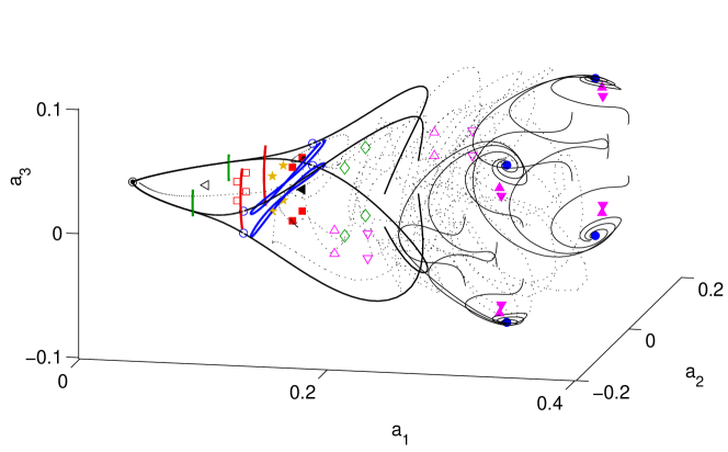
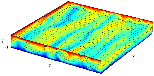
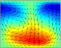
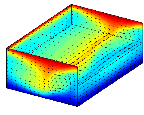
In Gibson et al. (2008) (henceforth referred to as GHC) we formed visualizations of the -dimensional state-space dynamics of moderate Re turbulent flows, using precisely calculated equilibrium solutions of the Navier-Stokes equations to define dynamically invariant, intrinsic, and representation independent coordinate frames. These state-space portraits (figure 1) offer a visualization of the dynamics of transitionally turbulent flows, complementary to visualizations of the spatial features of velocity fields (figure 2). Side-by-side animations of the two visualizations illustrate their complementary strengths (see Gibson (2008b) online simulations). In these animations, spatial visualization of instantaneous velocity fields helps elucidate the physical processes underlying the formation of unstable coherent structures, such as the Self-Sustained Process (SSP) theory of Waleffe (1990, 1995, 1997). Running concurrently, the -dimensional state-space representation enables us to track the unstable manifolds of equilibria and the heteroclinic connections between them (Halcrow et al., 2009), and provides us with new insight into the nonlinear state space geometry and dynamics of moderate Re wall-bounded flows.
Here we continue our investigation of equilibrium and traveling-wave solutions of Navier-Stokes equations, presenting ten new equilibrium solutions and two new traveling waves of plane Couette flow, and continuing the solutions as functions of Re and periodic cell size . Nagata found the first pair of nontrivial equilibria (Nagata, 1990) and the first traveling wave in plane Couette flow (Nagata, 1997). Clever & Busse (1992) found closely related equilibria in plane Couette flow with Rayleigh-Bénard convection. Cherhabili & Ehrenstein (1997) reported two-dimensional equilibria of plane Couette but these were later shown to be artifacts of the truncation (Rincon, 2007; Ehrenstein et al., 2008). Waleffe (1998, 2003) computed the Nagata equilibria guided by the SSP theory and showed that they were insensitive to the boundary conditions at the wall. Other traveling waves were computed by Viswanath (2008) and Jiménez et al. (2005). Schmiegel (1999) computed and investigated a large number of equilibria. His 1999 Ph.D. provides a wealth of ideas and information on solutions to plane Couette flow, and in many regards the published literature is still catching up this work. GHC added the dynamically important equilibrium (labeled in this paper). Parallel theoretical advances have been made in channel and pipe flows, with the discovery of traveling waves in channel flows (Waleffe, 2001), and traveling waves (Faisst & Eckhardt, 2003; Wedin & Kerswell, 2004; Pringle & Kerswell, 2007) and relative periodic orbits (Duguet et al., 2008) in pipes. Moreover, traveling waves have been observed experimentally in turbulent pipe flow (Hof et al., 2004). We refer the reader to GHC for a more detailed review.
We review plane Couette flow in § 2. The main advances reported in this paper are (§ 3) a classification of plane Couette symmetry groups that support equilibria, (§ 4) the determination of a number of new equilibria and traveling waves of plane Couette flow, and (§ 5, § 6) continuation of these solutions in Reynolds number and spanwise aspect ratio. Outstanding challenges are discussed in § 7. Detailed numerical results such as stability eigenvalues and symmetries of corresponding eigenfunctions are given in Halcrow (2008), while the complete data sets for the invariant solutions can be downloaded from channelflow.org.
2 Plane Couette flow – a review
Plane Couette flow is comprised of an incompressible viscous fluid confined between two infinite parallel plates moving in opposite directions at constant velocities, with no-slip boundary conditions imposed at the walls. The plates move along the streamwise or direction, the wall-normal direction is , and the spanwise direction is . The fluid velocity field is . We define the Reynolds number as , where is half the relative velocity of the plates, is half the distance between the plates, and is the kinematic viscosity. After non-dimensionalization, the plates are positioned at and move with velocities , and the Navier-Stokes equations are
| (1) |
We seek spatially periodic equilibrium and traveling-wave solutions to (1) for the domain (or ), with periodic boundary conditions in and . Equivalently, the spatial periodicity of solutions can be specified in terms of their fundamental wavenumbers and . A given solution is compatible with a given domain if and for integer . In this study the spatial mean of the pressure gradient is held fixed at zero.
Most of this study is conducted at in one of the two small aspect-ratio cells
| (2) |
where the wall units are in relation to a mean shear rate of in non-dimensionalized units computed for a large aspect-ratio simulation at . Empirically, at this Reynolds number the cell sustains turbulence for very long times (Hamilton et al., 1995), whereas the cell exhibits only short-lived transient turbulence (GHC). The length scale of was chosen as a compromise between the of and its first harmonic (Waleffe, 2002). Unless stated otherwise, all calculations are carried out for and the cell. In the notation of this paper, the solutions presented in Nagata (1990) have wavenumbers and fit in the cell .111Note also that Reynolds number in Nagata (1990) is based on the full wall separation and the relative wall velocity, making it a factor of four larger than the Reynolds number used in this paper. Waleffe (2003) showed that these solutions first appear at critical Reynolds number of 127.7 and . Schmiegel (1999)’s study of plane Couette solutions and their bifurcations was conducted in the cell of size .
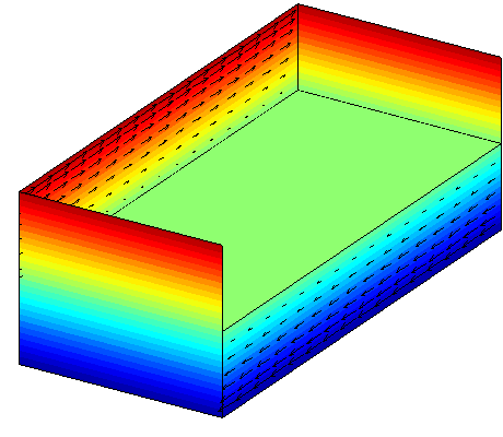
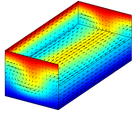
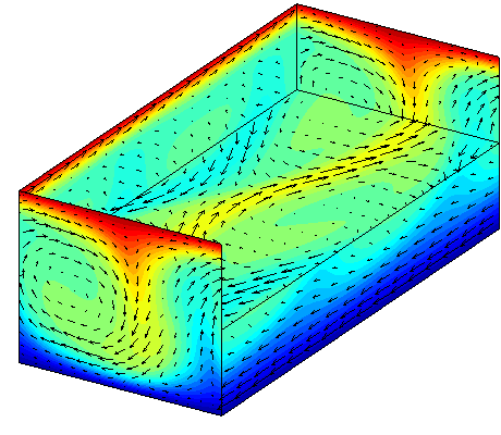
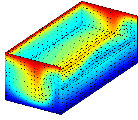
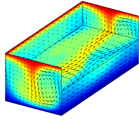
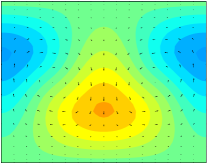
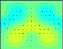
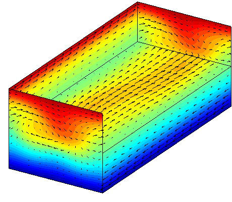
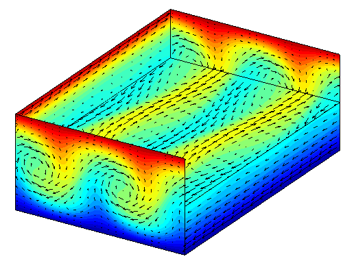
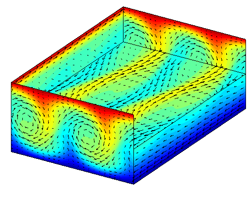
Although the aspect ratios studied in this paper are small, the states explored by equilibria and their unstable manifolds explored here are strikingly similar to typical states in larger aspect-ratio cells, such as figure 2. Kim et al. (1971) observed that streamwise instabilities give rise to pairwise counter-rotating rolls whose spanwise separation is approximately 100 wall units. These rolls, in turn, generate streamwise streaks of high and low speed fluid, by convecting fluid alternately away from and towards the walls. The streaks have streamwise instabilities whose length scale is roughly twice the roll separation. These ‘coherent structures’ are prominent in numerical and experimental observations (see figure 2 and Gibson (2008b) animations), and they motivate our investigation of how equilibrium and traveling-wave solutions of Navier-Stokes change with Re and cell size.
Fluid states are characterized by their energy and energy dissipation rate , defined in terms of the inner product and norm
| (3) |
The rate of energy input is , where the integral is taken over the upper and lower walls at . Normalization of these quantities is set so that for laminar flow and . It is often convenient to consider fields as differences from the laminar flow, since these differences constitute a vector space, and thus can be added together, multiplied by scalars, etc. We indicate such differences with tildes: . Note that the total velocity field does not form a vector space: the sum of any two total plane Couette velocity fields violates the boundary conditions at the moving walls.
3 Symmetries and isotropy subgroups
On an infinite domain and in the absence of boundary conditions, the Navier-Stokes equations are equivariant under any translation, rotation, and , inversion through the origin (Frisch, 1996). In plane Couette flow, the counter-moving walls restrict the rotation symmetry to rotation by about the -axis. We denote this rotation by and the inversion through the origin by . The suffixes indicate which of the homogeneous directions change sign and simplify the notation for the group algebra of rotation, inversion, and translations presented in § 3.1 and § 3.2. The and symmetries generate a discrete dihedral group of order 4, where
| (4) | ||||
The walls also restrict the translation symmetry to in-plane translations. With periodic boundary conditions, these translations become the continuous two-parameter group of streamwise-spanwise translations
| (5) |
The equations of plane Couette flow are thus equivariant under the group , where stands for a semi-direct product, subscripts indicate streamwise translations and sign changes in , and subscripts indicate spanwise translations and sign changes in .
The solutions of an equivariant system can satisfy all of the system’s symmetries, a proper subgroup of them, or have no symmetry at all. For a given solution , the subgroup that contains all symmetries that fix (that satisfy ) is called the isotropy (or stabilizer) subgroup of . (Hoyle, 2006; Marsden & Ratiu, 1999; Golubitsky & Stewart, 2002; Gilmore & Letellier, 2007). For example, a typical turbulent trajectory has no symmetry beyond the identity, so its isotropy group is . At the other extreme is the laminar equilibrium, whose isotropy group is the full plane Couette symmetry group .
In between, the isotropy subgroup of the Nagata equilibria and most of the equilibria reported here is , where
| (6) | ||||
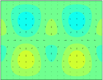
These particular combinations of flips and shifts match the symmetries of instabilities of streamwise-constant streaky flow (Waleffe, 1997, 2003) and are well suited to the wavy streamwise streaks observable in figure 2, with suitable choice of and . But is one choice among a number of intermediate isotropy groups of , and other subgroups might also play an important role in the turbulent dynamics. In this section we provide a partial classification of the isotropy groups of , sufficient to classify all currently known invariant solutions and to guide the search for new solutions with other symmetries. We focus on isotropy groups involving at most half-cell shifts. The main result is that among these, up to conjugacy in spatial translation, there are only five isotropy groups in which we should expect to find equilibria.
3.1 Flips and half-shifts
A few observations will be useful in what follows. First, we note the key role played by the rotation and reflection symmetries and (4) in the classification of solutions and their isotropy groups. The equivariance of plane Couette flow under continuous translations allows for traveling-wave solutions, i.e., solutions that are steady in a frame moving with a constant velocity in . In state space, traveling waves either trace out circles or wind around tori, and these sets are both continuous-translation and time invariant. The sign changes under , , and , however, imply particular centers of symmetry in , , and both and , respectively, and thus fix the translational phases of fields that are fixed by these symmetries. Thus the presence of or in an isotropy group prohibits traveling waves in or , and the presence of prohibits any form of traveling wave. Guided by this observation, we will seek equilibria only for isotropy subgroups that contain the inversion symmetry.
Second, the periodic boundary conditions impose discrete translation symmetries of and on velocity fields. In addition to this full-period translation symmetry, a solution can also be fixed under a rational translation, such as or a continuous translation . If a field is fixed under continuous translation, it is constant along the given spatial variable. If it is fixed under rational translation , it is fixed under for as well, provided that and are relatively prime. For this reason the subgroups of the continuous translation consist of the discrete cyclic groups for together with the trivial subgroup and the full group itself, and similarly for . For rational shifts we simplify the notation a bit by rewriting (5) as
| (7) |
Since will loom large in what follows, we omit exponents of :
| (8) |
If a field is fixed under a rational shift , it is periodic on the smaller spatial domain . For this reason we can exclude from our searches all equilibrium whose isotropy subgroups contain rational translations in favor of equilibria computed on smaller domains. However, as we need to study bifurcations into states with wavelengths longer than the initial state, the linear stability computations need to be carried out in the full cell. For example, if EQ is an equilibrium solution in the cell, we refer to the same solution repeated thrice in as “spanwise-tripled” or . Such solution is by construction fixed under the subgroup.
Third, some isotropy groups are conjugate to each other under symmetries of the full group . Subgroup is conjugate to if there is an for which . In spatial terms, two conjugate isotropy groups are equivalent to each other under a coordinate transformation. A set of conjugate isotropy groups forms a conjugacy class. It is necessary to consider only a single representative of each conjugacy class; solutions belonging to conjugate isotropy groups can be generated by applying the symmetry operation of the conjugacy.
In the present case conjugacies under spatial translation symmetries are particularly important. Note that is not an abelian group, since reflections and translations along the same axis do not commute (Harter, 1993). Instead we have . Rewriting this relation as , we note that
| (9) |
The right-hand side of (9) is a similarity transformation that translates the origin of coordinate system. For we have
| (10) |
and similarly for the spanwise shifts / reflections. Thus for each isotropy group containing the shift-reflect symmetry, there is a simpler conjugate isotropy group in which is replaced by (and similarly for and ). We choose as the representative of each conjugacy class the simplest isotropy group, in which all such reductions have been made. However, if an isotropy group contains both and , it cannot be simplified this way, since the conjugacy simply interchanges the elements.
Fourth, for , we have so that, in the special case of half-cell shifts, and commute. For the same reason, and commute, so the order-16 isotropy subgroup
| (11) |
is abelian.
3.2 The 67-fold path
We now undertake a partial classification of the lattice of isotropy subgroups of plane Couette flow. We focus on isotropy groups involving at most half-cell shifts, with translations restricted to order 4 subgroup of spanwise-streamwise translations (8) of half the cell length,
| (12) |
All such isotropy subgroups of are contained in the subgroup (11). Within , we look for the simplest representative of each conjugacy class, as described above.
Let us first enumerate all subgroups . The subgroups can be of order . A subgroup is generated by multiplication of a set of generator elements, with the choice of generator elements unique up to a permutation of subgroup elements. A subgroup of order has only one generator, since every group element is its own inverse. There are 15 non-identity elements in to choose from, so there are 15 subgroups of order 2. Subgroups of order 4 are generated by multiplication of two group elements. There are 15 choices for the first and 14 choices for the second. However, each order-4 subgroup can be generated by different choices of generators. For example, any two of in any order generate the same group . Thus there are subgroups of order 4.
Subgroups of order 8 have three generators. There are 15 choices for the first generator, 14 for the second, and 12 for the third. There are 12 choices for the third generator and not 13, since if it were chosen to be the product of the first two generators, we would get a subgroup of order 4. Each order-8 subgroup can be generated by different choices of three generators, so there are subgroups of order 8. In summary: there is the group itself, of order 16, 15 subgroups of order 8, 35 of order 4, 15 of order 2, and 1 (the identity) of order 1, or 67 subgroups in all (Halcrow, 2008). This is whole lot of isotropy subgroups to juggle; fortunately, the observations of § 3.1 show that there are only 5 distinct conjugacy classes in which we can expect to find equilibria.
The 15 order-2 groups fall into 8 distinct conjugacy classes, under conjugacies between and and and . These conjugacy classes are represented by the 8 isotropy groups generated individually by the 8 generators and . Of these, the latter three imply periodicity on smaller domains. Of the remaining five, and allow traveling waves in , and allow traveling waves in . Only a single conjugacy class, represented by the isotropy group
| (13) |
breaks both continuous translation symmetries. Thus, of all order-2 isotropy groups, we expect only this group to have equilibria. , , and described below are examples of equilibria with isotropy group .
Of the 35 subgroups of order 4, we need to identify those that contain and thus support equilibria. We choose as the simplest representative of each conjugacy class the isotropy group in which appears in isolation. Four isotropy subgroups of order 4 are generated by picking as the first generator, and or as the second generator (R for reflect-rotate):
| (14) | ||||
These are the only isotropy groups of order 4 containing and no isolated translation elements. Together with , these 5 isotropy subgroups represent the 5 conjugacy classes in which expect to find equilibria.
The isotropy subgroup is particularly important, as the Nagata (1990) equilibria belong to this conjugacy class (Waleffe, 1997; Clever & Busse, 1997; Waleffe, 2003), as do most of the solutions reported here. The NBC isotropy subgroup of Schmiegel (1999) and of Gibson et al. (2008) are conjugate to under quarter-cell coordinate transformations. In keeping with previous literature, we often represent this conjugacy class with rather than the simpler conjugate group . Schmiegel’s I isotropy group is conjugate to our ; Schmiegel (1999) contains many examples of -isotropic equilibria. -isotropic equilibria were found by Tuckerman & Barkley (2002) for plane Couette flow in which the translation symmetries were broken by a streamwise ribbon. We have not searched for -isotropic solutions, and are not aware of any published in the literature.
The remaining subgroups of orders 4 and 8 all involve factors and thus involve states that are periodic on half-domains. For example, the isotropy subgroup of and studied below is , and thus these are doubled states of solutions on half-domains. For the detailed count of all 67 subgroups, see Halcrow (2008).
3.3 State-space visualization
GHC presents a method for visualizing low-dimensional projections of trajectories in the infinite-dimensional state space of the Navier-Stokes equations. Briefly, we construct an orthonormal basis that spans a set of physically important fluid states , , , such as equilibrium states and their eigenvectors, and we project the evolving fluid state onto this basis using the inner product (3). This produces a low-dimensional projection
| (15) |
which can be viewed in planes or in perspective views . The state-space portraits are dynamically intrinsic, since the projections are defined in terms of intrinsic solutions of the equations of motion, and representation independent, since the inner product (3) projection is independent of the numerical or experimental representation of the fluid state data. Such bases are effective because moderate-Re turbulence explores a small repertoire of unstable coherent structures (rolls, streaks, their mergers), so that the trajectory does not stray far from the subspace spanned by the key structures.
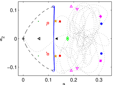
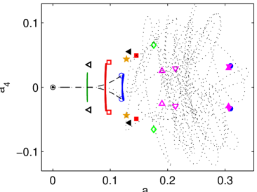
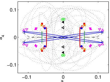
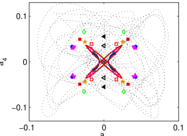
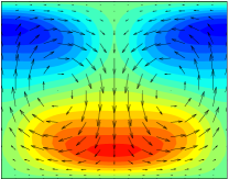
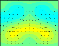
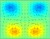
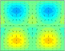
There is no a priori prescription for picking a ‘good’ set of basis fluid states, and construction of set requires some experimentation. Let the -invariant subspace be the flow-invariant subspace of states that are fixed under ; this consists of all states whose isotropy group is or contains as a subgroup. The plane Couette system at hand has a total of 29 known equilibria within the -invariant subspace: four translated copies each of - , two translated copies of (which have an additional symmetry), plus the laminar equilibrium at the origin. As shown in GHC, the dynamics of different regions of state space can be elucidated by projections onto basis sets constructed from combinations of equilibria and their eigenvectors.
In this paper we present global views of all invariant solutions in terms of the orthonormal ‘translational basis’ constructed in GHC from the four translated copies of :
| (16) | ||||
where is a normalization constant determined by . The last 3 columns indicate the symmetry of the basis vector under half-cell translations; e.g. in the column implies .
4 Equilibria and traveling waves of plane Couette flow
We seek equilibrium solutions to (1) of the form and traveling-wave or relative equilibrium solutions of the form with . Let represent the Navier-Stokes equations (1) for the given geometry, boundary conditions, and Reynolds number, and its time- forward map
| (17) |
Then for any fixed , equilibria satisfy and traveling waves satisfy , where . When is approximated with a finite spectral expansion and with a numerical simulation algorithm, these equations become a set of nonlinear equations in the expansion coefficients for and, in the case of traveling waves, the wave velocities .
Viswanath (2007) presents an algorithm for computing solutions to these equations based on Newton search, Krylov subspace methods, and an adaptive ‘hookstep’ trust-region limitation to the Newton steps. This algorithm can provide highly accurate solutions from even poor initial guesses. The high accuracy stems from the use of Krylov subspace methods, which can be efficient with or more spectral expansion coefficients. The robustness with respect to initial guess stems from the hookstep algorithm. The hookstep limitation restricts steps to a radius of estimated validity for the local linear approximation to the Newton equations. As increases from zero, the direction of the hookstep varies smoothly from the gradient of the residual within the Krylov subspace to the Newton step, so that the hookstep algorithm behaves as a gradient descent when far away from a solution and as the Newton method when near, thus greatly increasing the algorithm’s region of convergence around solutions, compared to the Newton method (J.E. Dennis, Jr., & Schnabel, 1996).
The choice of initial guesses for the search algorithm is one of the main differences between this study and previous calculations of equilibria and traveling waves of shear flows. Prior studies have used homotopy, that is, starting from a solution to a closely related problem and following it through small steps in parameter space to the problem of interest. Equilibria for plane Couette flow have been continued from Taylor-Couette flow (Nagata, 1990), Rayleigh-Bénard flow (Clever & Busse, 1997), and from plane Couette with imposed body forces (Waleffe, 1998). Equilibria and traveling waves have also been found using “edge-tracking” algorithms, that is, by adjusting the magnitude of a perturbation of the laminar flow until it neither decays to laminar nor grows to turbulence, but instead converges toward a nearby weakly unstable solution (Itano & Toh (2001); Skufca et al. (2006); Viswanath (2008); Schneider et al. (2008)). In this study, we take as initial guesses samples of velocity fields generated by long-time simulations of turbulent dynamics. The intent is to find the dynamically most important solutions, by sampling the turbulent flow’s natural measure.
We discretize with a spectral expansion of the form
| (18) |
where the are Chebyshev polynomials. Time integration of is performed with a primitive-variables Chebyshev-tau algorithm with tau correction, influence-matrix enforcement of boundary conditions, and third-order semi-implicit backwards-differentiation time stepping, and dealiasing in and (Kleiser & Schumann (1980); Canuto et al. (1988); Peyret (2002)). We eliminate from the search space the linearly dependent spectral coefficients of that arise from incompressibility, boundary conditions, and complex conjugacies that arise from the real-valuedness of velocity fields. Our codes for Navier-Stokes integration, Newton-hookstep search, parametric continuation, and eigenvalue calculation are available for download from channelflow.org website (Gibson, 2008a), along with a database of all solutions described in this paper. For further details on the numerical methods see GHC and Halcrow (2008).
Solutions presented in this paper use spatial discretization (18) with (or gridpoints) and roughly 60k expansion coefficients, and integration is performed with a time step of . The estimated accuracy of each solution is listed in table 1. As is clear from Schmiegel (1999) Ph.D. thesis, ours is almost certainly an incomplete inventory; while for any finite Re, finite aspect-ratio cell the number of distinct equilibrium and traveling wave solutions is finite, we know of no way of determining or bounding this number. It is difficult to compare our solutions directly to those of Schmiegel since those solutions were computed in a cell (roughly twice our cell size in both span and streamwise directions) and with lower spatial resolution (2212 independent expansion functions versus our 60k for a cell of one-fourth the volume).
4.1 Equilibrium solutions
Our primary focus is on the -invariant subspace (6) of the cell at . We initiated 28 equilibrium searches at evenly spaced intervals along a trajectory in the unstable manifold of that exhibited turbulent dynamics for 800 nondimensionalized time units after leaving the neighborhood of and before decaying to laminar flow. Lower, upper branch pairs are labeled with consecutive numbers, and the numbers indicate, as closely as possible, the order of discovery. We give a name to any distinct solution in the cell at , although many of these solutions can be connected by continuation in Re or wavenumber. is the laminar equilibrium, and are the Nagata lower and upper branch, and is the solution reported in GHC. The rest are new. Only one of the 28 searches failed to converge onto an equilibrium; the successful searches converged to equilibria with frequencies listed in table 1. The higher frequency of occurrence of and suggests that these are the dynamically most important equilibria in the -invariant subspace for the cell at . Stability eigenvalues of known equilibria are plotted in figure 7. Tables of stability eigenvalues and other properties of these solutions are given in Halcrow (2008), while the images, movies and full data sets are available online at channelflow.org. All equilibrium solutions have zero spatial-mean pressure gradient, which was imposed in the flow conditions, and, due to their symmetry, zero mean velocity.
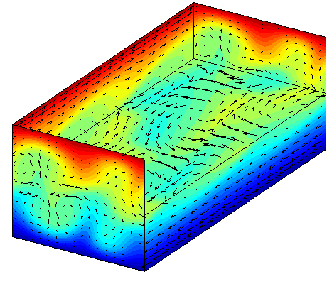


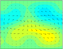
, equilibria. This pair of solutions was discovered by Nagata (1990), recomputed by different methods by Clever & Busse (1992, 1997) and Waleffe (1998, 2003), and found multiple times in searches initiated from turbulent simulation data, as described above. The lower branch and the upper branch are born together in a saddle-node bifurcation at . Just above bifurcation, the two equilibria are connected by a heteroclinic connection, see Halcrow et al. (2009). However, at higher values of Re there appears to be no such simple connection. The lower branch equilibrium is discussed in detail in Wang et al. (2007). This equilibrium has a 1-dimensional unstable manifold for a wide range of parameters. Its stable manifold appears to provide a partial barrier between the basin of attraction of the laminar state and turbulent states (Schneider et al., 2008). The upper branch has an 8-dimensional unstable manifold and a dissipation rate that is higher than the turbulent mean, see figure 8 (a). However, within the -invariant subspace has just one pair of unstable complex eigenvalues. The two-dimensional -invariant section of its unstable manifold was explored in some detail in GHC. It appears to bracket the upper end of turbulence in state space, as illustrated by figure 1.
, . The upper branch solution was found in GHC and is called there. Its lower-branch partner was found by continuing downwards in Re and also by independent searches from samples of turbulent data. is, with , the most frequently found equilibrium, which attests to its importance in turbulent dynamics. Like , serves as a gatekeeper between turbulent flow and the laminar basin of attraction. As shown in GHC, there is a heteroclinic connection from to resulting from a complex instability of . Trajectories on one side of the heteroclinic connection decay rapidly to laminar flow; those one the other side take excursion towards turbulence.
(a) (b)
(b)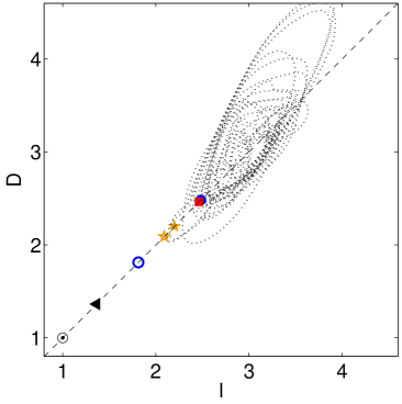
| Re | acc. | freq. | |||||||
|---|---|---|---|---|---|---|---|---|---|
| mean | 0.2828 | 0.087 | 2.926 | ||||||
| 0 | 0.1667 | 1 | 0 | 0 | 2 | ||||
| 0.2091 | 0.1363 | 1.429 | 1 | 1 | 7 | ||||
| 0.3858 | 0.0780 | 3.044 | 8 | 2 | 3 | ||||
| 0.1259 | 0.1382 | 1.318 | 4 | 2 | 2 | ||||
| 0.1681 | 0.1243 | 1.454 | 6 | 3 | 8 | ||||
| 0.2186 | 0.1073 | 2.020 | 11 | 4 | 1 | ||||
| 330 | 0.2751 | 0.0972 | 2.818 | 19 | 6 | ||||
| 0.0935 | 0.1469 | 1.252 | 3 | 1 | 3 | ||||
| 0.1756 | 0.1204 | 3.044 | 15 | 2 | |||||
| 0.1565 | 0.1290 | 1.404 | 5 | 3 | 1 | ||||
| 0.3285 | 0.1080 | 2.373 | 10 | 7 | |||||
| 0.4049 | 0.0803 | 3.432 | 13 | 10 | |||||
| 0.3037 | 0.1159 | 2.071 | 5 | 4 | |||||
| 0.4049 | 0.0813 | 3.361 | 15 | 9 |
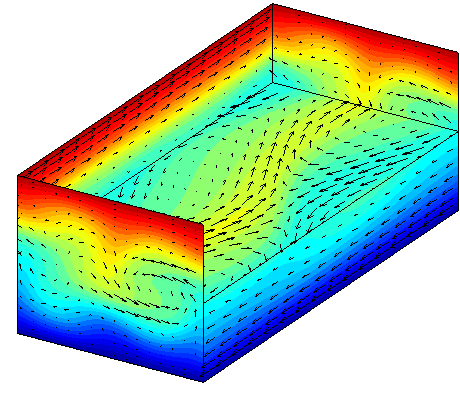
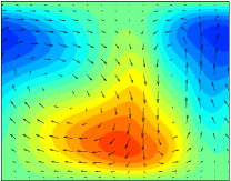
, . The lower-branch solution was found only once in our 28 searches, and its upper-branch partner only by continuation in Reynolds number. We were only able to continue up to . At this value it is highly unstable, with a 19 dimensional unstable manifold, and it is far more dissipative than a typical turbulent trajectory.
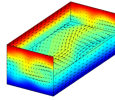
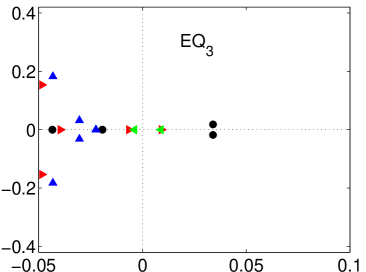
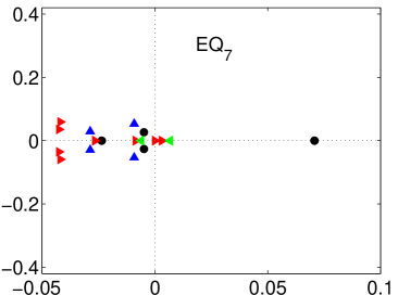
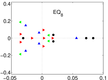
, appear together in a saddle node bifurcation in Re (see § 5). / might be the same as Schmiegel (1999)’s ‘ solutions’. The -average velocity field plots appear very similar, as do the versus Re bifurcation diagrams. We were not able to obtain Schmiegel’s data in order to make a direct comparison. is both the closest state to laminar in terms of disturbance energy and the lowest in terms of drag. It has one strongly unstable real eigenvalue within the -invariant subspace and two weakly unstable eigenvalues with and antisymmetries, respectively. In this regard, the EQ7 unstable manifold might, like the unstable manifold of , form part of the boundary between the laminar basin of attraction and turbulence. and are unique among the equilibria determined here in that they have the order-8 isotropy subgroup (see § 3.2). The action of the quotient group yields 2 copies of each, plotted in figure 3. and are similar in appearance to and , except for the additional symmetry.
is a single lopsided roll-streak pair. It is produced by a pitchfork bifurcation from at as an -antisymmetric eigenfunction goes through marginal stability (the only pitchfork bifurcation we have yet found) and remains close to at . Thus, it has isotropy. Even though is not -isotropic, we found it from a search initiated on a guess that was -isotropic to single precision. Such small asymmetries were enough to draw the Newton-hookstep search algorithm out of the -invariant subspace.
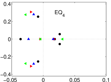
, are produced in a saddle-node bifurcation at as a lower / upper branch pair, and they lie close to the center of mass of the turbulent repeller, see figure 8 (a). The velocity fields have a similar appearance to typical turbulent states for this cell size. However, they are both highly unstable and unlikely to be revisited frequently by a generic turbulent fluid state. Their isotropy subgroup is order 2, so the action of the quotient group yields 8 copies of each, which appear as the 4 overlaid pairs in projections onto the (16) basis set, see figure 1 and figure 3. , were found by continuation of in .
4.2 Traveling waves
The first two traveling-wave solutions reported in the literature were found by Nagata (1997) by continuing equilibrium to a combined Couette / Poiseuille channel flow, and then continuing back to plane Couette flow. The result was a pair of streamwise traveling waves arising from a saddle-node bifurcation. Viswanath (2008) found two traveling waves, ‘D1’ and the same solution ‘D2,’ but at a higher , through an edge-tracking algorithm (Skufca et al. (2006), see also § 4.1). Here we verify Viswanath’s solution and present two new traveling-wave solutions computed as symmetry-breaking bifurcations off equilibrium solutions. We were not able to compare these to Nagata’s traveling waves since the data is not available. The traveling waves are shown as 3D velocity fields in figure 9 and as closed orbits in state space in figure 3. Their kinetic energies and dissipation rates are tabulated in table 1. Each traveling-wave solution has a zero spatial-mean pressure gradient but non-zero mean velocity in the same direction as the wave velocity. It is likely each solution could be continued to zero wave velocity but non-zero spatial-mean pressure gradient.
traveling wave is -isotropic and hence spanwise traveling. At its velocity is very small, , and it has a small but nonzero mean velocity, also in the spanwise direction. This is a curious property: induces bulk transport of fluid without a pressure gradient, and in a direction orthogonal to the motion of the walls. was found as a pitchfork bifurcation from , and thus lies very close to it in state space. It is weakly unstable, with a unstable manifold with two eigenvalues which are extremely close to marginal. In this sense unstable manifold is nearly one-dimensional, and comparable to .
is a streamwise traveling wave found by Viswanath (2008) and called D1 there. It is -isotropic, has a low dissipation rate, and a small but nonzero mean velocity in the streamwise direction. Viswanath provided data for this solution; we verified it with an independent numerical integrator and continued the solution to cell for comparison with the other traveling waves. In this cell is fairly stable, with an eigenspectrum similar to ’s, except with different symmetries.
is an -isotropic streamwise traveling wave with a relatively high wave velocity and a nonzero mean velocity in the streamwise direction. Its dissipation rate and energy norm are close to those of .

5 Continuation under Reynolds number
(a)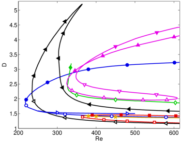 (b)
(b)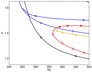
The relations between the equilibrium and traveling-wave solutions can be clarified by tracking their properties under changes in Re and spatial periodicity. Figure 10 shows a bifurcation diagram for equilibria and traveling waves in the cell, with dissipation rate plotted against as the bifurcation parameter. A number of independent solution curves are shown in superposition. This is a 2-dimensional projection from the -dimensional state space, thus, unless noted otherwise, the apparent intersections of the solution curves do not represent bifurcations; rather, each curve is a family of solutions with an upper and lower branch, beginning with a saddle-node bifurcation at a critical Reynolds number.
The first saddle-node bifurcation gives birth to the Nagata lower branch and upper branch equilibria, at . has a single -isotropic unstable eigenvalue (and additional subharmonic instabilities that break the -isotropy of ). Shortly after bifurcation, has an unstable complex eigenvalue pair within the -invariant subspace and two unstable real eigenvalues leading out of that space. As indicated by the gentle slopes of their bifurcation curves, the Nagata (1990) solutions are robust with respect to Reynolds number. The lower branch solution has been continued past and has a single unstable eigenvalue throughout this range (Wang et al., 2007).
and are formed in a saddle-node bifurcation at . The bifurcation curve is unusual in that it increases rapidly from the bifurcation point to a maximum dissipation of at , and then turns rapidly but smoothly back down to much lower dissipation at higher Reynolds numbers. This behavior persists when examined at higher spatial and temporal resolutions.
and were discovered in independent Newton searches and subsequently found by continuation to be lower and upper branches of a saddle-node bifurcation occurring at . has a leading unstable complex eigenvalue pair within the -invariant subspace. Its remaining two unstable eigen-directions are nearly marginal and lead out of this space.
was found by continuing backwards in Re around the bifurcation point at . We were not able to continue past . At this point it has a nearly marginal stable pair of eigenvectors whose isotropy group is , which rules out a bifurcation to traveling waves along these modes. Just beyond the dynamics in this region appears to be roughly periodic, suggesting that undergoes a supercritical Hopf bifurcation here. At , , are born in a saddle node bifurcation, similar in character to the / bifurcation, as are , .
Figure 10(b) shows several symmetry-breaking bifurcations. At , bifurcates from in a subcritical pitchfork as an -symmetric, -antisymmetric eigenfunction of becomes unstable, resulting in a spanwise-moving traveling wave. At , the equilibrium bifurcates off along an -antisymmetric, -symmetric eigenfunction of . Since symmetry fixes phase in both and , this solution bifurcates off as an equilibrium rather than a traveling wave.
Figure 11(a) shows the instability of each equilibrium as a function of Reynolds number. As a measure of instability we use the sum of the real parts of the equilibrium’s unstable eigenvalues, i.e. the local exponential rate of stretching of the equilibrium’s unstable manifold. Several observations can be made. Each lower-branch solution (open symbol) is less unstable than its upper-branch counterpart (closed symbol). Lower branch solutions tend towards lesser instability as Reynolds number increases, upper branch solutions become more unstable. Since lower/upper branches of a given solution are defined by lower/higher dissipation rates, this implies that lower instability and lower dissipation go hand in hand. However this relation does not generally hold between different solution branches: has lower dissipation than (figure 10(a)) but is more unstable (Figure 11(a)). Several of the lower-branch solutions have very slowly decreasing instability over the range of Reynolds numbers shown; for these, the number of unstable eigenvalues is constant or slowly decreasing as well. has three unstable eigenvalues shortly after bifurcation and just one for , has six after bifurcation and three for , has four from bifurcation onwards, , and has eight from bifurcation onwards, . The upper limits of these ranges are merely the endpoints of our calculations. Clever & Busse (1997) show that at certain wavenumbers, is stable for a small range of Reynolds numbers just after bifurcation. We did not look for or find regions of stability for any of the new solutions, though we expect such regions exist for carefully tuned parameters. For example, a stable periodic orbit has been found in the related Kuramoto-Sivashinsky system (Lan & Cvitanović, 2008). For the upper branch solutions generally both the numbers of unstable eigenvalues as well as their sums increase with Re. Lastly, it should be remembered that it is not at all clear how much the instability of an equilibrium has to do with the Lyapunov exponents of the turbulent flow - that depends on how close and how frequently a typical trajectory visits the neighborhood of a given equilibrium.
6 Continuation under spanwise wavenumber
(a) 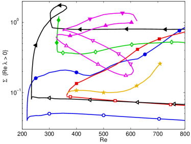 (b)
(b) 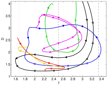
In this section we examine changes in solutions under variation in spanwise periodicity. Figure 11(b) shows the dissipation of the solutions as a function of spanwise wavenumber . Only a few of the intersections in this plot indicate bifurcations; the rest are artifacts of the projection onto the plane. The true bifurcations are branching off from near ; from near ; and from near . Continuation in also shows that the , and , solution curves, which appear to be independent in figure 10, are connected by a saddle-node bifurcation between and near .
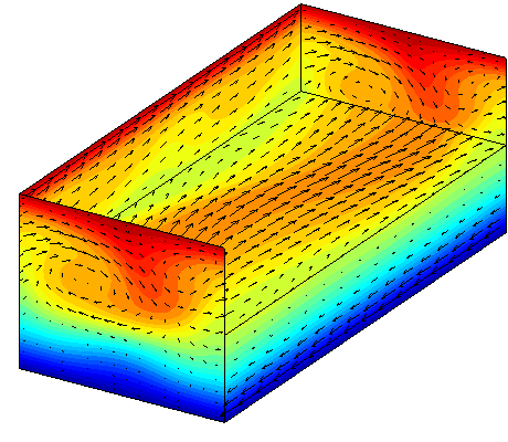
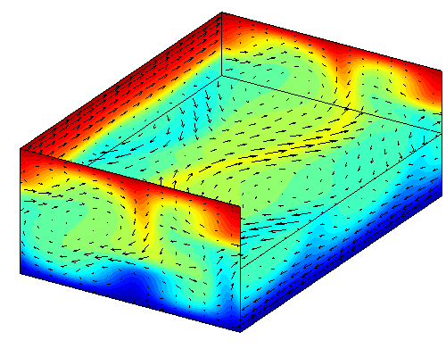
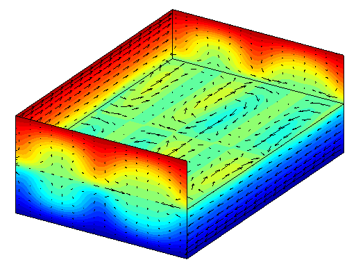
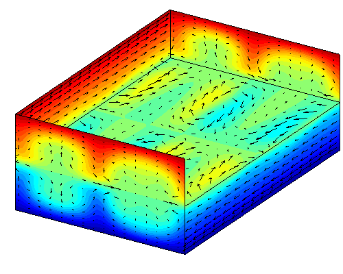
In addition to these bifurcations, we are interested in connecting the solutions for discussed in § 4, to the wider cell of Hamilton et al. (1995), which empirically exhibits turbulence for long time scales at . Of the equilibria discussed above, only , , , and could be continued at from of down to the fundamental wavenumber of . appears in a saddle-node bifurcation just below . The other equilibria terminate in saddle-node bifurcations above or at bifurcations from other solution curves. However, the and solutions can be continued upwards in to the first harmonic of (). These solutions then appear in as as spanwise “doubled” states and . Figure 12 shows 3D velocity fields for equilibria in : , , , and and the spanwise doubled and . The upper branch of not shown, is very similar to . The properties of these solutions are listed in table 3.
The low dissipation values of the equilibria in figure 8 (b) suggest that they are not involved in turbulent dynamics, except perhaps as gatekeepers to the laminar equilibrium. We suspect that the equilibria as yet undiscovered, or the already known periodic orbit solutions (Gibson & Cvitanović, 2009) do play a key role in organizing turbulent dynamics. However, unlike the cell, we were not able to find any equilibria for cell from initial guesses sampled from turbulent trajectories within the -invariant subspace. This is curious, contrasted to our success in finding equilibria from such guesses in , and it suggests that the aspect ratios of the cell are the most incommensurate (fit the intrinsic widths of rolls least well) compared to the roll and streak scales of spanwise-infinite domains, which are apparent (approximately) in the simulation of figure 2. The stability calculations by Clever & Busse (1997) indicate that the Nagata solutions prefer a 2:1 streamwise to spanwise aspect ratio. Hence a study of changes in solutions under variation in both streamwise and spanwise periodicities might shed further light on the physical nature of these solutions.
| acc. | |||||||
|---|---|---|---|---|---|---|---|
| mean | 0.40 | 0.15 | 3.0 | ||||
| 0 | 0.1667 | 1 | 0 | 0 | |||
| 0.2458 | 0.1112 | 1.8122 | 5 | 3 | |||
| 0.3202 | 0.0905 | 2.4842 | 6 | 2 | |||
| 0.2853 | 0.0992 | 2.4625 | 40 | 13 | |||
| 0.1261 | 0.1433 | 1.3630 | 6 | 2 | |||
| 0.1969 | 0.1186 | 1.7967 | 19 | 1 | |||
| 0.3159 | 0.1175 | 2.0900 | 11 | 0 | |||
| (upper) | 0.3276 | 0.1119 | 2.2000 | 16 | 5 |
7 Conclusion and perspectives
As a turbulent flow evolves, every so often we catch a glimpse of a familiar pattern. For any finite spatial resolution, the flow approximately follows for a finite time a pattern belonging to a finite alphabet of admissible fluid states, represented here by a set of equilibrium and traveling wave solutions of Navier-Stokes. These are not the ‘modes’ of the fluid; they do not provide a decomposition of the flow into a sum of components at different wavelengths, or a projection basis for low-dimensional modeling. Each solution spans the whole range of physical scales of the turbulent fluid, from the outer wall-to-wall scale, down to the viscous dissipation scale. Numerical computations require sufficient resolution to cover all of these scales, so no global dimension reduction is likely. The role of invariant solutions of Navier-Stokes is, instead, to partition the -dimensional state space into a finite set of neighborhoods visited by a typical long-time turbulent fluid state.
Motivated by the recent observations of recurrent coherent states in experiments and numerical studies, we undertook here an exploration of the hierarchy of all known equilibria and traveling waves of fully-resolved plane Couette flow in order to describe the spatio-temporally chaotic dynamics of transitionally turbulent fluid flows. Turbulent plane Couette dynamics visualized in state space appears pieced together from close visitations to coherent states connected by transient interludes, as can be seen in Gibson (2008b) animations of figure 2. The fluid states explored by the small aspect-ratio equilibria and their unstable manifolds studied in this paper are strikingly similar to states observed in larger aspect-ratio simulations, such as figure 2.
For plane Couette flow equilibria, traveling waves and periodic solutions embody a vision of turbulence as a repertoire of recurrent spatio-temporal patterns explored by turbulent dynamics. The new equilibria and traveling waves that we present here form the backbone of this repertoire. Currently, a taxonomy of these myriad states eludes us, but emboldened by successes in applying periodic orbit theory to the simpler, warm-up Kuramoto-Sivashinsky problem (Christiansen et al., 1997; Lan & Cvitanović, 2008; Cvitanović et al., 2009), we are optimistic. Given a set of equilibria, the next step is to understand how the dynamics interconnects the neighborhoods of the invariant solutions discovered so far; a task that we address in Halcrow et al. (2009) which discusses their heteroclinic connections, and Gibson & Cvitanović (2009) which discusses their periodic orbit solutions.
The reader might rightfully wonder what the small-aspect periodic cells studied here have to do with physical plane Couette flow and wall-bounded shear flows in general, with large aspect ratios and physical spanwise-streamwise boundary conditions. Indeed, the outstanding issue that must be addressed in future work is the small-aspect cell periodicities imposed for computational efficiency. So far, most computations of invariant solutions have focused on spanwise-streamwise (axial-streamwise in case of the pipe flow) periodic cells barely large enough to allow for sustained turbulence. Such small cells introduce dynamical artifacts such as lack of structural stability and cell-size dependence of the sustained turbulence states. However, every solution that we find is also a solution of the infinite aspect-ratio problem, i.e., a solution whose finite cell tiles the infinite plane Couette flow. As we saw in § 6, under a continuous variation of spanwise length such solutions come in continuous families whose fundamental wavelengths reflect the roll and streak instability scales observed in large-aspect systems such as figure 2. Here we can draw the inspiration from pattern-formation theory, where the most unstable wavelengths from a continuum of unstable solutions set the scales observed in simulations.
Acknowledgements.
We would like to acknowledge F. Waleffe for providing his equilibrium solution data and for his very generous guidance through the course of this research. We greatly appreciate discussions with D. Viswanath, his guidance in numerical algorithms, and for providing his traveling wave data. We are indebted to G. Kawahara, L.S. Tuckerman, B. Eckhardt, D. Barkley, and J. Elton for inspiring discussions. P.C., J.F.G. and J.H. thank G. Robinson, Jr. for support. J.F.G. was partly supported by NSF grant DMS-0807574. J.H. thanks R. Mainieri and T. Brown, Institute for Physical Sciences, for partial support. Special thanks to the Georgia Tech Student Union which generously funded our access to the Georgia Tech Public Access Cluster Environment (GT-PACE), essential to the computationally demanding Navier-Stokes calculations. [Note added in proof: since submission of this article it has come to our attention that Itano & Generalis (2009) have independently determined the , equilibria.]References
- Canuto et al. (1988) Canuto, C., Hussaini, M. Y., Quarteroni, A. & Zang, T. A. 1988 Spectral Methods in Fluid Dynamics. Springer-Verlag.
- Cherhabili & Ehrenstein (1997) Cherhabili, A. & Ehrenstein, U. 1997 Finite-amplitude equilibrium states in plane Couette flow. J. Fluid Mech. 342, 159–177.
- Christiansen et al. (1997) Christiansen, F., Cvitanović, P. & Putkaradze, V. 1997 Spatio-temporal chaos in terms of unstable recurrent patterns. Nonlinearity 10, 55–70.
- Clever & Busse (1992) Clever, R. M. & Busse, F. H. 1992 Three-dimensional convection in a horizontal layer subjected to constant shear. J. Fluid Mech. 234, 511–527.
- Clever & Busse (1997) Clever, R. M. & Busse, F. H. 1997 Tertiary and quaternary solutions for plane Couette flow. J. Fluid Mech. 344, 137–153.
- Cvitanović et al. (2009) Cvitanović, P., Davidchack, R. L. & Siminos, E. 2009 On state space geometry of the kuramoto-sivashinsky flow in a periodic domain. arXiv:0709.2944, SIAM J. Appl. Dynam. Systems, to appear.
- Duguet et al. (2008) Duguet, Y., Pringle, C. C. T. & Kerswell, R. R. 2008 Relative periodic orbits in transitional pipe flow. arXiv:0807.2580.
- Ehrenstein et al. (2008) Ehrenstein, U., Nagata, M. & Rincon, F. 2008 Two-dimensional nonlinear plane Poiseuille-Couette flow homotopy revisited. Phys. Fluids 20, 064103–1–4.
- Faisst & Eckhardt (2003) Faisst, H. & Eckhardt, B. 2003 Traveling waves in pipe flow. Phys. Rev. Lett. 91, 224502.
- Frisch (1996) Frisch, U. 1996 Turbulence. Cambridge, UK: Cambridge University Press.
- Gibson (2008a) Gibson, J. F. 2008a Channelflow: a spectral Navier-Stokes simulator in C++. Tech. Rep.. Georgia Inst. of Technology, Channelflow.org.
- Gibson (2008b) Gibson, J. F. 2008b Movies of plane Couette. Tech. Rep.. Georgia Institute of Technology, ChaosBook.org/tutorials.
- Gibson & Cvitanović (2009) Gibson, J. F. & Cvitanović, P. 2009 Periodic orbits of plane Couette flow. In preparation.
- Gibson et al. (2008) Gibson, J. F., Halcrow, J. & Cvitanović, P. 2008 Visualizing the geometry of state-space in plane Couette flow. J. Fluid Mech. 611, 107–130, arXiv:0705.3957.
- Gilmore & Letellier (2007) Gilmore, R. & Letellier, C. 2007 The Symmetry of Chaos. Oxford: Oxford Univ. Press.
- Golubitsky & Stewart (2002) Golubitsky, M. & Stewart, I. 2002 The symmetry perspective. Boston: Birkhäuser.
- Halcrow (2008) Halcrow, J. 2008 Geometry of turbulence: An exploration of the state-space of plane Couette flow. PhD thesis, School of Physics, Georgia Inst. of Technology, Atlanta, ChaosBook.org/projects/theses.html.
- Halcrow et al. (2009) Halcrow, J., Gibson, J. F., Cvitanović, P. & Viswanath, D. 2009 Heteroclinic connections in plane Couette flow. J. Fluid Mech. 621, 365–376, arXiv:0808.1865.
- Hamilton et al. (1995) Hamilton, J. M., Kim, J. & Waleffe, F. 1995 Regeneration mechanisms of near-wall turbulence structures. J. Fluid Mech. 287, 317–348.
- Harter (1993) Harter, W. G. 1993 Principles of Symmetry, Dynamics, and Spectroscopy. New York: Wiley.
- Hof et al. (2004) Hof, B., van Doorne, C. W. H., Westerweel, J., Nieuwstadt, F. T. M., Faisst, H., Eckhardt, B., Wedin, H., Kerswell, R. R. & Waleffe, F. 2004 Experimental observation of nonlinear traveling waves in turbulent pipe flow. Science 305 (5690), 1594–1598, www.sciencemag.org/cgi/reprint/305/5690/1594.pdf.
- Hoyle (2006) Hoyle, R. 2006 Pattern Formation: An Introduction to Methods. Cambridge: Cambridge Univ. Press.
- Itano & Generalis (2009) Itano, T. & Generalis, S. C. 2009 Hairpin vortex solution in planar Couette flow: A tapestry of knotted vortices. Phys. Rev. Lett. 102, 114501.
- Itano & Toh (2001) Itano, T. & Toh, S. 2001 The dynamics of bursting process in wall turbulence. J. Phys. Soc. Japan 70, 701–714.
- J.E. Dennis, Jr., & Schnabel (1996) J.E. Dennis, Jr., & Schnabel, R. B. 1996 Numerical Methods for Unconstrained Optimization and Nonlinear Equations. Philadelphia: SIAM.
- Jiménez et al. (2005) Jiménez, J., Kawahara, G., Simens, M. P., Nagata, M. & Shiba, M. 2005 Characterization of near-wall turbulence in terms of equilibrium and bursting solutions. Phys. Fluids 17, 015105.
- Kim et al. (1971) Kim, H., Kline, S. & Reynolds, W. 1971 The production of turbulence near a smooth wall in a turbulent boundary layer. J. Fluid Mech. 50, 133–160.
- Kleiser & Schumann (1980) Kleiser, L. & Schumann, U. 1980 Treatment of incompressibility and boundary conditions in 3-D numerical spectral simulations of plane channel flows. In Proc. 3rd GAMM Conf. Numerical Methods in Fluid Mechanics (ed. E. Hirschel), pp. 165–173. GAMM, Viewweg, Braunschweig.
- Lan & Cvitanović (2008) Lan, Y. & Cvitanović, P. 2008 Unstable recurrent patterns in Kuramoto-Sivashinsky dynamics. Phys. Rev. E 78, 026208, arXiv.org:0804.2474.
- Marsden & Ratiu (1999) Marsden, J. E. & Ratiu, T. S. 1999 Introduction to Mechanics and Symmetry. New York, NY: Springer-Verlag.
- Nagata (1990) Nagata, M. 1990 Three-dimensional finite-amplitude solutions in plane Couette flow: bifurcation from infinity. J. Fluid Mech. 217, 519–527.
- Nagata (1997) Nagata, M. 1997 Three-dimensional traveling-wave solutions in plane Couette flow. Phys. Rev. E 55, 2023–2025.
- Peyret (2002) Peyret, R. 2002 Spectral Methods for Incompressible Flows. Springer-Verlag.
- Pringle & Kerswell (2007) Pringle, C. T. & Kerswell, R. R. 2007 Asymmetric, helical, and mirror-symmetric traveling waves in pipe flow. Phys. Rev. Lett. 99, 074502.
- Rincon (2007) Rincon, F. 2007 On the existence of two-dimensional nonlinear steady states in plane Couette flow. Phys. Fluids 19, 4105–+, arXiv:0706.1165.
- Schmiegel (1999) Schmiegel, A. 1999 Transition to turbulence in linearly stable shear flows. PhD thesis, Philipps-Universität Marburg, available on archiv.ub.uni-marburg.de/diss/z2000/0062.
- Schneider et al. (2008) Schneider, T., Gibson, J., Lagha, M., Lillo, F. D. & Eckhardt, B. 2008 Laminar-turbulent boundary in plane Couette flow. Phys. Rev. E. 78, 037301, arXiv:0805.1015.
- Skufca et al. (2006) Skufca, J. D., Yorke, J. A. & Eckhardt, B. 2006 Edge of chaos in a parallel shear flow. Phys. Rev. Lett. 96 (17), 174101.
- Tuckerman & Barkley (2002) Tuckerman, L. S. & Barkley, D. 2002 Symmetry breaking and turbulence in perturbed plane Couette flow. Theoretical and Computational Fluid Dynamics 16, 91–97, arXiv:physics/0312051.
- Viswanath (2007) Viswanath, D. 2007 Recurrent motions within plane Couette turbulence. J. Fluid Mech. 580, 339–358, arXiv:physics/0604062.
- Viswanath (2008) Viswanath, D. 2008 The dynamics of transition to turbulence in plane Couette flow. In Mathematics and Computation, a Contemporary View. The Abel Symposium 2006, Abel Symposia, vol. 3. Berlin: Springer-Verlag, arXiv:physics/0701337.
- Waleffe (1990) Waleffe, F. 1990 Proposal for a self-sustaining mechanism in shear flows. Center for Turbulence Research, Stanford University/NASA Ames, unpublished preprint (1990).
- Waleffe (1995) Waleffe, F. 1995 Hydrodynamic stability and turbulence: beyond transients to a self-sustaining process. Stud. Applied Math. 95, 319–343.
- Waleffe (1997) Waleffe, F. 1997 On a self-sustaining process in shear flows. Phys. Fluids 9, 883–900.
- Waleffe (1998) Waleffe, F. 1998 Three-dimensional coherent states in plane shear flows. Phys. Rev. Lett. 81, 4140–4143.
- Waleffe (2001) Waleffe, F. 2001 Exact coherent structures in channel flow. J. Fluid Mech. 435, 93–102.
- Waleffe (2002) Waleffe, F. 2002 Exact coherent structures and their instabilities: Toward a dynamical-system theory of shear turbulence. In Proceedings of the International Symposium on “Dynamics and Statistics of Coherent Structures in Turbulence: Roles of Elementary Vortices” (ed. S. Kida), pp. 115–128. National Center of Sciences, Tokyo, Japan.
- Waleffe (2003) Waleffe, F. 2003 Homotopy of exact coherent structures in plane shear flows. Phys. Fluids 15, 1517–1543.
- Wang et al. (2007) Wang, J., Gibson, J. F. & Waleffe, F. 2007 Lower branch coherent states in shear flows: transition and control. Phys. Rev. Lett. 98 (20).
- Wedin & Kerswell (2004) Wedin, H. & Kerswell, R. R. 2004 Exact coherent structures in pipe flow: travelling wave solutions. J. Fluid Mech. 508, 333–371.