Debye Sources and the Numerical Solution
of the Time Harmonic Maxwell Equations

Abstract

In this paper, we develop a new representation for outgoing solutions to the time harmonic Maxwell equations in unbounded domains in $\mathbb{R}^{3}.$ This representation leads to a Fredholm integral equation of the second kind for solving the problem of scattering from a perfect conductor, which does not suffer from spurious resonances or low frequency breakdown, although it requires the inversion of the scalar surface Laplacian on the domain boundary. In the course of our analysis, we give a new proof of the existence of non-trivial families of time harmonic solutions with vanishing normal components that arise when the boundary of the domain is not simply connected. We refer to these as $k$-Neumann fields, since they generalize, to non-zero wave numbers, the classical harmonic Neumann fields. The existence of $k$-harmonic fields was established earlier by Kress.

Introduction

Electromagnetic wave propagation in a uniform, nonconducting, isotropic medium in $\mathbb{R}^{3}$ is described by the Maxwell equations

$$\nabla\times{\cal E}(\boldsymbol{x},t)=-\mu\frac{\partial{\cal H}}{\partial t}\,,\quad\nabla\times{\cal H}(\boldsymbol{x},t)=\epsilon\frac{\partial{\cal E}}{\partial t}\,,$$ (1)

$$\nabla\cdot{\cal E}(\boldsymbol{x},t)=0\,,\quad\nabla\cdot{\cal H}(\boldsymbol{x},t)=0\,,$$

where ${\cal E}$ and ${\cal H}$ denote the electric and magnetic fields, respectively and $\epsilon,\mu$ are the electrical permittivity and magnetic permeability of the medium. We will restrict our attention to the time-harmonic case and write

$${\cal E}(\boldsymbol{x},t)=\operatorname{Re}\left\{\frac{\boldsymbol{E}^{\operatorname{tot}}(\boldsymbol{x})}{\sqrt{\epsilon}}e^{-i\omega t}\right\}\quad{\rm and}\quad{\cal H}(\boldsymbol{x},t)=\operatorname{Re}\left\{\frac{\boldsymbol{H}^{\operatorname{tot}}(\boldsymbol{x})}{\sqrt{\mu}}e^{-i\omega t}\right\}\,.$$ (2)

The superscript is used to emphasize that $\boldsymbol{E}^{\operatorname{tot}}$ and $\boldsymbol{H}^{\operatorname{tot}}$ define the total electric and magnetic fields, respectively. In electromagnetic scattering, they are generally written as a sum

$$\boldsymbol{E}^{\operatorname{tot}}(\boldsymbol{x})=\boldsymbol{E}^{\operatorname{in}}(\boldsymbol{x})+\boldsymbol{E}(\boldsymbol{x}),\qquad\boldsymbol{H}^{\operatorname{tot}}(\boldsymbol{x})=\boldsymbol{H}^{\operatorname{in}}(\boldsymbol{x})+\boldsymbol{H}(\boldsymbol{x}),$$ (3)

where $\{\boldsymbol{E}^{\operatorname{in}},\boldsymbol{H}^{\operatorname{in}}\}$ describe a known incident field and $\{\boldsymbol{E},\boldsymbol{H}\}$ denote the scattered field of interest. With the scaling in (2), the Maxwell equations take the simpler form

$$\nabla\times\boldsymbol{H}^{\operatorname{tot}} = -ik\boldsymbol{E}^{\operatorname{tot}}$$ (4)

$$\nabla\times\boldsymbol{E}^{\operatorname{tot}} = ik\boldsymbol{H}^{\operatorname{tot}}\,.$$

We are particularly interested in the problem of scattering from a perfect conductor in an exterior region, which we denote by $\Omega$. For a perfect conductor [13, 22], the conditions to be enforced on $\Gamma$, the boundary of $\Omega$, are

$$\boldsymbol{n}\times\boldsymbol{E}^{\operatorname{tot}}=0,\qquad\boldsymbol{n}\cdot\boldsymbol{H}^{\operatorname{tot}}=0.$$ (5)

The scattered field is assumed to satisfy the Silver-Müller radiation condition:

$$\lim_{r\rightarrow\infty}\left(\boldsymbol{H}\times\frac{\boldsymbol{r}}{r}-\boldsymbol{E}\right)=o\left(\frac{1}{r}\right).$$ (6)

This problem has been studied rather intensively for many decades, and we do not seek to review the literature here, except to observe that there are two distinct approaches in widespread use. When the scatterer is a sphere, a simple and elegant theory exists due to Lorenz, Debye and Mie [6, 10, 16, 19]. It is based on two scalar potentials (generally called Debye potentials), and the mathematical machinery of vector spherical harmonics. In particular, one represents $\boldsymbol{E}$, $\boldsymbol{H}$ as

$$\boldsymbol{E} = \nabla\times\nabla\times(\boldsymbol{r}v)\,+\,ik\nabla\times(\boldsymbol{r}u)$$

$$\boldsymbol{H} = \nabla\times\nabla\times(\boldsymbol{r}u)-ik\nabla\times(\boldsymbol{r}v)$$ (7)

where the Debye potentials $u,v$ satisfy the scalar Helmholtz equation

$$\Delta u+k^{2}u=0,\ \Delta v+k^{2}v=0\ ,$$

with Helmholtz parameter (wave number) $k^{2}=\omega^{2}\epsilon\mu$. Salient features of this approach are (a) that the boundary value problem

$$\boldsymbol{n}\times\boldsymbol{E} = -\boldsymbol{n}\times\boldsymbol{E}^{\operatorname{in}}$$ (8)

$$\boldsymbol{n}\cdot\boldsymbol{H} = -\boldsymbol{n}\cdot\boldsymbol{H}^{\operatorname{in}}$$ (9)

is uniquely solvable for any $k$ with non-negative imaginary part and (b) that, as $k\rightarrow 0$ ($\omega\rightarrow 0$), the electric and magnetic fields uncouple gracefully. In the static limit, $\boldsymbol{E}$ is due to the scalar potential $v$ alone, which is, in turn, determined by the boundary data $-\boldsymbol{n}\times\boldsymbol{E}^{\operatorname{in}}$. Likewise, $\boldsymbol{H}$ is due to the scalar potential $u$ alone, which is determined by the boundary data $-\boldsymbol{n}\cdot\boldsymbol{H}^{\operatorname{in}}$.

For regions of arbitrary shape, on the other hand, integral formulations of the Maxwell equations are generally based on the classical vector and scalar potentials (in the Lorenz gauge):

$$\boldsymbol{E} = ik\boldsymbol{A}-\nabla\phi$$ (10)

$$\boldsymbol{H} = \nabla\times\boldsymbol{A}$$ (11)

where

$$\boldsymbol{A}(\boldsymbol{x})=\int_{\Gamma}g_{k}(\boldsymbol{x}-\boldsymbol{y})\boldsymbol{J}(\boldsymbol{y})dA_{\boldsymbol{y}}$$

$$\phi(\boldsymbol{x})=\frac{1}{ik}\int_{\Gamma}g_{k}(\boldsymbol{x}-\boldsymbol{y})(\nabla_{\Gamma}\cdot\boldsymbol{J})(\boldsymbol{y})dA_{\boldsymbol{y}}$$

with

$$g_{k}(\boldsymbol{x})=\frac{e^{ik|\boldsymbol{x}|}}{4\pi|\boldsymbol{x}|}\,.$$

Here, $\boldsymbol{J}$ is a surface current (a tangential vector field) and $\nabla_{\Gamma}\cdot\boldsymbol{J}$ denotes its surface divergence.

Maue [17] proposed the electric field integral equation (EFIE) for the unknown current $\boldsymbol{J}$ by enforcing the condition (8) using the representation (10). Because of the $\nabla\phi$ term, however, the result is a hypersingular equation. Maue also proposed the magnetic field integral equation (MFIE), based on (11). The boundary condition for $\boldsymbol{H}$ can be derived from the Maxwell equations and an appropriate limiting process on the surface of a perfect conductor [13, 22]:

$$\boldsymbol{J}=\boldsymbol{n}\times\boldsymbol{H}^{\operatorname{in}}+\boldsymbol{n}\times\boldsymbol{H}\,,$$ (12)

where $\boldsymbol{n}$ points into $\Omega$. Enforcing this condition for the unknown current $\boldsymbol{J}$ yields the MFIE, a second kind Fredholm equation. Unfortunately, both the MFIE and the EFIE have spurious resonances; that is, there exists a countable set of frequencies $\{k_{j}\}\subset\mathbb{R}$ for which the integral equations are not invertible. As the $\{k_{j}\}$ are the eigenvalues of a self adjoint, elliptic boundary value problem on the bounded complement of $\Omega,$ they are often referred to as interior resonances. Below the smallest such $k_{j}$, the MFIE is well-conditioned. Spurious resonances, however, are only one difficulty. A second problem stems from the representation of the electric field itself. Unlike the Debye representation, the electric field does not uncouple naturally from the magnetic field as $k\rightarrow 0$. Note that in (10), $\boldsymbol{E}$ involves one term of order $k$ and one term of order $k^{-1}$. This results in what is referred to as “low-frequency breakdown” [36]. While low frequency breakdown is a more transparent problem in the context of the EFIE, the MFIE is not immune [35]. Knowing the current $\boldsymbol{J}$ is sufficient for computing $\boldsymbol{H}$, but not the electric field. The normal component of $\boldsymbol{E}$, for example, is determined by the electric charge:

$$\boldsymbol{n}\cdot\boldsymbol{E}=\rho=\frac{\nabla_{\Gamma}\cdot\boldsymbol{J}}{ik}\,.$$ (13)

As $k\rightarrow 0$, accuracy degrades dramatically - a phenomenon called “catastrophic cancellation” in numerical analysis.

This state of affairs is both odd and unsatisfactory. For the exterior of a sphere, there is a simple, clean representation of the solution based on two scalar unknowns that results in a diagonal linear system. It has no spurious resonances and, at zero frequency, decouples naturally (with no loss of precision) into magnetostatic and electrostatic problems. The standard integral equation approaches available for general geometries do not reduce to a Debye-like formalism when restricted to a sphere. Instead, a sequence of modifications have been introduced to address the three problems discussed above: the existence of spurious resonances, the lack of a second kind integral equation valid for all frequencies, and the loss of accuracy due to low-frequency breakdown.

An important step in addressing the first problem was the introduction in the 1970’s of the combined field integral equation (CFIE) [20, 25]. The CFIE avoids spurious resonances by taking a complex linear combination of the EFIE and the MFIE, both of which involve the surface current as the unknown. It is not a Fredholm equation of the second kind, however, and still suffers from low frequency breakdown. One alternative approach, due to Yaghjian [33], involves augmenting the MFIE with the condition (9) or the EFIE with the condition (13). He showed that (for geometries other than the sphere) the augmented equations yield unique solutions at all frequencies. Of the many formulations that have been introduced to overcome spurious resonances, variants of the CFIE have emerged as the most frequently used in practice.

For the second problem, the principal issue is that of overcoming the hypersingular behavior of the CFIE. One solution is to introduce electric charge $\rho$ as an additional variable [27]. In this approach, one defines the scalar potential $\phi$ by

$$\phi(\boldsymbol{x})=\int_{\Gamma}g_{k}(\boldsymbol{x}-\boldsymbol{y})\rho(\boldsymbol{y})dA_{\boldsymbol{y}}$$ (14)

and imposes the continuity condition

$$\nabla\cdot\boldsymbol{J}=ik\rho.$$ (15)

While the hypersingular term is avoided, one must solve a Fredholm integral equation subject to a differential-algebraic constraint (15). During the last several years, several promising approaches have been developed based on the construction of preconditioners. Christiansen and Nédélec [7] designed effective strategies for the EFIE based on Calderon formulas and the Helmholtz decomposition. Adams and Contopanagos et al. [1, 9] made use of the fact that the EFIE operator serves as its own preconditioner; more precisely, the composition of the hypersingular operator with itself equals the sum of the identity operator and a compact operator. A combined field integral equation using this preconditioned EFIE is both resonance-free and takes the form of a Fredholm equation of the second kind. Preconditioners have also been designed through the use of high frequency asymptotics [2]. Unfortunately, the implementation of these schemes can be rather involved on arbitrary surfaces and, like the MFIE, they still suffers from a form of low-frequency breakdown in the evaluation of $\boldsymbol{E}$ once the integral equation has been solved.

Finally, the third problem - namely the low-frequency breakdown of the integral equations - has generally been handled through the use of specialized basis functions in the discretization of the current, such as the “loop and tree” method of [31, 32]. This is a kind of discrete surface Helmholtz decomposition of $\boldsymbol{J}$. As the frequency goes to zero, the irrotational and solenoidal discretization elements become uncoupled, avoiding the scaling problem that causes loss of precision.

We have chosen to investigate a rather different line of thought, motivated largely by the desire to extend the Debye potentials to surfaces of arbitrary shape. In essence, the Lorenz-Debye-Mie approach is based on expanding the potentials $u,v$ from (7) as

$$v(r,\theta,\phi) = \sum_{n,m}a_{n,m}h^{(1)}_{n}(kr)Y_{n}^{m}(\theta,\phi)$$

$$u(r,\theta,\phi) = \sum_{n,m}b_{n,m}h^{(1)}_{n}(kr)Y_{n}^{m}(\theta,\phi)$$

where $h^{(1)}_{n}(x)$ is the spherical Hankel function of order $n$, and $Y_{n}^{m}(\theta,\phi)$ is the usual spherical harmonic of order $n$ and degree $m$. This separation of variables approach is clearly not suitable in general. From a mathematical viewpoint, it works because of the close connection between the Laplacian in $\mathbb{R}^{3}$ and the surface Laplace-Beltrami operator on the sphere. It is also worth noting that the Lorenz-Debye-Mie approach is not equivalent to a Fredholm equation of the second kind. It is invertible, resonance free and behaves properly at low frequencies, but it is hypersingular. Numerical difficulties are avoided simply because it is in diagonal form.

The features of the Debye potentials that we wish to retain are their symmetry and the fact that, at zero frequency, the system uncouples into separate electrostatic and magnetostatic problems. For symmetry, we begin by using both potentials ($\boldsymbol{A},\phi$) and “antipotentials” $(\boldsymbol{A}_{m},\phi_{m})$ as a formal representation of the electromagnetic fields [22]:

$$\boldsymbol{E} = ik\boldsymbol{A}-\nabla\phi-\nabla\times\boldsymbol{A}_{m}$$ (16)

$$\boldsymbol{H} = \nabla\times\boldsymbol{A}+ik\boldsymbol{A}_{m}-\nabla\phi_{m}$$ (17)

where

$$\boldsymbol{A}(\boldsymbol{x}) = \int_{\Gamma}g_{k}(\boldsymbol{x}-\boldsymbol{y})\boldsymbol{j}(\boldsymbol{y})dA_{\boldsymbol{y}}\,,$$

$$\phi(\boldsymbol{x}) = \int_{\Gamma}g_{k}(\boldsymbol{x}-\boldsymbol{y})r(\boldsymbol{y})dA_{\boldsymbol{y}}\,,$$ (18)

$$\boldsymbol{A}_{m}(\boldsymbol{x}) = \int_{\Gamma}g_{k}(\boldsymbol{x}-\boldsymbol{y})\boldsymbol{m}(\boldsymbol{y})dA_{\boldsymbol{y}}\,,$$

$$\phi_{m}(\boldsymbol{x}) = \int_{\Gamma}g_{k}(\boldsymbol{x}-\boldsymbol{y})q(\boldsymbol{y})dA_{\boldsymbol{y}}\,,$$

together with the continuity conditions

$$\nabla_{\Gamma}\cdot\boldsymbol{j}=ikr\ ,\quad\nabla_{\Gamma}\cdot\boldsymbol{m}=ikq.$$ (19)

Such a symmetric formulation is commonly used for scattering from a dielectric. For the perfect conductor, it underlies the combined source integral equation method (CSIE) [18], where $\boldsymbol{j}$ and $\boldsymbol{m}$ are both assumed to be derived from a ”parent” current distribution $\widetilde{\boldsymbol{j}}$:

$$\boldsymbol{j}=\alpha\widetilde{\boldsymbol{j}},\quad\boldsymbol{m}=(1-\alpha)\boldsymbol{n}\times\widetilde{\boldsymbol{j}}\,$$

for some parameter $\alpha$. More precisely, the CSIE is derived using (16) with the vector unknown $\widetilde{\boldsymbol{j}}$ and enforcing the condition (8). Like the CFIE, it is a resonance-free but hypersingular equation. It is important to recognize that, in this construction, the unknowns $\boldsymbol{j},r,\boldsymbol{m},q$ are no longer physical quantities. $\boldsymbol{j}$ and $r$ correspond to fictitious electric current and electric charge, while $\boldsymbol{m}$ and $q$ correspond to fictitious magnetic current and magnetic charge. Perfect conductors do not support the latter. If the “physical” current supported on the surface $\Gamma$ is desired, it must be computed in a second step. From (12), for example, we have $\boldsymbol{J}=\boldsymbol{n}\times(\boldsymbol{H}^{\operatorname{in}}+\boldsymbol{H})$. This will not be the unknown $\boldsymbol{j}$.

The second and critical feature of our method is that we will use $r$ and $q$ as unknowns and construct $\boldsymbol{j}$ and $\boldsymbol{m}$ from them in such a way that the continuity conditions (19) are automatically satisfied. In particular, for simply connected domains, we will let

$$\boldsymbol{j} =\nabla_{\Gamma}\Psi+\boldsymbol{n}\times\nabla_{\Gamma}\Psi_{m}$$ (20)

$$\boldsymbol{m} =\boldsymbol{n}\times\boldsymbol{j}$$

where

$$\Delta_{\Gamma}\Psi\equiv\nabla_{\Gamma}^{2}\Psi = ikr$$ (21)

$$\Delta_{\Gamma}\Psi\equiv\nabla_{\Gamma}^{2}\Psi_{m} = -ikq\,.$$

We wil refer to $\Delta_{\Gamma}$ as the surface Laplacian or Laplace-Beltrami operator. (In geometry, this name is usually applied to $-\Delta_{\Gamma}$ so that it is a non-negative operator, but we will use the the convention above consistently.) In any case, we will obtain the Helmholtz decomposition of the currents on the surface by construction. This avoids the obvious cause of low-frequency breakdown, since we never compute the $O(1)$ quantities $r,q$ from the $O(k)$ quantities $\boldsymbol{j},\boldsymbol{m}$ with its attendant loss of accuracy.

An obvious drawback of our approach, of course, is that it will require the inversion of a partial differential equation on the surface of the scatterer to compute $\Psi$ and $\Psi_{m}$. It is interesting to note that Scharstein proposed an investigation along these lines some years ago [26], using only the electric current $\boldsymbol{J}$, but a detailed investigation of the theory was not carried out.

We show below that our representation yields a second-kind integral equation for $r$ and $q$ that, in the simply connected case, has a unique solution for all frequencies with non-negative imaginary part. Furthermore, it behaves gracefully in the low frequency limit, uncoupling into an electrostatic problem involving $r$ and a magnetostatic problem involving $q$. Because of the connection with the Debye theory, we refer to $r$ and $q$ as generalized Debye sources. We also present an analysis of the (more delicate) multiply-connected case.

1 Geometric Preliminaries

Definition 1.

Let $D$ denote a bounded (not necessarily connected) region in $\mathbb{R}^{3}$ and let $\Omega$ denote the unbounded component of $\mathbb{R}^{3}\setminus\overline{D}$. We will refer to $\Omega$ as the exterior region and to its boundary as $\Gamma$. We assume, without loss of generality, that $\mathbb{R}^{3}\setminus D$ has no bounded components (that is, holes within the interior of $D$).

Using standard topological terminology, let us assume that $D$ is multiply connected with genus $g$. Then there exist surfaces $S_{1},\dots,S_{g}$ in $D$ such that $D\setminus\cup_{j=1}^{g}S_{j}$ is simply connected and surfaces $T_{1},\dots,T_{g}$ in $\mathbb{R}^{3}\setminus D$ such that $\mathbb{R}^{3}\setminus D\setminus\cup_{j=1}^{g}T_{j}$ is simply connected. We denote by $A_{j}$ the boundary of $S_{j}$ and by $B_{j}$ the boundary of $T_{j}$ (see Fig. 1).

Remark 1.

We will refer to the curves $\{A_{j}|j=1,\dots,g\}$ as A-cycles. (They form a basis for the first homology group of $\mathbb{R}^{3}\setminus D$.) We will refer to the curves $\{B_{j}|j=1,\dots,g\}$ as B-cycles. (They form a basis for the first homology group of $D$.)

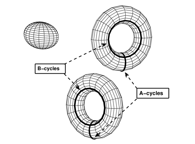
Figure 1: A multiply connected domain $D$, consisting of three components (two of genus 1 and one of genus 0), with exterior $\Omega$. Cutting along the surfaces bounded by the “A-cycle” from $D$ makes it simply connected. Adding the surfaces $T_{j}$ bounded by the B-cycles makes $\Omega\setminus D$ simply connected.

Definition 2.

Let $\Gamma_{j}$ denote a component of the boundary $\Gamma$. If

$$\int_{\Gamma_{j}}f(\boldsymbol{x})dA(\boldsymbol{x})=0$$

we refer to it as having mean zero on that component. We denote by $\mathcal{M}_{\Gamma,0}$ the set of pairs of functions $(f,g)$ on $\Gamma$ with mean zero on every component.

Lemma 1 (The mean zero condition).

Let $(r,q)$ be generalized Debye sources defined on a boundary $\Gamma$. Then $(r,q)\in\mathcal{M}_{\Gamma,0}$.

This is proven in section 6.2 (see eqs. (89) and (90)).

In multiply connected domains, the Helmholtz decomposition (20) is incomplete. From Hodge theory, however, we can write a surface vector field $\boldsymbol{j}$ as an orthogonal decomposition (in $L_{2}$), the Hodge-Helmholtz decomposition:

$$\boldsymbol{j} =\boldsymbol{j}_{R}+\boldsymbol{j}_{H}$$ (22)

$$\boldsymbol{j}_{R} =\nabla_{\Gamma}\Psi+\boldsymbol{n}\times\nabla_{\Gamma}\Psi_{m}$$

for some $\Psi,\Psi_{m}$, where $\boldsymbol{j}_{H}$ satisfies

$$\nabla_{\Gamma}\cdot\boldsymbol{j}_{H}=0,\quad\nabla_{\Gamma}\cdot(\boldsymbol{n}\times\boldsymbol{j}_{H})=0.$$

See Appendix A.3 and [29]. Such vector fields are called harmonic vector fields (dual to harmonic 1-forms). We let

$$\boldsymbol{m}_{R} = \boldsymbol{n}\times\boldsymbol{j}_{R}$$

$$\boldsymbol{m}_{H} = \boldsymbol{n}\times\boldsymbol{j}_{H}$$

and (as before)

$$\boldsymbol{m}=\boldsymbol{n}\times\boldsymbol{j}\,.$$

Harmonic vector fields arise, in essence, because the Laplace-Beltrami operator on vector fields

$$\Delta_{\Gamma}^{1}\boldsymbol{j}\equiv\nabla_{\Gamma}\nabla_{\Gamma}\cdot\boldsymbol{j}-\boldsymbol{n}\times\nabla_{\Gamma}\nabla_{\Gamma}\cdot(\boldsymbol{n}\times\boldsymbol{j}),$$ (23)

has a non-trivial nullspace on multiply connected surfaces. The dimension of the nullspace of $\Delta_{\Gamma}^{1}$ is equal to twice the genus, $g,$ of the surface. We may, therefore, choose harmonic vector fields $\{\boldsymbol{j}_{H}^{l}\,|\,l=1,\dots,2g\},$ which form an orthogonal basis,w.r.t. $L^{2}(\Gamma),$ for this nullspace. In the multiply connected case, we can then define the harmonic components of $\boldsymbol{j}$ and $\boldsymbol{m}$ by

$$\boldsymbol{j}_{H} =\sum_{l=1}^{2g}c_{l}\boldsymbol{j}_{H}^{l}$$ (24)

$$\boldsymbol{m}_{H} =\boldsymbol{n}\times\boldsymbol{j}_{H}\,.$$

The space of harmonic vector fields will be denoted $\mathcal{H}^{1}(\Gamma)$.

Given that the Laplace-Beltrami operator is not invertible, one must be careful in defining $\Psi$ and $\Psi_{m}$. From Hodge theory, however, we know that it is invertible as a map from the space of mean zero functions $\mathcal{M}_{\Gamma,0}$ to itself. We denote by $R_{0}$ the partial inverse of $\Delta_{\Gamma}$ acting on this space. Thus, we replace (21) with

$$\Psi = ikR_{0}r$$ (25)

$$\Psi_{m} = -ikR_{0}q\,,$$

where $r,q$ are the generalized Debye sources.

Example 1.

Consider a torus in $\mathbb{R}^{3}$, parametrized by

$$\boldsymbol{x}(s,t)=[(R+r\cos t)\cos s,(R+r\cos t)\sin s,r\sin t]\,,$$

with the $z$-axis as the axis of symmetry. A straightforward calculation shows that

$$\boldsymbol{j}^{1}_{H}=\frac{1}{(R+r\cos t)^{2}}\frac{\partial\boldsymbol{x}(s,t)}{\partial s}$$

and

$$\boldsymbol{j}^{2}_{H}=\boldsymbol{n}\times\boldsymbol{j}^{1}_{H}$$

are both harmonic vector fields. Since the genus of a torus is 1, they form a basis for the two-dimensional space of harmonic vector fields on the surface.

Remark 2.

Much of the formal analysis in this paper is simplified through the use of differential forms and homology theory. In order to be accessible to a broader audience, however, we state the main results using the notation of vector calculus and defer most proofs to Sections 6 and 7, where we do make use of the language and power of this theory.

2 Uniqueness Theorems for Exterior Electromagnetic Fields

Let us denote by $\overline{\mathbb{C}_{+}}$ the closed upper half plane:

$$\overline{\mathbb{C}_{+}}=\{z\in\mathbb{C}:\>\operatorname{Im}z\geq 0\}.$$

Definition 3.

A solution to the time harmonic Maxwell equations in $\Omega$ that satisfies the Silver-Müller radiation condition will be referred to as an outgoing solution.

That an outgoing solution to THME([)$k$] is determined by either the tangential components of the electric or magnetic fields is classical [8]:

Theorem 1.

Suppose that $(\boldsymbol{E},\boldsymbol{H})$ is an outgoing solution to the THME([)$k$] in an exterior region $\Omega$ for nonzero $k\in\overline{\mathbb{C}_{+}}.$ If either $\boldsymbol{n}\times\boldsymbol{E}$ or $\boldsymbol{n}\times\boldsymbol{H}$ vanishes on $\Gamma$, then the solution is identically zero in $\Omega.$

Although we will eventually address the problem of scattering from a perfect conductor ($\boldsymbol{n}\times\boldsymbol{E}=0$), we turn our attention for the moment to the Maxwell equations in exterior domains with normal components specified on the boundary. While this is not a standard physical boundary value problem, there is prior work on uniqueness and it is a natural starting point for the analysis of symmetric representations of the fields.

Theorem 2.

[Yee, 1970]. Let $(\boldsymbol{E},\boldsymbol{H})$ be an outgoing solution to the THME([)$k$] in an exterior region $\Omega$ for nonzero $k\in\overline{\mathbb{C}_{+}}.$ Suppose $\Gamma$ is simply connected, and that

$$\boldsymbol{n}\cdot\boldsymbol{E}\upharpoonright_{\Gamma}=0\ ,\ \boldsymbol{n}\cdot\boldsymbol{H}\upharpoonright_{\Gamma}=0\,.$$

Then $\boldsymbol{E}=\boldsymbol{H}=0\quad\hbox{in $\Omega$}.$

When the boundary has non-trivial topology, a rather subtle argument shows that, in general, this is not true. In particular, if the sum of the genera of the boundary components of the exterior domain is $g>0,$ then for all frequencies with non-negative imaginary part, there is a $2g$-dimensional space of outgoing solutions to the THME with vanishing normal components. The existence of these fields was proven by Kress (Theorem 3 below).

Remark 3.

In the static (harmonic) case, this fact has been known for decades [30]. More precisely, at $k=0$, the THME separate into the system

$$\nabla\cdot\boldsymbol{E}=0,\ \nabla\times\boldsymbol{E}=0\qquad\nabla\cdot\boldsymbol{H}=0,\ \nabla\times\boldsymbol{H}=0\,,$$

solutions to which are called harmonic vector fields (if they decay at infinity). When their normal components vanish on the boundary, they are called harmonic Neumann fields. If their tangential components vanish, they are called harmonic Dirichlet fields.

Theorem 3.

[Kress, 1986 [15]]. Suppose that $(\boldsymbol{E},\boldsymbol{H})$ is an outgoing solution to the THME([)$k$] in the exterior region $\Omega,$ for nonzero $k\in\overline{\mathbb{C}_{+}}.$ If every component of the boundary $\Gamma$ is simply connected, then the solution is determined by the normal components $\boldsymbol{n}\cdot\boldsymbol{E}\upharpoonright_{\Gamma}$ and $\boldsymbol{n}\cdot\boldsymbol{H}\upharpoonright_{\Gamma}.$ If the sum of the genera of the components of $\Gamma$ equals $g>0,$ then there is a subspace of outgoing solutions to THME([)$k$] with

$$\boldsymbol{n}\cdot\boldsymbol{E}\upharpoonright_{\Gamma}=0\text{ and }\boldsymbol{n}\cdot\boldsymbol{H}\upharpoonright_{\Gamma}=0$$ (26)

of dimension exactly $2g.$

Lemma 2.

[Kress, 1986 [15]]. Let $(\boldsymbol{E},\boldsymbol{H})$ be a solution to the THME([)$k$] for nonzero $k\in\overline{\mathbb{C}_{+}},$ in a region $\Omega$ with a smooth bounded boundary $\Gamma$. Then the normal components $(\boldsymbol{n}\cdot\boldsymbol{E},\boldsymbol{n}\cdot\boldsymbol{H})$ lie in $\mathcal{M}_{\Gamma,0}$.

Corollary 1.

[Kress, 1986 [15]]. Suppose that $(\boldsymbol{E},\boldsymbol{H})$ is an outgoing solution to the THME([)$k$] with $k\in\overline{\mathbb{C}_{+}}$ and satisfying

$$\boldsymbol{n}\cdot\boldsymbol{E}\upharpoonright_{\Gamma}=f\text{ and }\boldsymbol{n}\cdot\boldsymbol{H}\upharpoonright_{\Gamma}=h$$

where $f,h\in\mathcal{M}_{\Gamma,0}$ are Hölder continuous. Then $(\boldsymbol{E},\boldsymbol{H})$ are uniquely determined subject to the specification of their circulations on the A-cycles (see Fig. 1):

$$\int_{A_{j}}{\bf\tau}\cdot\boldsymbol{E}\,ds=p_{j}\text{ and }\int_{A_{j}}{\bf\tau}\cdot\boldsymbol{H}\,ds=q_{j}\,,$$ (27)

where $p_{j},q_{j}\in\mathbb{C}$ are given numbers.

Remark 4.

We call solutions to THME([)$k$] that satisfy (26) $k$-Neumann fields, and denote the space of such solutions by $\mathcal{H}_{k}(\Omega).$ The conditions in Corollary 1 are familiar from the static (zero frequency) case, where $g$ conditions must be specified for each of $\boldsymbol{E}$ and $\boldsymbol{H}$ separately, since the equations are uncoupled. For nonzero $k$, this symmetry is not required. We provide a different proof of existence in Theorem 11 and a somewhat more general analysis of uniqueness in section 6.1.

Our representation also provides an effective means for numerically computing the $k$-Neumann fields. These solutions will be needed in solving the problem of scattering from a mutiply-connected perfect conductor.

First, however, we need to recall some classical facts about layer potentials.

3 Jump Relations and Boundary Values of the Potentials

In order to use the integral representations discussed above to solve boundary value problems, we need to find expressions for the restrictions of $\boldsymbol{E}$ and $\boldsymbol{H}$ to the boundary, in terms of the various potentials. In this section we collect the relevant results. Recall that $\Gamma\hookrightarrow\mathbb{R}^{3}$ is a smooth, bounded surface (possibly disconnected). The unbounded component of $\mathbb{R}^{3}\setminus\Gamma$ which we have denoted by $\Omega,$ will be referred to as the “$+$” side of the boundary. The domain $D$ (the union of the bounded components) will be referred to as the “$-$” side. We use $\boldsymbol{n}$ to denote the unit normal vector field along $\Gamma,$ pointing into the unbounded component.

The relevant limits are given in the following lemma, proofs of which can be found, for example, in [8].

Lemma 3.

Let $\boldsymbol{A}$ and $\phi$ denote the vector and scalar potentials in (18) and let $\Gamma$ be a smooth bounded surface in $\mathbb{R}^{3}.$ For $\boldsymbol{x}_{0}\in\Gamma,$ let ${\boldsymbol{x}\to\boldsymbol{x}_{0}^{\pm}}$ indicate approach from $\Omega$ ($+$) or $D$ ($-$), respectively, and let $\boldsymbol{n}_{0}$ denote the normal at $\boldsymbol{x}_{0}$, with $\frac{\partial}{\partial n_{0}}$ the normal derivative at $\boldsymbol{x}_{0}$.. Then, for the scalar potential, we have

$$\lim_{\boldsymbol{x}\to\boldsymbol{x}_{0}^{\pm}}\boldsymbol{n}\cdot\nabla\phi_{\pm}(\boldsymbol{x}) =\mp\frac{1}{2}r(\boldsymbol{x}_{0})+K_{0}[r](\boldsymbol{x}_{0})$$ (28)

$$\lim_{\boldsymbol{x}\to\boldsymbol{x}_{0}^{\pm}}\boldsymbol{n}\times\nabla\phi_{\pm}(\boldsymbol{x}) =K_{1}[r](\boldsymbol{x}_{0}),$$

where

$$K_{0}[r](\boldsymbol{x}_{0}) =\int_{\Gamma}\frac{\partial g_{k}}{\partial n_{0}}(\boldsymbol{x}_{0}-\boldsymbol{x})\,r(\boldsymbol{x})\,dA(\boldsymbol{x})$$

$$K_{1}[r](\boldsymbol{x}_{0}) =\boldsymbol{n}_{0}\times\nabla\int_{\Gamma}g_{k}(\boldsymbol{x}_{0}-\boldsymbol{x})\,r(\boldsymbol{x})\,dA(\boldsymbol{x})\,,$$

$K_{0}$ is an integral operator of order $-1$ and $K_{1}$ is an integral operator of order $0$, which is defined in a principal value sense.

For the vector potential we have

$$\lim_{\boldsymbol{x}\to\boldsymbol{x}_{0}^{\pm}}\boldsymbol{n}\cdot\boldsymbol{A}_{\pm}(\boldsymbol{x}) =K_{2,n}[\boldsymbol{j}](\boldsymbol{x}_{0}),$$ (29)

$$\lim_{\boldsymbol{x}\to\boldsymbol{x}_{0}^{\pm}}\boldsymbol{n}\times\boldsymbol{A}_{\pm}(\boldsymbol{x}) =K_{2,t}[r](\boldsymbol{x}_{0}),$$

where

$$K_{2,n}[\boldsymbol{j}](\boldsymbol{x}_{0}) =\int_{\Gamma}g_{k}(\boldsymbol{x}_{0}-\boldsymbol{x})\,(\boldsymbol{n}_{0}\cdot\boldsymbol{j}(\boldsymbol{x}))\,dA(\boldsymbol{x})\,,$$

$$K_{2,t}[\boldsymbol{j}](\boldsymbol{x}_{0}) =\int_{\Gamma}g_{k}(\boldsymbol{x}_{0}-\boldsymbol{x})\,(\boldsymbol{n}_{0}\times\boldsymbol{j}(\boldsymbol{x}))\,dA(\boldsymbol{x})\,.$$

$K_{2,n}$ and $K_{2,t}$ are both integral operators of order $-1$.

The vector potential also satisfies

$$\lim_{\boldsymbol{x}\to\boldsymbol{x}_{0}^{\pm}}\boldsymbol{n}\cdot\nabla\times\boldsymbol{A}_{\pm}(\boldsymbol{x}) =K_{3}[\boldsymbol{j}](\boldsymbol{x}_{0})$$ (30)

$$\lim_{\boldsymbol{x}\to\boldsymbol{x}_{0}^{\pm}}\boldsymbol{n}\times\nabla\times\boldsymbol{A}_{\pm}(\boldsymbol{x}) =\pm\frac{1}{2}\boldsymbol{j}(\boldsymbol{x}_{0})+K_{4}[\boldsymbol{j}](\boldsymbol{x}_{0})\,,$$

where

$$K_{3}[\boldsymbol{j}](\boldsymbol{x}_{0}) =\int_{\Gamma}\nabla g_{k}(\boldsymbol{x}_{0}-\boldsymbol{x})\cdot(\boldsymbol{j}(\boldsymbol{x})\times\boldsymbol{n}_{0})\,dA(\boldsymbol{x})\,,$$

$$K_{4}[\boldsymbol{j}](\boldsymbol{x}_{0}) =\int_{\Gamma}\left[\nabla g_{k}(\boldsymbol{x}_{0}-\boldsymbol{x})\,(\boldsymbol{j}(\boldsymbol{x})\cdot\boldsymbol{n}_{0})-\frac{\partial g_{k}}{\partial n_{0}}(\boldsymbol{x}_{0}-\boldsymbol{x})\,\boldsymbol{j}(\boldsymbol{x})\right]\,dA(\boldsymbol{x})\,.$$

$K_{3}$ is an integral operator of order $0$. $K_{4}$ is an integral operator of order $-1$.

Proof.

These results follow from classical potential theory, the observation that the kernels in $K_{2,n}$ and $K_{2,t}$ are weakly singular, and the fact that, at the singular point $\boldsymbol{x}_{0}=\boldsymbol{x}$ in $K_{4}$, $\boldsymbol{n}_{0}$ is orthogonal to $\boldsymbol{j}(\boldsymbol{x})$). ∎

Remark 5.

We have abused notation slightly in the preceding Lemma. The operators are functions of the Helmholtz parameter $k$. When the explicit dependence is relevant, we will occasionally write $K_{0}(k),K_{1}(k),...,K_{4}(k)$ instead.

The limits of the anti-potentials $\boldsymbol{A}_{m}$ and $\phi_{m}$ are analogous. Recall, however, that we have chosen not to work with $\boldsymbol{j}$ and $\boldsymbol{m}$ as unknowns, but rather the generalized Debye sources $r,q$ complemented by the harmonic vector fields. $\boldsymbol{j}$ and $\boldsymbol{m}$ are computed from

$$\boldsymbol{j}=\nabla_{\Gamma}\Psi+\nabla_{\Gamma}\times(\boldsymbol{n}\Psi_{m})+\boldsymbol{j}_{H}$$

$$\boldsymbol{m}=\boldsymbol{n}\times\boldsymbol{j}$$

where $\Psi$ and $\Psi_{m}$ satisfy the Laplace-Beltrami equations (25) with $r,q$ viewed as source data.

Lemma 4.

The integral operators $K_{2},K_{3}$ and $K_{4}$ are all of order $-1$ or $-2$, and hence compact, when viewed as operators acting on $r,q$.

Proof.

This follows immediately from Lemma 3 and the fact that $\boldsymbol{j}$, $\boldsymbol{m}$ are of order $-1$ in terms of $(r,q)$. ∎

From Lemma 3, we obtain the following jump relations:

Corollary 2.

Suppose that the fields $\boldsymbol{E},\boldsymbol{H},$ are defined in terms of potentials and anti-potentials. Then they satisfy

$$\begin{matrix}\boldsymbol{n}\cdot(\boldsymbol{E}_{+}-\boldsymbol{E}_{-})=r\\ \boldsymbol{n}\cdot(\boldsymbol{H}_{+}-\boldsymbol{H}_{-})=q\end{matrix}\qquad\begin{matrix}\boldsymbol{n}\times(\boldsymbol{E}_{+}-\boldsymbol{E}_{-})=-\boldsymbol{m}\\ \boldsymbol{n}\times(\boldsymbol{H}_{+}-\boldsymbol{H}_{-})=\boldsymbol{j}\end{matrix}\,.$$ (31)

4 The Maxwell Equations with Normal Components Specified

We note that, for $k\in\overline{\mathbb{C}_{+}}$, the fundamental solution

$$g_{k}(\boldsymbol{x})=\frac{e^{ik|\boldsymbol{x}|}}{4\pi|\boldsymbol{x}|}$$ (32)

is outgoing; that is, it satisfies the Silver-Müller radiation condition. Thus, all of the corresponding potentials defined over bounded regions are outgoing as well.

Theorem 4.

Let $\boldsymbol{E}$ and $\boldsymbol{H}$ be outgoing fields represented in terms of Debye sources $(r,q)$ and currents $\boldsymbol{j},\boldsymbol{m}$. Then the limiting values of their normal components are given by the following integral representation for $\boldsymbol{x}_{0}\in\Gamma$.

$$\lim_{\boldsymbol{x}\to\boldsymbol{x}_{0}^{\pm}}\left(\begin{matrix}\boldsymbol{E}\cdot\boldsymbol{n}\\ \boldsymbol{H}\cdot\boldsymbol{n}\end{matrix}\right)=\\ \left(\begin{matrix}\pm\frac{1}{2}I-K_{0}&0\\ 0&\mp\frac{1}{2}I+K_{0}\end{matrix}\right)\left(\begin{matrix}r\\ q\end{matrix}\right)+\left(\begin{matrix}ikK_{2,n}&-K_{3}\\ K_{3}&ikK_{2,n}\end{matrix}\right)\left(\begin{matrix}\boldsymbol{j}\\ \boldsymbol{m}\end{matrix}\right)\,,$$ (33)

where $I$ denotes the identity operator. If we assume that $\boldsymbol{j}=\boldsymbol{j}_{R}(r,q,k)$ and $\boldsymbol{m}=\boldsymbol{n}\times\boldsymbol{j},$ then these are Fredholm integral operators of the second kind in the generalized Debye sources $(r,q)$. As $k$ tends to zero, this representation converges to

$$\lim_{\boldsymbol{x}\to\boldsymbol{x}_{0}^{\pm}}\left(\begin{matrix}\boldsymbol{E}\cdot\boldsymbol{n}\\ \boldsymbol{H}\cdot\boldsymbol{n}\end{matrix}\right)=\\ \left(\begin{matrix}\pm\frac{1}{2}I-K_{0}(0)&0\\ 0&\mp\frac{1}{2}I+K_{0}(0)\end{matrix}\right)\left(\begin{matrix}r\\ q\end{matrix}\right)$$ (34)

The equation $[-I+2K_{0}(0)]f=h$ is uniquely solvable for all $h,$ and the equation $[I+2K_{0}(0)]f=h$ for all $h$ of mean zero.

Proof.

The equations follow from the formulæ in the previous section. The solvability properties of $I\pm 2K_{0}(0)$ are classical and can be found in [8]. ∎

Definition 4.

We let $\mathcal{N}^{\pm}(k)$ denote the operator on the right hand side of (33), with $\mathcal{N}^{\pm}_{\boldsymbol{E}}(k)$ the first row and $\mathcal{N}^{\pm}_{\boldsymbol{H}}(k)$ the second.

If we seek to impose the boundary conditions $\boldsymbol{E}\cdot\boldsymbol{n}\upharpoonright_{\Gamma}=f$, $\boldsymbol{H}\cdot\boldsymbol{n}\upharpoonright_{\Gamma}=h$, then we obtain the following system of equations, which is analytic in $k.$

$$\left(\begin{matrix}\pm\frac{1}{2}I-K_{0}&0\\ 0&\mp\frac{1}{2}I+K_{0}\end{matrix}\right)\left(\begin{matrix}r\\ q\end{matrix}\right)+\left(\begin{matrix}ikK_{2,n}&-K_{3}\\ K_{3}&ikK_{2,n}\end{matrix}\right)\left(\begin{matrix}\boldsymbol{j}\\ \boldsymbol{m}\end{matrix}\right)\,=\left(\begin{matrix}f\\ h\end{matrix}\right)$$ (35)

When $\boldsymbol{j}=\boldsymbol{j}_{R}(r,q,k)$ and $\boldsymbol{m}=\boldsymbol{n}\times\boldsymbol{j}$ are obtained from the Debye sources via (25), we denote the left-hand side of (35) by $\mathcal{N}^{\pm}(k)\left(r,q\right)$ and observe that it is a compact perturbation of the operator $J_{\pm}(0)$ where

$$J_{\pm}(k)=\left(\begin{matrix}\pm\frac{1}{2}I-K_{0}(k)&0\\ 0&\mp\frac{1}{2}I+K_{0}(k)\end{matrix}\right).$$ (36)

Theorem 5.

Let $(f,h)\in\mathcal{M}_{\Gamma,0}.$ For $k\notin E_{+},$ a discrete set in the complex plane, the equation

$$\mathcal{N}^{+}(k)(r,q)=(f,h)$$ (37)

has a unique solution. The outgoing solution of the THME([)$k$] defined by this data satisfies

$$\boldsymbol{E}_{+}\cdot\boldsymbol{n}\upharpoonright_{\Gamma}=f\quad\boldsymbol{H}_{+}\cdot\boldsymbol{n}\upharpoonright_{\Gamma}=h.$$ (38)

Proof.

We know from Theorem 4 that the operator $J_{+}(0)$ is invertible. By analytic Fredholm theory, therefore, we know that there is a discrete set $E_{+}\in\mathbb{C}$ so that for $k\notin E_{+}$, $\mathcal{N}^{+}(k)$ is also invertible. The result now follows from the fact that $(r,q)\in\mathcal{M}_{\Gamma,0}$ (Lemma 1) and that $(f,h)\in\mathcal{M}_{\Gamma,0}$ (Lemma 2), so that

$$\mathcal{N}^{+}(k):\mathcal{M}_{\Gamma,0}\rightarrow\mathcal{M}_{\Gamma,0}.$$

∎

Corollary 3.

When $\Gamma$ is simply connected, the Fredholm equation (37) provides a unique solution to the THME([)$k$] for any $k\in\overline{\mathbb{C}_{+}}$.

Proof.

This follows immediately from Theorem 5 and the fact that $E_{+}$ lies in the complex lower half-plane, as follows from Corollary 4 in Section 7. ∎

Remark 6.

The problem of solving the THME with specified normal components was previously analyzed by Gülzow [12], who constructed a hypersingular integral equation method. Using generalized Debye sources instead leads to a well-conditioned integral equation of the second kind. In the multiply connected case, Theorem 5 shows that the problem of scattering with normal components specified is invertible, if the solution is sought with zero projection onto the harmonic vector fields. The extra conditions in Kress’ result (Corollary 1) force uniqueness on $\boldsymbol{j}_{H}$ by specifying $g$ conditions on the circulation of $\boldsymbol{E}$ and $g$ conditions on the circulation of $\boldsymbol{H}$, where $g$ is the genus of $\Gamma$. In fact, any set of $2g$ conditions that uniquely determines the harmonic component of the current, $\boldsymbol{j}_{H}$, will suffice. (see Theorems 9 and 11).

5 The Perfect Conductor

We turn now to the problem of scattering from a perfect conductor, which requires an analysis of the tangential components of $\boldsymbol{E}$ and $\boldsymbol{H}$. These are easily expressed in terms of potentials using Lemma 3.

Theorem 6.

Let $\boldsymbol{x}_{0}\in\Gamma$. The limiting values of the tangential components of $\boldsymbol{E},\boldsymbol{H}$, in terms of potentials and antipotentials, are given by

$$\lim_{\boldsymbol{x}\to\boldsymbol{x}_{0}^{\pm}}\left(\begin{matrix}\boldsymbol{n}\times\boldsymbol{E}\\ \boldsymbol{n}\times\boldsymbol{H}\end{matrix}\right)=\\ \frac{1}{2}\left(\begin{matrix}\pm\boldsymbol{m}\\ \mp\boldsymbol{j}\end{matrix}\right)+\left(\begin{matrix}-K_{1}&0&ikK_{2,t}&-K_{4}\\ 0&-K_{1}&K_{4}&ikK_{2,t}\end{matrix}\right)\left(\begin{matrix}r\\ q\\ \boldsymbol{j}\\ \boldsymbol{m}\end{matrix}\right).$$ (39)

where $K_{1},K_{2,t},K_{4}$ are defined in Lemma 3.

Definition 5.

In the sequel we denote the operator on the right hand side of (39) as $\mathcal{T}^{\pm}(k).$ We use $\mathcal{T}^{\pm}_{\boldsymbol{E}}(k)$ to denote the first row, and $\mathcal{T}^{\pm}_{\boldsymbol{H}}(k)$ to denote the second.

For scattering from a perfect conductor, let us recall that both (8) and (9) must hold on $\Gamma$. As noted in the introduction, the EFIE approach involves imposing (8) using only the classical vector and scalar potentials, $\boldsymbol{A}$ and $\phi$, with the physical current $\boldsymbol{J}$ as the unknown. This leads to an integral equation on $\Gamma$ with a hypersingular kernel that has interior resonances and suffers from low-frequency breakdown. To avoid these difficulties, we turn again to the Debye sources. A nonstandard feature of our approach is that we will extract only one scalar equation from the tangential conditions on the $\boldsymbol{E}$ field and couple it to the normal condition (9) satisfied by $\boldsymbol{H}$.

5.1 The hybrid system

The operator defining the tangential components of $\boldsymbol{E}_{\pm}$ is given by

$$\mathcal{T}^{\pm}_{\boldsymbol{E}}(k)\left(\begin{matrix}r\\ q\\ \boldsymbol{j}\\ \boldsymbol{m}\end{matrix}\right)=\pm\frac{1}{2}\boldsymbol{m}+\left(\begin{matrix}-K_{1}&0&ikK_{2,t}&-K_{4}\end{matrix}\right)\left(\begin{matrix}r\\ q\\ \boldsymbol{j}\\ \boldsymbol{m}\end{matrix}\right).$$ (40)

If we restrict to $\boldsymbol{j}=\boldsymbol{j}_{R}(r,q,k),$ and $\boldsymbol{m}=\boldsymbol{n}\times\boldsymbol{j},$ then, acting on $(r,q)\in\mathcal{M}_{\Gamma,0},$ the only term of non-negative order is $-K_{1}r.$ We use $\mathcal{T}^{\pm}_{\boldsymbol{E}}(k)(r,q)$ to denote this operator restricted to this subspace of data. In order to recast $K_{1}$ in (40) as a Fredholm operator of the second kind, it is convenient to multiply it by a left parametrix, based on the following standard result.

Lemma 5.

Let $\Gamma\subset\mathbb{R}^{3}$ be a smooth, connected closed surface, let $\boldsymbol{x}_{0}\in\Gamma$, and let $G_{0}$ denote the single layer potential operator based on the Green’s function for the Laplace equation:

$$G_{0}[f](\boldsymbol{x}_{0})=\int_{\Gamma}g_{0}(\boldsymbol{x}-\boldsymbol{x}_{0})f(\boldsymbol{x})\,dA(\boldsymbol{x})\,,$$ (41)

and let $\phi$ denote the usual scalar potential with density $r$. Then

$$\lim_{\boldsymbol{x}\to\boldsymbol{x}_{0}^{\pm}}G_{0}[\Delta_{\Gamma}\phi](\boldsymbol{x})=\frac{1}{4}r(\boldsymbol{x}_{0})+\widetilde{K_{1}}(\boldsymbol{x}_{0})\,$$ (42)

where $\widetilde{K_{1}}$ is a compact operator.

Proof.

To see this, we observe that the surface Laplacian satisfies the identity

$$\Delta_{\Gamma}\phi=\Delta\phi-2H\frac{\partial\phi}{\partial n}-\frac{\partial^{2}\phi}{\partial n^{2}}\,,$$

where $H$ denotes mean curvature (see, for example, [21]). Since $\Delta\phi=-k^{2}\phi$ (by construction), we have

$$\Delta_{\Gamma}\phi=-k^{2}\phi-2H\frac{\partial\phi}{\partial n}-\frac{\partial^{2}\phi}{\partial n^{2}}\,.$$ (43)

The composition of $G_{0}$ with the first two terms on the right-hand side of (43) are of order $-2$ and $-1$, respectively, hence compact. It is a classical result (a Calderon relation) that the composition of a single layer potential with the second normal derivative of $\phi$ yields a compact perturbation of $\frac{1}{4}I$ [21]:

$$\lim_{\boldsymbol{x}\to\boldsymbol{x}_{0}^{\pm}}G_{0}[\frac{\partial^{2}\phi}{\partial n^{2}}](\boldsymbol{x})=\frac{1}{4}r(\boldsymbol{x}_{0})+D^{2}[r](\boldsymbol{x}_{0})\,$$

where

$$D[r](\boldsymbol{x}_{0})=\int_{\Gamma}\frac{\partial g_{k}}{\partial n_{x}}(\boldsymbol{x}_{0}-\boldsymbol{x})\,r(\boldsymbol{x})\,dA(\boldsymbol{x})\,.$$

Here $\boldsymbol{n}_{\boldsymbol{x}}$ denotes the normal at $\boldsymbol{x}$, and $\frac{\partial}{\partial n_{x}}$ denotes the normal derivative at $\boldsymbol{x}$. $D$ is the usual double layer potential, which is the adjoint of $K_{0}$. Since $D$ is an operator of order $-1$, the result follows. ∎

Lemma 6.

Let $\Gamma\subset\mathbb{R}^{3}$ be a smooth, connected closed surface, let $\boldsymbol{x}_{0}\in\Gamma$, let $G_{0}$ denote the single layer potential operator (41). Then

$$\lim_{\boldsymbol{x}\to\boldsymbol{x}_{0}^{\pm}}G_{0}\nabla_{\Gamma}\cdot[\boldsymbol{n}\times\mathcal{T}^{\pm}_{\boldsymbol{E}}(k)]\left(\begin{matrix}r\\ q\end{matrix}\right)\,=-\frac{1}{4}r(\boldsymbol{x}_{0})+N_{1}(k)\,\left(\begin{matrix}r\\ q\end{matrix}\right)\,,$$ (44)

where $N_{1}(k)$ is an analytic family of operators of order -1.

Proof.

The result follows from Definition 5, the fact that

$$\nabla_{\Gamma}\cdot\boldsymbol{n}\times K_{1}[r]=-\Delta_{\Gamma}\phi[r]\,,$$

and the preceding Lemma. ∎

Recalling that

$$\boldsymbol{j}_{R}(r,q,0)=0,$$

we see that

$$G_{0}\nabla_{\Gamma}\cdot[\boldsymbol{n}\times\mathcal{T}^{\pm}_{\boldsymbol{E}}](0)\left(\begin{matrix}r\\ q\end{matrix}\right)=G_{0}[\Delta_{\Gamma}G_{0}\,r].$$ (45)

If $\Gamma$ has $M$ components, then the nullspace of this operator is $M$-dimensional. It is generated by functions $r$ such that $G_{0}r$ is constant on each component of $\Gamma.$ As a consequence of Theorem 5.7 in [8], it follows that this nullspace only intersects $\mathcal{M}_{\Gamma,0}$ at $0.$

Definition 6.

Taking the integral operator in Lemma 6 and the integral operator $\mathcal{N}_{\boldsymbol{H}}$ from Definition 4, we define $\mathcal{Q}^{\pm}(k)$ as the following hybrid system of integral operators:

$$\mathcal{Q}^{\pm}(k)\left(\begin{matrix}r\\ q\end{matrix}\right)=\left(\begin{matrix}G_{0}\nabla_{\Gamma}\cdot[\boldsymbol{n}\times\mathcal{T}^{\pm}_{\boldsymbol{E}}](k)\\ \mathcal{N}_{\boldsymbol{H}}^{\pm}(k)\end{matrix}\right)\left(\begin{matrix}r\\ q\end{matrix}\right).$$ (46)

As divergences, the range of $\nabla_{\Gamma}\cdot[\boldsymbol{n}\times\mathcal{T}^{\pm}_{\boldsymbol{E}}](k)$ consists of functions of mean zero.

Proposition 1.

The family of operators $\mathcal{Q}^{\pm}(k)$ is analytic in $k$ and Fredholm of the second kind. There is a discrete subset $F_{+}\subset\mathbb{C},$ such that $\mathcal{Q}^{+}(k):\mathcal{M}_{\Gamma,0}\to\mathcal{M}_{\Gamma,1}$ is invertible for $k\notin F_{+},$ where $\mathcal{M}_{\Gamma,1}$ is the $L^{2}$-closure of

$$\{(G_{0}r,q):\>(r,q)\in\mathcal{M}_{\Gamma,0}\}.$$ (47)

Proof.

The analyticity statement is immediate from the formula. Examining $\mathcal{Q}^{\pm}(k)$ we see that

$$\mathcal{Q}^{\pm}(k)\left(\begin{matrix}r\\ q\end{matrix}\right)=\left(\begin{matrix}\frac{-1}{4}&0\\ 0&\frac{\mp 1}{2}\end{matrix}\right)\left(\begin{matrix}r\\ q\end{matrix}\right)+\widetilde{N}^{\pm}_{1}(k)\left(\begin{matrix}r\\ q\end{matrix}\right),$$ (48)

where $\widetilde{N}_{1}^{\pm}$ is an analytic family of operators of order $-1.$ Thus, $\mathcal{Q}^{\pm}(k)$ is Fredholm of the second kind. The last statement follows from the facts that $\mathcal{Q}^{+}(0):\mathcal{M}_{\Gamma,0}\to\mathcal{M}_{\Gamma,1}$ is invertible and $\mathcal{Q}^{+}(k)\mathcal{M}_{\Gamma,0}\subset\mathcal{M}_{\Gamma,1}.$ ∎

We may now state our principal result in the simply connected case.

Theorem 7.

If $\Gamma$ is simply connected, then $F_{+}$ is disjoint from the closed upper half plane. Thus, the integral equation

$$\mathcal{Q}^{+}(k)\left(\begin{matrix}r\\ q\end{matrix}\right)=\left(\begin{matrix}f\\ h\end{matrix}\right)$$ (49)

provides a unique solution to the scattering problem from a perfect conductor for any $k$ in the closed upper half plane. Here,

$$f=G_{0}\nabla_{\Gamma}\cdot[\boldsymbol{n}\times\boldsymbol{n}\times\boldsymbol{E}^{\operatorname{in}}],\qquad h=\boldsymbol{n}\cdot\boldsymbol{H}^{\operatorname{in}}\upharpoonright_{T\Gamma}.$$ (50)

This is proved as Theorem 12 in Section 7.1. We leave the discussion of applying our method in the non-simply connected case to Section 7.1.

5.2 Low Frequency Behavior in the Simply Connected Case

The representation of solutions to the THME([)$k$], using data from $\mathcal{M}_{\Gamma,0}\oplus\mathcal{H}^{1}(\Gamma),$ afforded by (83) behaves well as the frequency tends to zero. In the simply connected case we only have data from $\mathcal{M}_{\Gamma,0}.$ As $k$ tends to zero, this space of solutions tends to the orthogonal complement of the harmonic Dirichlet fields, that is outgoing harmonic fields, with vanishing tangential components on $b\Omega$, so that $\boldsymbol{E}$ and $\boldsymbol{H}$ are recovered from $-\nabla\phi$ and $-\nabla\phi_{M}$ alone. This is proven, along with the multiply connected case in Section 7.2. It is therefore apparent that $\mathcal{Q}^{+}(k)$ provides a means for finding and representing solutions to the perfect conductor problem, which has neither interior resonances, nor suffers from low frequency breakdown.

6 The Exterior Form Representation

For the remainder of this paper we represent the electric field $\boldsymbol{E}$ as a 1-form $\boldsymbol{\xi},$ and the magnetic field $\boldsymbol{H}$ as a 2-form, $\boldsymbol{\eta}.$ This choice is explained in Appendix A. If

$$\boldsymbol{E}=e_{1}\partial_{x_{1}}+e_{2}\partial_{x_{2}}+e_{3}\partial_{x_{3}}\text{ and }\boldsymbol{H}=h_{1}\partial_{x_{1}}+h_{2}\partial_{x_{2}}+h_{3}\partial_{x_{3}},$$ (51)

then

$$\begin{split}&\boldsymbol{\xi}=e_{1}dx_{1}+e_{2}dx_{2}+e_{3}dx_{3}\quad\text{ and }\\ &\boldsymbol{\eta}=h_{1}dx_{2}\wedge dx_{3}+h_{2}dx_{3}\wedge dx_{1}+h_{3}dx_{1}\wedge dx_{2}.\end{split}$$ (52)

If $\langle\cdot,\cdot\rangle$ denotes the Euclidean inner product, i.e. the metric on $\mathbb{R}^{3},$ then $\boldsymbol{\xi}$ is defined by the condition that, for every vector field $\boldsymbol{V}$ we have:

$$\langle\boldsymbol{V},\boldsymbol{E}\rangle=\boldsymbol{\xi}(\boldsymbol{V}).$$ (53)

That is, $\boldsymbol{\xi}$ is the metric dual of $\boldsymbol{E},$ and $\star\boldsymbol{\eta}$ (with $\star$ the Hodge star-operator, see Remark 8 and Appendix A.2) is the metric dual of $\boldsymbol{H}.$

The curl-part of time harmonic Maxwell’s equations takes the form:

$$d\boldsymbol{\xi}=ik\boldsymbol{\eta}\quad d^{*}\boldsymbol{\eta}=-ik\boldsymbol{\xi}.$$ (54)

For $k\neq 0,$ these equations imply the divergence equations, which take the form:

$$d^{*}\boldsymbol{\xi}=0\quad d\boldsymbol{\eta}=0.$$ (55)

An outgoing solution to the Helmholtz equation on 1-forms satisfies the analog of the Silver-Müller radiation conditions:

$$i_{\hat{\boldsymbol{x}}}d\boldsymbol{\xi}-d^{*}\boldsymbol{\xi}\,\hat{\boldsymbol{x}}\cdot d\boldsymbol{x}-ik\boldsymbol{\xi}=o\left(\frac{1}{|x|}\right),$$ (56)

where $\hat{\boldsymbol{x}}=\frac{\boldsymbol{x}}{\|\boldsymbol{x}\|}.$ A magnetic field, $\boldsymbol{\eta}$ is outgoing if $\star\boldsymbol{\eta}$ satisfies (56).

The standard integration by parts formula in electromagnetic theory is derived by considering the $L^{2}$-norm of the quantity in the radiation condition. We let $D_{R}$ denote the ball of radius $R,$ centered at $0,$ $S_{R}=bD_{R},$ and $\Omega_{R}=D_{R}\cap\Omega.$ Since the quantity in (56) is $o(|x|^{-1})$ it follows easily that

$$\lim_{R\to\infty}\int\limits_{S_{R}}\|i_{\hat{\boldsymbol{x}}}d\boldsymbol{\xi}-d^{*}\boldsymbol{\xi}\,\hat{\boldsymbol{x}}\cdot d\boldsymbol{x}-ik\boldsymbol{\xi}\|^{2}dA=0.$$ (57)

We expand the integrand to obtain that

$$\begin{split}\lim_{R\to\infty}\Bigg{[}\int\limits_{S_{R}}\left[\|i_{\hat{\boldsymbol{x}}}d\boldsymbol{\xi}-d^{*}\boldsymbol{\xi}\,\hat{\boldsymbol{x}}\cdot d\boldsymbol{x}\|^{2}+|k|^{2}\|\boldsymbol{\xi}\|^{2}\right]dA+\\ -2\operatorname{Re}\left(ik\int\limits_{S_{R}}\langle\boldsymbol{\xi},i_{\hat{\boldsymbol{x}}}d\bar{\boldsymbol{\xi}}\rangle-\langle i_{\hat{\boldsymbol{x}}}\boldsymbol{\xi},d^{*}\bar{\boldsymbol{\xi}}\rangle dA\right)\Bigg{]}=0.\end{split}$$ (58)

Using Green’s formula, we can replace the second integral with

$$2\operatorname{Im}(k)\int\limits_{\Omega_{R}}\left[\|d\boldsymbol{\xi}\|^{2}+\|d^{*}\boldsymbol{\xi}\|^{2}+|k|^{2}\|\boldsymbol{\xi}\|^{2}\right]dV+\\ 2\operatorname{Im}\left[k\int\limits_{\Gamma}\left[\langle\boldsymbol{\xi},i_{\boldsymbol{n}}d\bar{\boldsymbol{\xi}}\rangle-\langle i_{\boldsymbol{n}}\boldsymbol{\xi},d^{*}\bar{\boldsymbol{\xi}}\rangle\right]dA\right].$$ (59)

Here we use $\boldsymbol{n}$ to denote the inward pointing normal field along $\Gamma.$

Combining (58) and (59) we obtain the standard integration by parts formula for outgoing solutions to the vector Helmholtz equation:

Lemma 7.

If $\boldsymbol{\xi}$ is a 1-form defined in $\Omega$ satisfying $\Delta\boldsymbol{\xi}+k^{2}\boldsymbol{\xi}=0$ and the radiation condition (56), with $\operatorname{Im}(k)\geq 0,$ then

$$\begin{split}\lim_{R\to\infty}\Bigg{(}&2\operatorname{Im}(k)\int\limits_{\Omega_{R}}\left[\|d\boldsymbol{\xi}\|^{2}+\|d^{*}\boldsymbol{\xi}\|^{2}+|k|^{2}\|\boldsymbol{\xi}\|^{2}\right]dV+\\ \int\limits_{S_{R}}\big{[}\|i_{\hat{\boldsymbol{x}}}d\boldsymbol{\xi}-d^{*}\boldsymbol{\xi}\,\hat{\boldsymbol{x}}\cdot d\boldsymbol{x}\|^{2}&+|k|^{2}\|\boldsymbol{\xi}\|^{2}\big{]}dA\Bigg{)}=\\ -&2\operatorname{Im}\left[k\int\limits_{\Gamma}\left[\langle\boldsymbol{\xi},i_{\boldsymbol{n}}d\bar{\boldsymbol{\xi}}\rangle-\langle i_{\boldsymbol{n}}\boldsymbol{\xi},d^{*}\bar{\boldsymbol{\xi}}\rangle\right]dA\right]\end{split}$$ (60)

Remark 7.

If $(\boldsymbol{\xi},\boldsymbol{\eta})$ is a solution to the THME([)$k$] in $\Omega,$ then the outgoing radiation condition can be rewritten as

$$i_{\hat{\boldsymbol{x}}}\boldsymbol{\eta}-\boldsymbol{\xi}=o\left(\frac{1}{|x|}\right),$$ (61)

in agreement with (6).

6.1 Uniqueness for Maxwell’s Equations

If $(\boldsymbol{\xi},\boldsymbol{\eta})$ is a solution to the Maxwell system, then $d^{*}\boldsymbol{\xi}=0$ and the boundary term in (60) reduces to

$$-2\operatorname{Im}\left(k\int\limits_{\Gamma}\langle\boldsymbol{\xi},i_{\boldsymbol{n}}d\bar{\boldsymbol{\xi}}\rangle dA\right).$$ (62)

Let $\nu$ denote a 1-form defined along $\Gamma,$ which restricts to zero on $T\Gamma$ and is normalized by $\nu(\boldsymbol{n})=1.$

Remark 8.

We use $\star$ to denote a Hodge star-operator, see Appendix A.2. In much of the paper we need to distinguish between the Hodge star-operator acting on forms defined on $\mathbb{R}^{3}$ and that acting on forms defined on surfaces in $\mathbb{R}^{3}.$ We denote the $\mathbb{R}^{3}$-operator by $\star_{3},$ and a surface operator by $\star_{2}.$ Which surface is intended should be clear from the context.

If $\Gamma$ is a smooth closed surface in $\mathbb{R}^{3},$ which bounds a region $D,$ then it obtains an orientation from its embedding into $\mathbb{R}^{3}:$ let $\boldsymbol{n}$ be the outward pointing unit normal vector, and $X_{1},X_{2}$ a local oriented orthonormal frame for $T\Gamma.$ We let $\omega_{1},\omega_{2},\nu,$ be the local co-frame for $T^{*}\mathbb{R}^{3}\upharpoonright_{\Gamma},$ dual to $X_{1},X_{2},\boldsymbol{n}.$ Note, in particular that, $\omega_{1}(\boldsymbol{n})=\omega_{2}(\boldsymbol{n})=0.$ We say that the frame $(X_{1},X_{2},\boldsymbol{n})$ (or co-frame $(\omega_{1},\omega_{2},\nu)$) is adapted to $\Gamma.$ The 1-form that is the metric dual of the vector field $aX_{1}+bX_{2}$ is $a\omega_{1}+b\omega_{2}.$

The volume form on $\mathbb{R}^{3}$ and area form on $\Gamma$ are given locally by

$$dV=\omega_{1}\wedge\omega_{2}\wedge\nu\quad dA=i_{\boldsymbol{n}}dV=\omega_{1}\wedge\omega_{2}.$$ (63)

In terms of the adapted frame, the Hodge star-operator on $\mathbb{R}^{3}$ is

$$\begin{split}\star_{3}1=\omega_{1}\wedge\omega_{2}\wedge\nu&\quad\star_{3}\omega_{1}\wedge\omega_{2}\wedge\nu=1\\ \star_{3}\omega_{1}=\omega_{2}\wedge\nu\quad\star_{3}\omega_{2}&=-\omega_{1}\wedge\nu\quad\star_{3}\nu=\omega_{1}\wedge\omega_{2}\\ \star_{3}\omega_{1}\wedge\nu=-\omega_{2}\quad\star_{3}\omega_{2}\wedge\nu&=\omega_{1}\quad\star_{3}\omega_{1}\wedge\omega_{2}=\nu.\end{split}$$ (64)

The Hodge star-operator on the surface (oriented as the boundary of $D$) is given by

$$\begin{split}\star_{2}1=\omega_{1}\wedge\omega_{2}&\quad\star_{2}\omega_{1}\wedge\omega_{2}=1\\ \star_{2}\omega_{1}=\omega_{2}&\quad\star_{2}\omega_{2}=-\omega_{1}.\end{split}$$ (65)

It is useful to note that if $\boldsymbol{q}$ is a 1-form defined on $\Gamma,$ then $\star_{2}^{2}\boldsymbol{q}=-\boldsymbol{q}.$ If $\boldsymbol{v}$ is a vector field tangent to $\Gamma$ and $\omega,$ its metric dual, then $\star_{2}\omega$ is the metric dual of $\boldsymbol{n}\times\boldsymbol{v}.$

To emphasize the distinction between an exterior form acting on $T\mathbb{R}^{3}$ restricted to a surface $\Gamma\subset\mathbb{R}^{3}$ and the restriction of this form to directions tangent to $\Gamma,$ we sometimes use $\boldsymbol{\alpha}\upharpoonright_{\Gamma}$ to denote the former notion of restriction, and $\boldsymbol{\alpha}\upharpoonright_{T\Gamma},$ the latter. For a 1-form, $\boldsymbol{\alpha},$ represented along $\Gamma$ in the adapted co-frame by $\boldsymbol{\alpha}\upharpoonright_{\Gamma}=a\omega_{1}+b\omega_{2}+c\nu,$ we have

$$\boldsymbol{\alpha}\upharpoonright_{T\Gamma}\leftrightarrow a\omega_{1}+b\omega_{2}.$$ (66)

We denote this latter restriction by $\boldsymbol{\alpha}_{t}.$ We use the notation $d_{\Gamma}$ to denote the exterior differential acting on forms on $\Gamma.$

For a 2-form $\boldsymbol{\beta}\upharpoonright_{\Gamma}=a\omega_{1}\wedge\nu+b\omega_{2}\wedge\nu+c\omega_{1}\wedge\omega_{2},$ we have

$$\boldsymbol{\beta}\upharpoonright_{T\Gamma}\leftrightarrow c\omega_{1}\wedge\omega_{2}.$$ (67)

For a 3-form $\boldsymbol{\gamma},$ dimensional considerations imply that

$$\boldsymbol{\gamma}\upharpoonright_{T\Gamma}\equiv 0.$$ (68)

If $f$ is a 0-form, or scalar function, then

$$f\upharpoonright_{T\Gamma}=f\upharpoonright_{\Gamma}.$$ (69)

The definition of the inner product on forms, the fact that $\langle\nu,i_{\boldsymbol{n}}d\bar{\boldsymbol{\xi}}\rangle=0,$ and the definition of $\star_{2}$ on $\Gamma,$ imply the identity

$$-2\operatorname{Im}\left(k\int\limits_{\Gamma}\langle\boldsymbol{\xi},i_{\boldsymbol{n}}d\bar{\boldsymbol{\xi}}\rangle dA\right)=-2\operatorname{Im}\left(k\int\limits_{\Gamma}[\boldsymbol{\xi}\upharpoonright_{\Gamma}]\wedge\star_{2}[i_{\boldsymbol{n}}d\bar{\boldsymbol{\xi}}\upharpoonright_{\Gamma}]\right).$$ (70)

Using this identity and Lemma 7 we can prove the basic uniqueness theorems. Note that $\boldsymbol{\xi}$ is a 1-form so $\boldsymbol{\xi}_{t}=\boldsymbol{\xi}\upharpoonright_{T\Gamma}$ corresponds to the tangential components of $\boldsymbol{E},$ and $i_{\boldsymbol{n}}\boldsymbol{\xi}\upharpoonright_{\Gamma},$ the normal component. The magnetic field $\boldsymbol{\eta}$ is a 2-form and therefore $\boldsymbol{\eta}\upharpoonright_{T\Gamma}$ gives the normal component, and $[i_{\boldsymbol{n}}\boldsymbol{\eta}]_{t}=i_{\boldsymbol{n}}\boldsymbol{\eta}\upharpoonright_{T\Gamma},$ gives the data in the tangential components, corresponding to $n\times\boldsymbol{H}.$

We restate the classical result (Theorem 1) that an outgoing solution to THME([)$k$] is determined by either the tangential components of the electric or magnetic fields in the language of forms:

Theorem 8.

Suppose that $(\boldsymbol{\xi},\boldsymbol{\eta})$ is an outgoing solution to the THME([)$k$], in $\Omega,$ for a $k\neq 0,$ in $\overline{\mathbb{C}_{+}}.$ If either $\boldsymbol{\xi}_{t},$ or $[i_{\boldsymbol{n}}\boldsymbol{\eta}]_{t}$ vanish, then the solution is identically zero in $\Omega.$

Kress’ result (Theorem 3) on the normal components of $(\boldsymbol{\xi},\boldsymbol{\eta})$ is restated as

Theorem 9.

Suppose that $(\boldsymbol{\xi},\boldsymbol{\eta})$ is an outgoing solution to the THME([)$k$], in $\Omega,$ for a $k\neq 0,$ in $\overline{\mathbb{C}_{+}}.$ If every component of the boundary of $\Omega$ is simply connected, then the solution is determined by the normal components $i_{\boldsymbol{n}}\boldsymbol{\xi}\upharpoonright_{\Gamma}$ and $\boldsymbol{\eta}\upharpoonright_{T\Gamma}.$ If the sum of the genera of the components of $\Gamma$ equals $g>0,$ then there is a subspace of outgoing solutions to THME([)$k$] with

$$i_{\boldsymbol{n}}\boldsymbol{\xi}\upharpoonright_{\Gamma}=0\text{ and }\boldsymbol{\eta}\upharpoonright_{T\Gamma}=0$$ (71)

of dimension $2g.$

Remark 9.

As noted above, we call solutions to THME([)$k$] that satisfy (71) $k$-Neumann fields, and denote the space of such solutions by $\mathcal{H}_{k}(\Omega).$ Here we give a bound on $\dim\mathcal{H}_{k}(\Omega),$ and a novel description of the additional data needed to specify the projection into this space. Later in the paper we give a new proof that $\dim\mathcal{H}_{k}(\Omega)=2g,$ for $k$ in the closed upper half plane, $\overline{\mathbb{C}_{+}}.$ In this regard, the case $k=0$ is classical. As noted above, this result was proved in [15].

Proof.

Suppose that $i_{\boldsymbol{n}}\boldsymbol{\xi}$ and $\boldsymbol{\eta}\upharpoonright_{\Gamma}$ both vanish. Let $\boldsymbol{\alpha}=\boldsymbol{\xi}\upharpoonright_{\Gamma}$ and $\boldsymbol{\beta}=\star_{3}\boldsymbol{\eta}\upharpoonright_{\Gamma}.$ The usual properties of the exterior derivative, the hypothesis $\boldsymbol{\eta}\upharpoonright_{\Gamma}=0,$ and the equation $d\boldsymbol{\xi}=ik\boldsymbol{\eta}$ imply that

$$d_{\Gamma}\boldsymbol{\alpha}=0.$$ (72)

We can rewrite $d^{*}\boldsymbol{\eta}=-ik\boldsymbol{\xi}$ as $d\star_{3}\boldsymbol{\eta}=-ik\star_{3}\boldsymbol{\xi}.$ The hypothesis, $i_{\boldsymbol{n}}\boldsymbol{\xi}=0$ now implies that

$$d_{\Gamma}\boldsymbol{\beta}=0.$$ (73)

A calculation using a co-frame adapted to $\Gamma$ shows that

$$\star_{2}\boldsymbol{\beta}=-[i_{\boldsymbol{n}}\boldsymbol{\eta}]\upharpoonright_{\Gamma},$$ (74)

see (97). The equation $d\boldsymbol{\xi}=ik\boldsymbol{\eta}$ implies that

$$[i_{\boldsymbol{n}}d\boldsymbol{\xi}]\upharpoonright_{\Gamma}=-ik\star_{2}\boldsymbol{\beta}.$$ (75)

We can therefore express the right hand side of (70) as

$$2|k|^{2}\operatorname{Re}\left(\int\limits_{\Gamma}\boldsymbol{\alpha}\wedge\bar{\boldsymbol{\beta}}\right).$$ (76)

If $\Gamma$ is simply connected then the equation $d_{\Gamma}\boldsymbol{\alpha}=0$ implies that $\boldsymbol{\alpha}=d_{\Gamma}u.$ As $d_{\Gamma}\bar{\boldsymbol{\beta}}=0$ as well, a simple application of Stokes formula shows that

$$\int\limits_{\Gamma}d_{\Gamma}u\wedge\bar{\boldsymbol{\beta}}=0.$$ (77)

This completes the proof of the theorem when $\Gamma$ is simply connected.

For the general case, let $H^{1}_{\operatorname{dR}}(\Gamma)$ denote the De Rham cohomology group with $\dim H^{1}_{\operatorname{dR}}(\Gamma)=2g\neq 0$. We show that the space of solutions with vanishing normal components, for which the integral in (76) is non-vanishing, depends on at most $2g$ parameters. Using the wedge product, we define a pairing, $W,$ on closed 1-forms:

$$W(\eta,\omega)=\int\limits_{\Gamma}\eta\wedge\omega.$$ (78)

If $d_{\Gamma}\eta=0$ and $\omega=d_{\Gamma}u,$ then, as noted above, Stokes theorem implies that

$$W(\eta,\omega)=0.$$ (79)

Hence $W$ defines a skew-symmetric form on $H^{1}_{\operatorname{dR}}(\Gamma),$ which is well known to be non-degenerate. As the $\dim H^{1}_{\operatorname{dR}}(\Gamma)=2g,$ this observation completes the proof of the fact that $\dim\mathcal{H}_{k}(\Omega)\leq 2g.$ If the image of either $\boldsymbol{\alpha}$ or $\boldsymbol{\beta}$ in $H^{1}_{\operatorname{dR}}(\Gamma)$ vanishes, then $W(\boldsymbol{\alpha},\bar{\boldsymbol{\beta}})=0,$ which implies, as above, that the solution in $\Omega$ is zero. ∎

From this proof we see that the image of either $\boldsymbol{\alpha}$ or $\boldsymbol{\beta}$ in $H^{1}(\Gamma)$ provides data specifying a $k$-Neumann field. This should be contrasted with the data used by Kress, given in equation (27). As $\dim\mathcal{H}_{k}(\Omega)=\dim H^{1}(\Gamma),$ the maps from $\mathcal{H}_{k}(\Omega)$ to $H^{1}(\Gamma)$ defined by $(\boldsymbol{\xi},\boldsymbol{\eta})\mapsto\boldsymbol{\alpha}$ and $(\boldsymbol{\xi},\boldsymbol{\eta})\mapsto\boldsymbol{\beta}$ are both isomorphisms, when $k\neq 0.$

We complete this section by proving Lemma 2, which shows that the normal components of $(\boldsymbol{\xi},\boldsymbol{\eta}),$ a solution to THME([)$k$] with $k\neq 0,$ have vanishing mean value over every component of the boundary. While superficially this might appear analogous to the fact that the normal derivative of a harmonic function in a bounded domain has mean value over the boundary, it is actually an elementary consequence of the equations themselves and Stokes’ theorem on a closed surface.

If $k\neq 0,$ then the Maxwell equations, (54), imply that

$$\star_{3}\boldsymbol{\xi}\upharpoonright_{\Gamma}=\frac{-1}{ik}d_{\Gamma}[\star_{3}\boldsymbol{\eta}\upharpoonright_{\Gamma}]\quad\boldsymbol{\eta}\upharpoonright_{\Gamma}=\frac{1}{ik}d_{\Gamma}[\boldsymbol{\xi}\upharpoonright_{\Gamma}].$$ (80)

As

$$\star_{3}\boldsymbol{\xi}\upharpoonright_{\Gamma}=i_{\boldsymbol{n}}\boldsymbol{\xi}dA$$ (81)

the relations in (80) imply that these forms are exact and therefore Stokes’ theorem implies that a solution of THME([)$k$], with $k\neq 0$ satisfies:

$$\int\limits_{\Gamma_{m}}i_{\boldsymbol{n}}\boldsymbol{\xi}dA=\int\limits_{\Gamma_{m}}\boldsymbol{\eta}=0$$ (82)

for $m=1,\dots,M.$ Note that this is true whether the limit is taken from $\Omega$ or $D.$ This completes the proof of Lemma 2, restated as

Proposition 2.

Let $(\boldsymbol{\xi},\boldsymbol{\eta})$ be a solution to the THME([)$k$] for a $k\neq 0,$ in a region $G\subset\mathbb{R}^{3},$ with a smooth bounded boundary. The normal components $(i_{\boldsymbol{n}}\boldsymbol{\xi},i_{n}\star_{3}\boldsymbol{\eta})$ have mean zero over every component of $bG.$

6.2 Potentials and Boundary Integral Equations

We now re-express (16) in terms of exterior forms. Assuming, as before, that the time dependence is $e^{-i\omega t},$ the permittivity is $\epsilon,$ the permeabilty is $\mu,$ and $k=\omega\sqrt{\epsilon\mu};$ we set

$$\boldsymbol{\xi}=(ik\boldsymbol{\alpha}-d\phi-d^{*}\boldsymbol{\alpha}_{m})\quad\boldsymbol{\eta}=(d\boldsymbol{\alpha}+ik\boldsymbol{\alpha}_{m}+d^{*}\Phi_{m}),$$ (83)

where $\phi$ is a scalar function, $\boldsymbol{\alpha}$ a one form, $\boldsymbol{\alpha}_{m}$ a two form, and $\Phi_{m}=\phi_{m}dV,$ a three form. This representation is quite similar to what one obtains using the fundamental solution for the Dirac operator $d+d^{*},$ see [3].

In order for $(\boldsymbol{\xi},\boldsymbol{\eta})$ to satisfy the THME([)$k$], the potentials must satisfy:

$$d^{*}\boldsymbol{\alpha}=-ik\phi\quad d\boldsymbol{\alpha}_{m}=ik\Phi_{m}.$$ (84)

As before $g_{k}(x-y)$ denotes the outgoing fundamental solution for the scalar Helmholtz equation, with frequency $k.$ As discussed in the introduction, all of the potentials are expressed in terms of a pair of 1-forms $\boldsymbol{j},\boldsymbol{m}$ defined on $\Gamma,$ though in the end, we do not use $\boldsymbol{j}$ and $\boldsymbol{m}$ as the “fundamental” parameters. When we express these 1-forms in terms of the ambient basis from $\mathbb{R}^{3},$ e.g.,

$$\boldsymbol{j}=j_{1}(x)dx_{1}+j_{2}(x)dx_{2}+j_{3}(x)dx_{3},$$ (85)

we normalize with the requirement

$$i_{\boldsymbol{n}}\boldsymbol{j}=\boldsymbol{j}(\boldsymbol{n})\equiv 0.$$ (86)

These 1-forms are the metric duals of the vector fields, tangent to $\Gamma,$‘ previously denoted by $\boldsymbol{j}$ and $\boldsymbol{m}.$

The “vector” potentials are given in terms of surface integrals by setting

$$\begin{split}\boldsymbol{\alpha}&=\int\limits_{\Gamma}g_{k}(x-y)[j_{1}(y)dx_{1}+j_{2}(y)dx_{2}+j_{3}(y)dx_{3}]dA(y)\\ \boldsymbol{\alpha}_{m}&=\star_{3}\left[\int\limits_{\Gamma}g_{k}(x-y)[m_{1}(y)dx_{1}+m_{2}(y)dx_{2}+m_{3}(y)dx_{3}]dA(y)\right].\end{split}$$ (87)

Using the equations in (84) we obtain the form of the potentials defining $\phi$ and $\Phi_{m}=\phi_{m}dV,$ letting

$$\begin{split}\phi(x)&=\int\limits_{\Gamma}g_{k}(x-y)r(y)dA(y)\\ \phi_{m}(x)&=\int\limits_{\Gamma}g_{k}(x-y)q(y)dA(y),\end{split}$$ (88)

where we let

$$\frac{1}{ik}d_{\Gamma}\star_{2}\boldsymbol{j}=rdA\quad\frac{1}{ik}d_{\Gamma}\star_{2}\boldsymbol{m}=qdA.$$ (89)

The scalar functions, $(r,q)$ are, as before, the Debye sources. From this definition, and Stokes’ theorem we see that the mean values of $r$ and $q$ vanish on every connected component, $\Gamma_{j},$ of $\Gamma,$

$$\int\limits_{\Gamma_{j}}rdA=\int\limits_{\Gamma_{j}}qdA=0$$ (90)

This proves Lemma 1. It is necessary for the conditions in (89) to hold, and thus, for $(\boldsymbol{\xi},\boldsymbol{\eta})$ to satisfy the Maxwell equations.

As before, we let $\mathcal{M}_{\Gamma,0}$ denote pairs of functions $(r,q)$ defined on $\Gamma$ with mean zero on every component of $\Gamma.$ If we assume that $\boldsymbol{m}=\star_{2}\boldsymbol{j},$ (as we usually do), then, taking account of the fact that the (negative) Laplace operator on 1-forms is given by $-\Delta_{1}=d_{\Gamma}^{*}d_{\Gamma}+d_{\Gamma}d_{\Gamma}^{*},$ we obtain the relation:

$$\Delta_{1}\boldsymbol{j}=ik[d_{\Gamma}r-\star_{2}d_{\Gamma}q].$$ (91)

If the components of $\Gamma$ are all of genus zero, then equation (91) always has a unique solution. If $\Gamma$ has positive genus components, then one needs to deal with the null space of $\Delta_{1}.$

If $H^{1}_{\operatorname{dR}}(\Gamma)\neq 0,$ then the nullspace of $\Delta_{1},$ $\mathcal{H}^{1}(\Gamma),$ which agrees with the space of solutions to

$$d_{\Gamma}\boldsymbol{\alpha}=0\quad d^{*}_{\Gamma}\boldsymbol{\alpha}=0$$ (92)

is isomorphic to $H^{1}_{\operatorname{dR}}(\Gamma).$ These are the harmonic 1-forms. The right hand side in (91) is orthogonal to $\mathcal{H}^{1}(\Gamma),$ and hence lies in the range of $\Delta_{1}.$ Let $R_{1}$ denote the partial inverse of the Laplacian on 1-forms, with range orthogonal to $\mathcal{H}^{1}(\Gamma),$ and set

$$\boldsymbol{j}_{R}(r,q,k)=ikR_{1}[d_{\Gamma}r-\star_{2}d_{\Gamma}q],$$ (93)

Because the ranges of $d_{\Gamma}$ and $d^{*}_{\Gamma}$ are orthogonal to the null space of $\Delta_{1},$ this equation is solvable whether or not $r$ and $q$ satisfy the mean value condition. Note that the solution to (93) tends to zero as $k\to 0.$

Using the relations $\Delta_{1}d_{\Gamma}=d_{\Gamma}\Delta_{0},$ and $\Delta_{2}=\star_{2}\Delta_{0}\star_{2},$ we can re-express $\boldsymbol{j}_{R}$ in the form:

$$\boldsymbol{j}_{R}(r,q,k)=ik[d_{\Gamma}R_{0}r-\star_{2}d_{\Gamma}R_{0}q].$$ (94)

Here $R_{0}$ is the partial inverse of $\Delta_{0},$ which annihilates functions constant on each component of $\Gamma$ and has range equal to the set of functions with mean zero on each component of $\Gamma.$ Equation (94) shows that this approach to representing solutions of Maxwell’s equations in terms of the pair $(r,q),$ only requires an inverse for the scalar Laplacian on $\Gamma.$

For any $(r,q),$ the solution space to (91) is isomorphic to $\mathcal{H}^{1}(\Gamma).$ Adding a harmonic 1-form to $\boldsymbol{j}_{R}$ does not change $r$ and $q,$ though it changes the fields $\boldsymbol{\xi}$ and $\boldsymbol{\eta},$ and plays a central role in the discussion of $\mathcal{H}_{k}(\Omega).$ If $g\neq 0,$ then the space of outgoing solutions to THME([)$k$] is parameterized by $\mathcal{M}_{\Gamma,0}\oplus\mathcal{H}^{1}(\Gamma).$ So given data $(r,q,\boldsymbol{j}_{H})$ we often speak of the solution to the THME([)$k$] “defined” by this data. If $\boldsymbol{j}_{H}$ is missing, then it should be understood to be zero, i.e. the solution “defined by $(r,q)$,” is the solution defined by $(r,q,0)$ in the sense above.

6.3 Boundary Equations and Jump Relations

As with the vector field representation, we can take the limits of $\boldsymbol{\xi}$ and $\boldsymbol{\eta}$ in (83) as the point of evaluation approaches $\Gamma,$ and obtain boundary integral equations for the normal and tangential components of these forms. Indeed there is no necessity to rewrite these equations, we simply use $\mathcal{T}_{\boldsymbol{\xi}}^{\pm}(k)(r,q,\boldsymbol{j},\boldsymbol{m}),$ $\mathcal{T}_{\boldsymbol{\eta}}^{\pm}(k)(r,q,\boldsymbol{j},\boldsymbol{m})$ to denote the limiting tangential components and the limiting normal components are $\mathcal{N}_{\boldsymbol{\xi}}^{\pm}(k)(r,q,\boldsymbol{j},\boldsymbol{m}),$ $\mathcal{N}_{\boldsymbol{\eta}}^{\pm}(k)(r,q,\boldsymbol{j},\boldsymbol{m}).$ Keep in mind that, in the vector field representation, the tangential components are represented as the limits of $\boldsymbol{n}\times\boldsymbol{E}$ and $\boldsymbol{n}\times\boldsymbol{H},$ which correspond to $\star_{2}\boldsymbol{\xi}_{t}$ and $\star_{2}([\star_{3}\boldsymbol{\eta}]_{t}),$ respectively. For consistency, we use $\mathcal{T}_{\boldsymbol{\xi}}^{\pm},\mathcal{T}_{\boldsymbol{\eta}}^{\pm}$ to denote the boundary values of these quantities. As before, $+$ indicates the limit taken from $\Omega$ and $-$ the limit taken from $D.$ If $\boldsymbol{j}=\boldsymbol{j}_{R}(r,q,k)$ and $\boldsymbol{m}=\star_{2}\boldsymbol{j},$ then we omit them from the argument list, e.g., we use the abbreviated notation $\mathcal{T}_{\boldsymbol{\xi}}^{\pm}(k)(r,q)$ to denote $\mathcal{T}_{\boldsymbol{\xi}}^{\pm}(k)(r,q,\boldsymbol{j}_{R}(r,q,k),\star_{2}\boldsymbol{j}_{R}(r,q,k)),$ etc.

Below we use the jump relations to prove a uniqueness theorem. So it is useful to reformulate them in the form language. The magnetic field is represented by the 2-form, $\boldsymbol{\eta}=h_{1}dx_{2}\wedge dx_{3}+h_{2}dx_{3}\wedge dx_{1}+h_{3}dx_{1}\wedge dx_{2},$ so that $\star_{3}\boldsymbol{\eta}=h_{1}dx_{1}+h_{2}dx_{2}+h_{3}dx_{3}.$ The most direct way to define the normal and tangential components of $\boldsymbol{\eta}$ along $\Gamma$ is as $i_{\boldsymbol{n}}\star_{3}\boldsymbol{\eta}_{\pm}$ and $(\star_{3}\boldsymbol{\eta}_{\pm})_{t}.$ In this formulation the jump relations then take the form

$$\begin{split}i_{\boldsymbol{n}}(\boldsymbol{\xi}_{+}-\boldsymbol{\xi}_{-})=r&\quad(\boldsymbol{\xi}_{+}-\boldsymbol{\xi}_{-})_{t}=\star_{2}\boldsymbol{m}\\ i_{\boldsymbol{n}}(\star_{3}\boldsymbol{\eta}_{+}-\star_{3}\boldsymbol{\eta}_{-})=q&\quad(\star_{3}\boldsymbol{\eta}_{+}-\star_{3}\boldsymbol{\eta}_{-})_{t}=-\star_{2}\boldsymbol{j}\end{split}$$ (95)

It is also useful to calculate the relationship between $i_{\boldsymbol{n}}\boldsymbol{\eta}$ and $(\star_{3}\boldsymbol{\eta})_{t}.$ In an adapted frame $(\omega_{1},\omega_{2},\nu),$ We have

$$\boldsymbol{\eta}=a\omega_{1}\wedge\omega_{2}+b\nu\wedge\omega_{1}+c\nu\wedge\omega_{2}$$ (96)

and therefore

$$\begin{cases}i_{\boldsymbol{n}}\boldsymbol{\eta}&=b\omega_{1}+c\omega_{2}\\ (\star_{3}\boldsymbol{\eta})_{t}&=b\omega_{2}-c\omega_{1},\end{cases}\text{ which implies that}\star_{2}[i_{\boldsymbol{n}}\boldsymbol{\eta}]=(\star_{3}\boldsymbol{\eta})_{t}.$$ (97)

7 Uniqueness for the Tangential Equations

Suppose that there is a $k\in\overline{\mathbb{C}_{+}}\setminus\{0\},$ and non-trivial data $(r,q)\in\mathcal{M}_{\Gamma,0}$ and $\boldsymbol{j},$ satisfying (89), with $\boldsymbol{m}=\star_{2}\boldsymbol{j},$ so that

$$\mathcal{T}^{+}_{\boldsymbol{\xi}}(k)(r,q,\boldsymbol{j},\boldsymbol{m})=0.$$ (98)

Let $(\boldsymbol{\xi}_{\pm},\boldsymbol{\eta}_{\pm})$ be the solutions to the Maxwell equations defined by this data in the complement of $\Gamma.$ By their definition it is clear that the tangential components of $\boldsymbol{\xi}_{+}$ vanish along $\Gamma.$ As $\operatorname{Im}(k)\geq 0,$ the solution in $\Omega$ is outgoing and Theorem 8 shows that $(\boldsymbol{\xi}_{+},\boldsymbol{\eta}_{+})\equiv(0,0).$ The jump relations, (95), and the fact that $\boldsymbol{m}=\star_{2}\boldsymbol{j},$ allow us to determine the tangential boundary data for $(\boldsymbol{\xi}_{-},\boldsymbol{\eta}_{-}):$

$$\boldsymbol{\xi}_{-}\upharpoonright_{T\Gamma}=\boldsymbol{j}\quad i_{\boldsymbol{n}}\boldsymbol{\eta}_{-}\upharpoonright_{T\Gamma}=\boldsymbol{j}.$$ (99)

It is not difficult to see that the boundary condition on the Maxwell system in $D,$ implied by these relations,

$$\boldsymbol{\xi}_{-}\upharpoonright_{T\Gamma}=i_{\boldsymbol{n}}\boldsymbol{\eta}_{-}\upharpoonright_{T\Gamma},$$ (100)

is not formally self adjoint!

Observe that $d^{*}d\boldsymbol{\xi}_{-}=k^{2}\boldsymbol{\xi}_{-}$ and $i_{\boldsymbol{n}}d\boldsymbol{\xi}_{-}\upharpoonright_{\Gamma}=iki_{\boldsymbol{n}}\boldsymbol{\eta}_{-}\upharpoonright_{\Gamma}.$ Using a standard integration by parts formula, we obtain:

$$\begin{split}\int\limits_{D}(d\boldsymbol{\xi}_{-},d\boldsymbol{\xi}_{-})dV&=\int\limits_{D}(d^{*}d\boldsymbol{\xi}_{-},\boldsymbol{\xi}_{-})dV+\int\limits_{bD}(i_{\boldsymbol{n}}d\boldsymbol{\xi}_{-},\boldsymbol{\xi}_{-})dA\\ &=k^{2}\int\limits_{D}(\boldsymbol{\xi}_{-},\boldsymbol{\xi}_{-})dV+ik\int\limits_{bD}(i_{\boldsymbol{n}}\boldsymbol{\eta}_{-}\upharpoonright_{\Gamma},\boldsymbol{\xi}_{-}\upharpoonright_{\Gamma})dA.\end{split}$$ (101)

Combining this with (99) gives:

$$-ik\int\limits_{bD}(\boldsymbol{j},\boldsymbol{j})dA=k^{2}\int\limits_{D}(\boldsymbol{\xi}_{-},\boldsymbol{\xi}_{-})dV-\int\limits_{D}(d\boldsymbol{\xi}_{-},d\boldsymbol{\xi}_{-})dV.$$ (102)

We can rewrite this relation as

$$-aik=bk^{2}-c,$$ (103)

where $a,b,c$ are non-negative real numbers. If $b$ or $c$ vanishes, then it is clear that $\boldsymbol{\xi}_{-}\equiv 0.$ If $a=0,$ then $\boldsymbol{j}\equiv 0.$ For a countable set of real numbers $\{k_{j}\},$ there exist non-trivial solutions to the equations

$$d^{*}d\boldsymbol{\xi}_{-}=k_{j}^{2}\boldsymbol{\xi}_{-}\quad d^{*}\boldsymbol{\xi}_{-}=0\quad\boldsymbol{\xi}_{-}\upharpoonright_{TbD}=0.$$ (104)

In the present circumstance, however, $(r,q)$ are generalized Debye sources and therefore

$$rdA=\frac{1}{ik}d_{\Gamma}\star_{2}\boldsymbol{j}\text{ and }qdA=\frac{1}{ik}d_{\Gamma}\boldsymbol{j}.$$ (105)

If $a=0,$ then all the boundary potentials vanish, and therefore $\boldsymbol{\xi}_{-}\equiv 0$ as well.

Using the quadratic formula we see that

$$k_{\pm}=\frac{-ia\pm\sqrt{4bc-a^{2}}}{2b}.$$ (106)

As $a,b,c$ are all positive, (106) shows that $\operatorname{Im}k_{\pm}<0.$ This argument applies, mutatis mutandis to $\mathcal{T}^{+}_{\boldsymbol{\eta}}(k).$ Formula (106) and the discussion above complete the proof of the following theorem:

Theorem 10.

Assuming that $\boldsymbol{m}=\star_{2}\boldsymbol{j},$ and $(r,q)$ satisfy (89), then, for $\operatorname{Im}k\geq 0,$ $k\neq 0,$ the nullspaces of both $\mathcal{T}^{+}_{\boldsymbol{\xi}}(k)$ are $\mathcal{T}^{+}_{\boldsymbol{\eta}}(k)$ are trivial.

In the case that $\Gamma$ is simply connected this implies that $E_{+},$ the exceptional set for $\mathcal{N}^{+}(k),$ is disjoint from the closed upper half plane.

Corollary 4.

If every component of $\Gamma$ is simply connected, then, for $k$ with $\operatorname{Im}k\geq 0,$ the Fredholm operator $\mathcal{N}^{+}(k)$ is an isomorphism from $\mathcal{M}_{\Gamma,0}$ to itself. For such $k,$ the rows of $\mathcal{T}^{+}(k)$ are also surjective and hence isomorphisms.

Proof.

If $\Gamma$ is simply connected, then any 1-form $\boldsymbol{j}$ on $\Gamma$ has a unique representation as $\boldsymbol{j}=\boldsymbol{j}_{R}(r,q,k).$ We can therefore regard $\mathcal{N}^{+}(k)$ as a Fredholm system of second kind for the normal components of $(\boldsymbol{\xi}_{+},\boldsymbol{\eta}_{+})$ in terms of $(r,q).$ In this case, Theorem 9 implies that a solution $(\boldsymbol{\xi}_{+},\boldsymbol{\eta}_{+})$ of THME([)$k$], with vanishing normal components is identically zero in $\Omega.$ Hence $(\boldsymbol{\xi}_{-},\boldsymbol{\eta}_{-})$ satisfy (99), and we can therefore apply the argument leading up to Theorem 10 to prove that $E_{+}$ is disjoint from the closed upper half plane. The Fredholm alternative then implies that $\mathcal{N}^{+}(k)$ is also surjective. The surjectivity of the rows of $\mathcal{T}^{+}(k)$ is now immediate. ∎

Remark 10.

The poles of the scattering operator for the Maxwell system, defined by a self adjoint boundary condition on $\Gamma$, lie in the lower half plane. Nonetheless, it appears that the eigenvalues for the non-self adjoint boundary value problem defined by (100) are unrelated to these poles, but are simply interior resonances, familiar from more traditional representations of solutions to Maxwell’s equations (see the Introduction and Remark 15). The non-self adjointness of this BVP places the interior resonances in the lower, non-physical, half plane. This leads, in the simply connected case, to numerically effective algorithms for solving the THME([)$k$], which do not suffer from the instabilities caused by interior resonances in the physical half plane.

In the non-simply connected case we have the following theorem assuring the existence of $k$-Neumann fields.

Theorem 11.

For $k\in\overline{\mathbb{C}_{+}},$ the space of $k$-Neumann fields has dimension exactly $2g,$ and the rows of $\mathcal{T}^{+}(k)$ are surjective.

Proof.

For $k\in\overline{\mathbb{C}_{+}},$ the solutions to THME([)$k$], defined by

$$\mathcal{C}_{H}=\{(0,0,\boldsymbol{j}_{H},\star_{2}\boldsymbol{j}_{H}):\>\boldsymbol{j}_{H}\in\mathcal{H}^{1}(\Gamma)\}$$

have a trivial intersection with those defined by data in

$$\mathcal{C}_{R}=\{(r,q,\boldsymbol{j}_{R}(r,q,k),\star_{2}\boldsymbol{j}_{R}(r,q,k)):\>(r,q)\in\mathcal{M}_{\Gamma,0}\}.$$

The solutions defined by data in $\mathcal{C}_{H}$ may not themselves be $k$-Neumann fields. To find solutions in $\mathcal{H}_{k}(\Omega),$ we first use an element of $\mathcal{C}_{H}$ to construct a solution $(\boldsymbol{\xi}_{0+},\boldsymbol{\eta}_{0+}).$ If $k\notin E_{+},$ then we can solve

$$\mathcal{N}^{+}(k)\left(\begin{matrix}r\\ q\end{matrix}\right)=\left(\begin{matrix}i_{\boldsymbol{n}}\boldsymbol{\xi}_{0+}\\ i_{\boldsymbol{n}}\star_{3}\boldsymbol{\eta}_{0+}\end{matrix}\right),$$ (107)

and denote the solution of the THME([)$k$] defined by this data in $\Omega$ by $(\boldsymbol{\xi}_{1+},\boldsymbol{\eta}_{1+}).$ By Theorem 10, the difference

$$(\boldsymbol{\xi}_{N+},\boldsymbol{\eta}_{N+})=(\boldsymbol{\xi}_{0+},\boldsymbol{\eta}_{0+})-(\boldsymbol{\xi}_{1+},\boldsymbol{\eta}_{1+})$$ (108)

is a non-trivial $k$-Neumann field. These solutions depend analytically on $k\in\overline{\mathbb{C}_{+}}\setminus E_{+}.$ As $(\boldsymbol{\xi}_{N+},\boldsymbol{\eta}_{N+})$ is a non-zero solution to the THME([)$k$] with vanishing normal components, Theorem 9 shows that the cohomology class of $\boldsymbol{\xi}_{N+t}$ must be non-trivial. Thus for $k\notin E_{+},$ $\dim\mathcal{H}_{k}(\Omega)$ is at least $2g.$ On the other hand, the proof of Theorem 9 gives the upper bound $\dim\mathcal{H}_{k}(\Omega)\leq 2g.$ Proving the theorem in this case.

Now suppose that $k_{j}\in E_{+}\cap\overline{\mathbb{C}_{+}}.$ This means that there is a non-trivial, finite dimensional space of data $V_{k_{j}}\subset\mathcal{M}_{\Gamma,0},$ which defines $\operatorname{ker}\mathcal{N}^{+}(k_{j})(r,q).$ Let $(\boldsymbol{\xi}_{\pm},\boldsymbol{\eta}_{\pm})$ denote the solution of the THME([)$k$] defined by a non-zero pair $(r,q)\in V_{k_{j}}.$ The restriction of $\boldsymbol{\xi}_{+}$ to $T\Gamma$ defines a cohomology class in $H^{1}_{\operatorname{dR}}(\Gamma).$ If this class is trivial, then Theorem 9 implies that the pair $(\boldsymbol{\xi}_{+},\boldsymbol{\eta}_{+})$ are identically zero. In this case, Theorem 10 implies that $\operatorname{Im}k_{j}<0,$ contradicting the assumption that it lies in $\overline{\mathbb{C}_{+}}.$ This establishes that each non-trivial pair in $V_{k_{j}}$ defines a non-trivial $k_{j}$-Neumann field, thus a subspace of $\mathcal{H}_{k_{j}}(\Omega)$ of dimension $d=\dim V_{k_{j}}.$

The Fredholm alternative implies that the equations for the normal components: $\mathcal{N}^{+}(k_{j})(r,q)=(f,g)$ are solvable for pairs $(f,g)\in\mathcal{M}_{\Gamma,0}$ satisfying exactly $d$ linear conditions. This means that within $\mathcal{C}_{H}$ there is a subspace of dimension at least $2g-d,$ for which the normal components can be removed, as above. We therefore get another subspace, $U_{k_{j}}\subset\mathcal{H}_{k_{j}}(\Omega),$ of dimension at least $2g-d.$ As $V_{k_{j}}$ has a trivial intersection with the data defining $U_{k_{j}},$ Theorem 10 implies that these two subspaces of $\mathcal{H}_{k_{j}}(\Omega)$ have a trivial intersection. The lower bound on the dimension of $U_{k_{j}}$ and the upper bound on $\dim\mathcal{H}_{k_{j}}(\Omega)$ imply that $\dim U_{k_{j}}=2g-d;$ this completes the proof that $\dim\mathcal{H}_{k}(\Omega)=2g,$ for all $k\in\overline{\mathbb{C}_{+}}.$

For $k\notin E_{+},$ Theorem 9 combined with the fact that $\dim\mathcal{H}_{k}(\Omega)=2g$ shows that the rows of $\mathcal{T}^{+}(k)$ are surjective. If $k\in E_{+}\cap\overline{\mathbb{C}_{+}},$ then the range of $\mathcal{N}^{+}(k)$ has codimension exactly $d=\dim V_{k}.$ On the other hand, there is a $d$-dimensional space of data in $\mathcal{H}^{1}(\Gamma)$ for which the normal components span a complement to that in $\operatorname{Im}\mathcal{N}^{+}(k).$ Once again we can find an outgoing solution to the THME([)$k$] with any specified normal components. Combined with the fact $\dim\mathcal{H}_{k}(\Omega)=2g,$ Theorem 9 again shows that the rows of $\mathcal{T}^{+}(k)$ are surjective. ∎

In the course of this argument we established:

Corollary 5.

For $k\in\overline{\mathbb{C}_{+}}\setminus\{0\},$ the map from $\mathcal{H}_{k}(\Omega)$ to $H^{1}_{\operatorname{dR}}(\Gamma)$ defined by

$$(\boldsymbol{\xi}_{N+},\boldsymbol{\eta}_{N+})\mapsto[\boldsymbol{\xi}_{N+t}]_{\Gamma}$$

is an isomorphism.

Remark 11.

It was shown by Picard that for each $k$ with non-negative real part there are families of interior $k$-Neumann fields, that is non-trivial solutions to the THME([)$k$] in $D$ with vanishing normal components, see [23, 24]. For most values of $k$ there is a $2g$-dimensional family. In [15] Kress showed that there is a countable set of positive real numbers $\{k_{j}\},$ with $k_{j}\to\infty,$ for which there are non-trivial interior $k$-Neumann fields with vanishing circulations.

This theorem really asks more questions than it answers:

1. If $k=0,$ then Hodge theory essentially implies the existence of the $0$-Neumann fields. For $k\neq 0,$ what is the reason for the existence of the $k$-Neumann fields? A possible explanation might go along the following lines: In Appendix A.4, we express the THME([)$k$] in the form:

   $$L_{k}(\boldsymbol{\xi}+\boldsymbol{\eta})=(d+d^{*}-ik\Lambda)(\boldsymbol{\xi}+\boldsymbol{\eta})=0.$$ (109)

   Suppose that $L_{k},$ acting on divergence free, outgoing data, which satisfies $i_{\boldsymbol{n}}\boldsymbol{\xi}=\boldsymbol{\eta}\upharpoonright_{\Gamma}=0$ is in some sense a Fredholm family. The boundary conditions defining the formal adjoint, $[L_{k}]^{*},$ are $\boldsymbol{\xi}_{t}=0,(i_{\boldsymbol{n}}\boldsymbol{\eta})_{t}=0.$ Theorem 8 implies that the nullspace of $[L_{k}]^{*}$ is trivial for $k\in\overline{\mathbb{C}_{+}}.$ The nullspace of $L_{k}$ is exactly $\mathcal{H}_{k}(\Omega).$ If these operators are a Fredholm family, then the constancy of the Fredholm index would imply that

   $$\operatorname{Ind}(L_{k})=\dim\mathcal{H}_{k}(\Omega)=2g.$$ (110)

   It is not obvious, however, on what space the range of $L_{k}$ is closed.

2. Does $E_{+}$ have a non-trivial intersection with $\operatorname{Im}k\geq 0?$ If so, what is the physical significance of these numbers? As noted above, Kress proved that there is a countable set of positive real numbers for which there exist interior $k$-Neumann fields, with vanishing normal components and circulations. Are these numbers in any way related to $E_{+}?$

7.1 The hybrid system using forms

The operators defining tangential component of $\boldsymbol{\xi}_{\pm}$ are given by

$$\mathcal{T}^{\pm}_{\boldsymbol{\xi}}(k)\left(\begin{matrix}r\\ q\\ \boldsymbol{j}\\ \boldsymbol{m}\end{matrix}\right)=\frac{\mp\boldsymbol{m}}{2}+\left(\begin{matrix}-K_{1}&ikK_{2,t}&-K_{4}\end{matrix}\right)\left(\begin{matrix}r\\ \boldsymbol{j}\\ \boldsymbol{m}\end{matrix}\right).$$ (111)

If we restrict to $\boldsymbol{j}=\boldsymbol{j}_{R}(r,q,k),$ and $\boldsymbol{m}=\star_{2}\boldsymbol{j},$ then, acting on $(r,q)\in\mathcal{M}_{\Gamma,0},$ the only term of non-negative order is $-K_{1},$ which can be expressed as $K_{1}r=d_{\Gamma}G_{k}r.$ Here

$$G_{k}r(\boldsymbol{x})=\int\limits_{\Gamma}g_{k}(\boldsymbol{x}-\boldsymbol{y})r(\boldsymbol{y})dA(\boldsymbol{y}),$$ (112)

is an operator of order $-1.$ We use $\mathcal{T}^{\pm}_{\boldsymbol{\xi}}(k)(r,q)$ to denote this operator restricted to this subspace of data.

The hybrid system of integral operators 46 is

$$\mathcal{Q}^{\pm}(k)\left(\begin{matrix}r\\ q\end{matrix}\right)=\left(\begin{matrix}-G_{0}\star_{2}d_{\Gamma}\mathcal{T}^{\pm}_{\boldsymbol{\xi}}(k)\\ \mathcal{N}_{\boldsymbol{\eta}}^{\pm}(k)\end{matrix}\right)\left(\begin{matrix}r\\ q\end{matrix}\right).$$ (113)

The range of $\star_{2}d_{\Gamma}\mathcal{T}^{\pm}_{\boldsymbol{\xi}}(k)$ is contained in the space of functions on $\Gamma$ with mean zero on every component. Proposition 1 holds in the form version as well.

Suppose now that $k\in F_{+},$ and $\mathcal{Q}^{+}(k)(r,q)=0,$ with $(r,q)\in\mathcal{M}_{\Gamma,0}\setminus\{0\},$ and let $(\boldsymbol{\xi}_{+},\boldsymbol{\eta}_{+})$ be the solution to the THME([)$k$] defined by this data. The fact that $\mathcal{Q}^{+}(k)(r,q)=0,$ implies that

$$d_{\Gamma}^{*}\boldsymbol{\xi}_{+t}=0\text{ and }\boldsymbol{\eta}_{+}\upharpoonright_{T\Gamma}=0;$$ (114)

the second condition implies that $d_{\Gamma}\boldsymbol{\xi}_{+t}=0,$ as well. If the cohomology class $[\boldsymbol{\xi}_{+t}]_{\Gamma}=0,$ then $(\boldsymbol{\xi}_{+})_{t}$ vanishes and Theorem 8 implies that $(\boldsymbol{\xi}_{+},\boldsymbol{\eta}_{+})$ is identically zero. When $\Gamma$ is simply connected, $H^{1}_{\operatorname{dR}}(\Gamma)=0,$ and this proves Theorem 7, written in terms of forms.

Theorem 12.

If $\Gamma$ is simply connected, then $F_{+}$ is disjoint from the closed upper half plane. Thus, the integral equation

$$\mathcal{Q}^{+}(k)\left(\begin{matrix}r\\ q\end{matrix}\right)=\left(\begin{matrix}f\\ h\end{matrix}\right)$$ (115)

provides a unique solution to the scattering problem from a perfect conductor for any $k$ in the closed upper half plane. Here,

$$f=G_{0}(d^{*}_{\Gamma}\boldsymbol{\xi}^{\operatorname{in}}_{t}),\qquad ikhdA=d_{\Gamma}\boldsymbol{\xi}^{\operatorname{in}}_{t}=ik\boldsymbol{\eta}^{\operatorname{in}}\upharpoonright_{T\Gamma},$$ (116)

where $\boldsymbol{\xi}^{\operatorname{in}}_{t}$ is the tangential component of an incoming electric field, and $\boldsymbol{\eta}^{\operatorname{in}}\upharpoonright_{T\Gamma},$ the normal component of the incoming magnetic field.

When applying our method in the non-simply connected case, the following result is useful.

Proposition 3.

Suppose that $k\notin E_{+}\cup F_{+},$ and let $\psi\in\mathcal{H}^{1}(\Gamma).$ The unique outgoing solution to the THME([)$k$] with $\boldsymbol{\xi}_{+t}=\psi$ is defined by data $(r,q,\boldsymbol{j}_{H})$ with $\boldsymbol{j}_{H}\neq 0.$

Proof.

As $k\notin E_{+},$ the proof of Theorem 11 produces a solution,$(\boldsymbol{\xi}_{N+},\boldsymbol{\eta}_{N+}),$ to the THME([)$k$] with vanishing normal components and $[\boldsymbol{\xi}_{N+t}]_{\Gamma}=[\psi]_{\Gamma}.$ The potentials corresponding to this solution take the form $(r_{0},q_{0},\boldsymbol{j}_{H})$ with $\boldsymbol{j}_{H}\neq 0.$ The condition $[\boldsymbol{\xi}_{N+t}]_{\Gamma}=[\psi]_{\Gamma}$ shows that there is a function $f,$ of mean zero on every component of $\Gamma,$ satisfying

$$\boldsymbol{\xi}_{N+t}=\psi+d_{\Gamma}f.$$ (117)

Since $k\notin F_{+}$ we can therefore solve the equation

$$\mathcal{Q}^{+}(k)(r_{1},q_{1})=(0,G_{0}d_{\Gamma}^{*}d_{\Gamma}f).$$ (118)

With $(\boldsymbol{\xi}_{+},\boldsymbol{\eta}_{+})$ the solution to the THME([)$k$] defined in $\Omega$ by this data, we see that

$$(\boldsymbol{\xi}_{H+},\boldsymbol{\eta}_{H+})=(\boldsymbol{\xi}_{N+},\boldsymbol{\eta}_{N+})-(\boldsymbol{\xi}_{+},\boldsymbol{\eta}_{+}),$$ (119)

satisfies

$$d_{\Gamma}\boldsymbol{\xi}_{H+t}=d_{\Gamma}^{*}\boldsymbol{\xi}_{H+t}=0,$$ (120)

and therefore $\boldsymbol{\xi}_{H+t}\in\mathcal{H}^{1}(\Gamma).$ This solution corresponds to the sources $(r_{0}-r_{1},q_{0}-q_{1},\boldsymbol{j}_{H}),$ with $\boldsymbol{j}_{H}\neq 0.$ Theorem 10 then implies that $\boldsymbol{\xi}_{H+}\neq 0.$ While it is not clear that $[\boldsymbol{\xi}_{H+t}]_{\Gamma}=[\psi]_{\Gamma},$ it follows from (120) and Theorem 1 that $[\boldsymbol{\xi}_{H+t}]_{\Gamma}\neq 0.$ Thus $\boldsymbol{j}_{H}\mapsto\boldsymbol{\xi}_{H+t}$ is an injective linear mapping from $\mathcal{H}^{1}(\Gamma)$ to itself, and therefore an isomorphism. ∎

Remark 12.

Let $\{\psi^{1},\dots,\psi^{2g}\}$ be a basis for $\mathcal{H}^{1}(\Gamma).$ The proof of this proposition, along with that of Theorem 11 show that, for $k\notin E_{+}\cup F_{+},$ we can effectively construct solutions $\{(\boldsymbol{\xi}_{+H}^{1},\boldsymbol{\eta}_{+H}^{1})\dots,(\boldsymbol{\xi}_{+H}^{2g},\boldsymbol{\eta}_{+H}^{2g})\},$ in $\Omega$ to the THME([)$k$], which satisfy

$$\boldsymbol{\xi}_{+Ht}^{l}=\psi^{l}\text{ for }l=1,\dots,2g.$$ (121)

Using Proposition 3, the system of equations, $\mathcal{Q}^{+}(k),$ can again be used to solve the perfect conductor problem, at least for $k\notin E_{+}\cup F_{+}.$ Let $\boldsymbol{\xi}^{\operatorname{in}}_{t}$ be the tangential component of an incoming solution and set $(f,h)$ as in (116). For any $k\notin F_{+},$ with non-negative imaginary part, there is a unique solution to

$$\mathcal{Q}^{+}(k)(r,q)=(f,h).$$ (122)

We let $(\boldsymbol{\xi}_{+},\boldsymbol{\eta}_{+})$ be the solution to the THME([)$k$], defined in $\Omega$ by this data. Let $(\widetilde{\boldsymbol{\xi}}_{+},\widetilde{\boldsymbol{\eta}}_{+})$ be the unique outgoing solution with

$$\widetilde{\boldsymbol{\xi}}_{+t}=\boldsymbol{\xi}^{\operatorname{in}}_{t}.$$ (123)

The tangential component of the difference $\psi=\widetilde{\boldsymbol{\xi}}_{+t}-\boldsymbol{\xi}_{+t}$ belongs to $\mathcal{H}^{1}(\Gamma).$ In the simply connected case this is zero, and therefore in this case we are done. In general, we can use Proposition 3 to find the unique solution $(\hat{\boldsymbol{\xi}}_{+},\hat{\boldsymbol{\eta}}_{+}),$ to the THME([)$k$] with $\hat{\boldsymbol{\xi}}_{+t}=\psi.$ By Theorem 1, the sum satisfies

$$(\widetilde{\boldsymbol{\xi}}_{+},\widetilde{\boldsymbol{\eta}}_{+})=(\boldsymbol{\xi}_{+},\boldsymbol{\eta}_{+})+(\hat{\boldsymbol{\xi}}_{+},\hat{\boldsymbol{\eta}}_{+}),$$ (124)

and therefore solves the original boundary value problem.

Remark 13.

In our modification of $\mathcal{T}^{+}_{\boldsymbol{\xi}}(k),$ we use $-G_{0}\star_{2}d_{\Gamma}$ as a “preconditioner,” and to obtain a scalar equation. Other choices are possible, for example $-G_{l}(\star_{2}d_{\Gamma}+\mathcal{E})$ where $l$ is another complex number and $\mathcal{E}$ is an order zero operator mapping 1-forms to functions. For numerical applications it may be important to find a good choice here.

A question of considerable interest is to characterize the sets $E_{+}$ and $F_{+}.$ One might hope that $E_{+}$ is disjoint from the closed upper half plane. The set $F_{+}$ depends, to some extent on the choice of preconditioner. Indeed we can modify the preconditioner so that $F_{+}=E_{+}.$ We let $W$ be the $L^{2}$-closure of $\{d_{\Gamma}u+d_{\Gamma}^{*}(vdA):\>u,v\in{\mathcal{C}}^{\infty}(\Gamma)\},$ then, Theorem 3 shows that for $k\notin E_{+},$ $W$ is a complement to the tangential $\boldsymbol{\xi}$-boundary values of the $k$-Neumann fields:

$$\mathcal{H}_{k}(\Omega)_{t}=\{\boldsymbol{\xi}_{+t}:\>(\boldsymbol{\xi}_{+},\boldsymbol{\eta}_{+})\in\mathcal{H}_{k}(\Omega)\}.$$ (125)

To define the “optimal” preconditioner, we use the following lemma

Lemma 8.

There is an analytic family of projection operators $\{P_{k}:\>k\in\overline{\mathbb{C}_{+}}\setminus E_{+}\cup\{0\}\}$ satisfying

• $P_{k}\upharpoonright_{\mathcal{H}_{k}(\Omega)_{t}}=\operatorname{Id}$

• $P_{k}\upharpoonright_{W}=0$

Proof.

The proof of Theorem 11 gives an algorithm to construct a basis,

$$\{(\boldsymbol{\xi}_{N+}^{l}(k),\boldsymbol{\eta}_{N+}^{l}(k)):\>l=1,\dots,2g\}$$

of $\mathcal{H}_{k}(\Omega),$ which depends analytically on $k\in\mathbb{C}\setminus E_{+}\cup\{0\}.$ Let $Q_{0}$ denote the orthogonal projection onto $\mathcal{H}^{1}(\Gamma).$ Let $\{\psi^{m}:\>m=1,\dots,2g\}$ be a fixed orthonormal basis for $\mathcal{H}^{1}(\Gamma).$ The matrix of the restriction $Q_{0}\upharpoonright_{\mathcal{H}_{k}(\Omega)_{t}},$ with respect to these bases, is given by

$$A^{lm}(k)=\langle\boldsymbol{\xi}_{N+t}^{l}(k),\psi^{m}\rangle_{L^{2}(\Gamma)}.$$ (126)

This matrix is analytic and invertible in $\overline{\mathbb{C}_{+}}\setminus E_{+}\cup\{0\}.$ The inverse transformation $R_{k}:\mathcal{H}^{1}(\Gamma)\to\mathcal{H}_{k}(\Omega)_{t}$ is therefore also analytic. We define $P_{k}$ to be

$$P_{k}(\boldsymbol{\alpha})=R_{k}Q_{0}(\boldsymbol{\alpha})$$ (127)

As $Q_{0}$ annihilates $W,$ it is immediate that $P_{k}$ satisfies the conditions above. ∎

We can modify our hybrid system by letting

$$\mathcal{Q}^{\pm}_{1}(k)\left(\begin{matrix}r\\ q\end{matrix}\right)=\left(\begin{matrix}-G_{0}\star_{2}d_{\Gamma}[\operatorname{Id}+\star_{2}P_{k}\star_{2}]\mathcal{T}^{\pm}_{\boldsymbol{\xi}}(k)\\ \mathcal{N}_{\boldsymbol{\eta}}^{\pm}(k)\end{matrix}\right)\left(\begin{matrix}r\\ q\end{matrix}\right).$$ (128)

As $d_{\Gamma}^{*}P_{k}$ is a bounded, finite rank operator, the family $\mathcal{Q}^{\pm}_{1}(k)$ is again Fredholm of second kind. Suppose that $\mathcal{Q}^{+}_{1}(k)(r,q)=0$ for $(r,q)\neq(0,0),$ and let $(\boldsymbol{\xi}_{+},\boldsymbol{\eta}_{+})$ be the solution of the THME([)$k$] defined by this data. We see that

$$d_{\Gamma}\boldsymbol{\xi}_{+t}=0\text{ and }[d_{\Gamma}^{*}-d_{\Gamma}^{*}P_{k}]\boldsymbol{\xi}_{+t}=0.$$ (129)

If $k\notin E_{+}\cup\{0\},$ then the boundary data of solutions in $\mathcal{H}_{k}(\Omega)$ solve this system of equations. If there were another solution, then in fact we could find a 1-form $\boldsymbol{\alpha}$ defined on $\Gamma,$ which solves this equation, and $P_{k}\boldsymbol{\alpha}=0.$ This means that $\boldsymbol{\alpha}=d_{\Gamma}u+d_{\Gamma}^{*}vdA,$ and

$$d_{\Gamma}^{*}d_{\Gamma}u=d_{\Gamma}d_{\Gamma}^{*}vdA=0,$$ (130)

which easily implies that $\boldsymbol{\alpha}=0.$ Thus for $k\in\overline{\mathbb{C}_{+}}\setminus E_{+}\cup\{0\},$ $\mathcal{H}_{k}(\Omega)_{t}$ is the complete set of solutions to the system of equations in (129) and therefore the nullspace of $\mathcal{Q}^{+}_{1}(k)$ is trivial for $k\in\overline{\mathbb{C}_{+}}\setminus E_{+}\cup\{0\}.$ Hence for this choice of preconditioner $F_{+}\subset E_{+}.$

Additional care is required near $k=0,$ as the rank of the map $\boldsymbol{\xi}_{+}\mapsto[\boldsymbol{\xi}_{+t}]_{\Gamma}$ drops at $k=0$ from $2g$ to $g.$

7.2 Low Frequency Behavior in the Non-simply Connected Case

If $\Gamma$ is not simply connected, then the space of solutions defined by data in $\mathcal{M}_{\Gamma,0}$ converges, as in the simply connected case, to the orthogonal complement of the span of the harmonic Dirichlet and Neumann fields. In this case we also need to consider what happens to the solutions defined by data from $\mathcal{H}^{1}(\Gamma).$ Using this data we also obtain the harmonic Neumann fields. We consider the two types of data separately, beginning with that from $\mathcal{M}_{\Gamma,0}.$

Theorem 10 demonstrates that, for any $k\notin E_{+}$ with $\operatorname{Im}k\geq 0,$ we can solve the boundary value problem:

$$\begin{split}d\boldsymbol{\xi}_{+}=ik\boldsymbol{\eta}_{+}&\quad d^{*}\boldsymbol{\eta}_{+}=-ik\boldsymbol{\xi}_{+}\\ i_{\boldsymbol{n}}\boldsymbol{\xi}_{+}=f&\quad i_{\boldsymbol{n}}(\star_{3}\boldsymbol{\eta}_{+})=h,\end{split}$$ (131)

for arbitrary $(f,h)$ in $\mathcal{M}_{\Gamma,0}.$ Indeed as $0\notin E_{+},$ and the integral equations on $\Gamma$ are of the second kind and analytic in $k,$ it follows that we can actually solve (131) for $k$ in an open neighborhood, $V,$ of $0.$ We now discuss what happens to our solutions as $k$ tends to $0,$ within a relatively compact subset of $V.$ In particular, we would like to characterize exactly which harmonic fields arise as limits of fields of the form given in (83), where $(r,q)$ are obtained by solving (33), $\boldsymbol{j}=\boldsymbol{j}_{R}(r,q,k)$ and $\boldsymbol{m}=\star_{2}\boldsymbol{j}.$

To avoid confusion, we let $(\boldsymbol{\xi}_{k},\boldsymbol{\eta}_{k})$ denote the unique solution to (131), for a fixed $(f,h)\in\mathcal{M}_{\Gamma,0}.$ As $\boldsymbol{j}_{R}(r,q,k)$ is $O(k),$ it follows easily that, as $k$ tends to 0, $(\boldsymbol{\xi}_{k},\boldsymbol{\eta}_{k})$ converges to

$$\boldsymbol{\xi}_{0}=d\phi\quad\boldsymbol{\eta}_{0}=d^{*}\Phi_{m}.$$ (132)

Theorem 13.

The set of limits $(\boldsymbol{\xi}_{0},\boldsymbol{\eta}_{0})$ for $(f,h)\in\mathcal{M}_{\Gamma,0}$ is the orthogonal complement to the span of both the harmonic Dirichlet and Neumann fields.

Proof.

As the components decouple at $k=0$ it suffices to check each separately. Since the Hodge star-operator interchanges the solutions, as well as, the 1- and 2-form Dirichlet/Neumann fields, we need only check the 1-form case.

First we show that $\boldsymbol{\xi}_{0}$ is orthogonal to the harmonic Dirichlet fields. These fields are of the form $\boldsymbol{\xi}_{d}=du,$ where $u$ is a harmonic function, constant on each component of $\Gamma.$ We observe that $u=(|\boldsymbol{x}|^{-1})$ and $\boldsymbol{\xi}_{0}=O(|\boldsymbol{x}|^{-2}),$ and this justifies the following integration by parts:

$$\begin{split}\langle\boldsymbol{\xi}_{0},\boldsymbol{\xi}_{d}\rangle_{\Omega}&=\langle\boldsymbol{\xi}_{0},dr\wedge u\rangle_{\Gamma}+\langle d^{*}\boldsymbol{\xi}_{0},u\rangle_{\Omega}\\ &=\langle i_{\boldsymbol{n}}\boldsymbol{\xi}_{0},u\rangle_{\Gamma}=0\end{split}$$ (133)

The last equation follows as $i_{\boldsymbol{n}}\boldsymbol{\xi}_{0}$ has mean zero over every component of $\Gamma,$ and $u$ is constant on each component.

We now turn to the Neumann fields. A Neumann field, $\boldsymbol{\xi}_{n},$ satisfies $\boldsymbol{\xi}_{n}=O(|x|^{-2}).$ In this instance we use the equation $\boldsymbol{\xi}_{0}=d\phi$ to conclude that,

$$\begin{split}\langle\boldsymbol{\xi}_{0},\boldsymbol{\xi}_{n}\rangle_{\Omega}&=\langle dr\wedge\phi,\boldsymbol{\xi}_{n}\rangle_{\Gamma}+\langle\phi,d^{*}\boldsymbol{\xi}_{n}\rangle_{\Omega}\\ &=\langle\phi,i_{\boldsymbol{n}}\boldsymbol{\xi}_{n}\rangle_{\Gamma}=0\end{split}$$ (134)

The last equality follows as $i_{\boldsymbol{n}}\boldsymbol{\xi}_{n}\upharpoonright_{\Gamma}\equiv 0,$ by definition.

An outgoing harmonic 1-form is determined by it normal components along $\Gamma,$ up to the addition of an arbitrary Neumann field. As the limit $\boldsymbol{\xi}_{0}$ is required to have mean zero on every component of $\Gamma,$ but is otherwise unrestricted, it follows that every outgoing harmonic 1-form, $\boldsymbol{\xi},$ has a unique orthogonal decomposition as:

$$\boldsymbol{\xi}=\boldsymbol{\xi}_{0}+\boldsymbol{\xi}_{d}+\boldsymbol{\xi}_{n}$$ (135)

One simply chooses $\boldsymbol{\xi}_{d}$ so that $i_{\boldsymbol{n}}(\boldsymbol{\xi}-\boldsymbol{\xi}_{d})$ has mean zero on every component of $\Gamma.$ This then uniquely determines $\boldsymbol{\xi}_{0}.$ Recalling that the Dirichlet and Neumann harmonic 1-forms are themselves orthogonal, the Neumann component is then determined by orthogonally projecting $(\boldsymbol{\xi}-\boldsymbol{\xi}_{d}-\boldsymbol{\xi}_{0})$ onto the Neumann fields. This completes the proof of the theorem. ∎

We now turn to data from $\mathcal{H}^{1}(\Gamma).$ The first cohomology group of $\Gamma$ splits into two disjoint subspaces, one is the image of the restriction map $H^{1}_{\operatorname{dR}}(D)\to\mathcal{H}^{1}(\Gamma),$ the other the image of $H^{1}_{\operatorname{dR}}(\Omega)\to\mathcal{H}^{1}(\Gamma).$ By the Mayer-Vietoris sequence, these restriction maps are injective, and so, by a small abuse of terminology, we may speak of $H^{1}_{\operatorname{dR}}(\Omega)$ and $H^{1}_{\operatorname{dR}}(D)$ as subspaces of $H^{1}_{\operatorname{dR}}(\Gamma),$ and write

$$H^{1}_{\operatorname{dR}}(\Gamma)=H^{1}_{\operatorname{dR}}(\Omega)\oplus H^{1}_{\operatorname{dR}}(D),$$ (136)

see [29]. With this notation, $H^{1}_{\operatorname{dR}}(\Omega)$ is dual to the “A-cycles,” shown in Figure 1, while $H^{1}_{\operatorname{dR}}(D)$ is dual to the “B-cycles.”

The solutions to THME([)$0$] are harmonic fields, which satisfy the decoupled equations:

$$d\boldsymbol{\xi}_{\pm}=d^{*}\boldsymbol{\xi}_{\pm}=0\text{ and }d\boldsymbol{\eta}_{\pm}=d^{*}\boldsymbol{\eta}_{\pm}=0.$$ (137)

From these equations it is clear that $\boldsymbol{\xi}_{\pm}$ and $\star_{3}\boldsymbol{\eta}_{\pm}$ are closed 1-forms and therefore define classes in their respective $H^{1}_{\operatorname{dR}}$-groups. We see that

$$[\boldsymbol{\xi}_{+t}]_{\Gamma},[(\star_{3}\boldsymbol{\eta}_{+})_{t}]_{\Gamma}\in H^{1}_{\operatorname{dR}}(\Omega),\text{ and }[\boldsymbol{\xi}_{-t}]_{\Gamma},[(\star_{3}\boldsymbol{\eta}_{-})_{t}]_{\Gamma}\in H^{1}_{\operatorname{dR}}(D).$$ (138)

The jump relations show that the solution of the THME([)$0$] defined by the data $(0,0,\boldsymbol{j}_{H}),$ satisfies

$$[\boldsymbol{\xi}_{+t}-\boldsymbol{\xi}_{-t}]=-\boldsymbol{j}_{H}\text{ and }[(\star_{3}\boldsymbol{\eta}_{+})_{t}-(\star_{3}\boldsymbol{\eta}_{-})_{t}]=\star_{2}\boldsymbol{j}_{H}.$$ (139)

Choose a basis of harmonic 1-forms, $\{\psi^{l}:\>l=1,\dots,g\}$ for $H^{1}_{\operatorname{dR}}(\Omega)\subset H^{1}_{\operatorname{dR}}(\Gamma).$ Their Hodge duals $\{\psi^{g+l}=\star_{2}\psi^{l}:\>l=1,\dots,g\}$ are also harmonic and are a basis for $H^{1}_{\operatorname{dR}}(D)\subset H^{1}_{\operatorname{dR}}(\Gamma).$ We say that such a basis is adapted to the splitting of $H^{1}_{\operatorname{dR}}(\Gamma)$ in (136). We let $\{(\boldsymbol{\xi}_{\pm}^{l},\boldsymbol{\eta}_{\pm}^{l}):\>l=1,\dots,2g\},$ denote the solutions to the THME([)$0$] defined by this data, with $(r,q)=(0,0).$ The relations in (138) imply that image of each of the restriction maps $\boldsymbol{\xi}_{+}\mapsto[\boldsymbol{\xi}_{+t}]_{\Gamma},$ $\boldsymbol{\xi}_{-}\mapsto[\boldsymbol{\xi}_{-t}]_{\Gamma},$ spans a subspace of $H^{1}_{\operatorname{dR}}(\Gamma)$ of dimension at most $g.$ On the other hand, the jump relations show that the differences,

$$[\boldsymbol{\xi}^{l}_{+t}]_{\Gamma}-[\boldsymbol{\xi}^{l}_{-t}]_{\Gamma}=[\psi^{l}]_{\Gamma},$$ (140)

span all of $H^{1}_{\operatorname{dR}}(\Gamma).$ These relations, and analogous ones for the $\boldsymbol{\eta}$-components, along with (139), easily imply the following result:

Proposition 4.

The solutions $(\boldsymbol{\xi}^{l}_{\pm},\boldsymbol{\eta}^{l}_{\pm}),$ satisfy

1. For $l=1,\dots,g,$ the restrictions $[\boldsymbol{\xi}^{l}_{+t}]_{\Gamma}$ span $H^{1}_{\operatorname{dR}}(\Omega)\subset H^{1}_{\operatorname{dR}}(\Gamma),$ while the restrictions $[(\star_{3}\boldsymbol{\eta}_{+}^{l})_{t}]_{\Gamma}=0.$

2. For $l=g+1,\dots,2g,$ the restrictions $[(\star_{3}\boldsymbol{\eta}^{l}_{+})_{t}]_{\Gamma}$ span $H^{1}_{\operatorname{dR}}(\Omega)\subset H^{1}_{\operatorname{dR}}(\Gamma),$ while the restrictions $[\boldsymbol{\xi}_{+t}^{l}]_{\Gamma}=0.$

3. For $l=g+1,\dots,2g,$ the restrictions $[\boldsymbol{\xi}^{l}_{-t}]_{\Gamma}$ span $H^{1}_{\operatorname{dR}}(D)\subset H^{1}_{\operatorname{dR}}(\Gamma),$ while the restrictions $[(\star_{3}\boldsymbol{\eta}_{-}^{l})_{t}]_{\Gamma}=0.$

4. For $l=1,\dots,g,$ the restrictions $[(\star_{3}\boldsymbol{\eta}^{l}_{-})_{t}]_{\Gamma}$ span $H^{1}_{\operatorname{dR}}(D)\subset H^{1}_{\operatorname{dR}}(\Gamma),$ while the restrictions $[\boldsymbol{\xi}_{-t}^{l}]_{\Gamma}=0.$

We now recall the basis of $k$-Neumann fields, $N_{k}=\{(\boldsymbol{\xi}_{N+}^{l}(k),\boldsymbol{\eta}_{N+}^{l}(k)):\>l=1,\dots,2g\},$ constructed in the proof of Theorem 11. This is an analytic family in a neighborhood of $0,$ as it only requires the solvability of the normal equations. We now assume that we define these fields, using a basis, $\{\psi^{l}:\>l=1,\dots,2g\},$ of $\mathcal{H}^{1}(\Gamma),$ which is adapted to the splitting in (136). Proposition 4 shows that at $k=0$ the fields in $N_{k}$ continue to span a $2g$-dimensional vector space of solutions to the THME([)$0$], and that $\{\boldsymbol{\xi}_{N+}^{l}(0):\>l=1,\dots,g\}$ are a basis for the space of outgoing, harmonic 1-forms, with vanishing normal component along $b\Omega.$ Note that for $l=1,\dots,g$ we have

$$i_{\boldsymbol{n}}\boldsymbol{\xi}_{N+}^{l+g}(0)=0\text{ and }[\boldsymbol{\xi}_{N+t}^{l+g}(0)]_{\Gamma}=0.$$ (141)

These fields are outgoing, harmonic 1-forms, with vanishing normal components along $b\Omega,$ hence there must be constants $\{a_{1},\dots,a_{g}\}$ so that

$$\boldsymbol{\xi}_{N+}^{l+g}(0)=\sum_{m=1}^{g}a_{m}\boldsymbol{\xi}_{N+}^{m}(0).$$ (142)

The second equation in (141) implies that all the coefficients are zero. This proves that the basis $N_{k}$ reduces at $k=0,$ to a basis of the form:

$$\{(\boldsymbol{\xi}_{N+}^{l}(0),0),(0,\boldsymbol{\eta}_{N+}^{l+g}(0)):\>l=1,\dots,g\}.$$ (143)

We summarize these results in a theorem.

Theorem 14.

There is an open neighborhood $U$ of $0\in\mathbb{C},$ and $2g$ analytic families of outgoing solutions $\{(\boldsymbol{\xi}_{N+}^{l}(k),\boldsymbol{\eta}_{N+}^{l}(k)):\>l=1,\dots,2g\}$ to the THME([)$k$], which, for each $k\in U$ are a basis for the $k$-Neumann fields $\mathcal{H}_{k}(\Omega).$ At $k=0$ the $\boldsymbol{\xi}$- and $\boldsymbol{\eta}$-components decouple and satisfy (143).

Theorems 13 and 14 give a clear picture of the behavior of the space of solutions to the THME([)$k$] in a neighborhood of zero, defined by the representation (83). They show that, in a reasonable sense, this representation does not suffer from low frequency breakdown. Let $U\subset\mathbb{C}$ be a neighborhood of zero, and $\{\boldsymbol{\alpha}(k):\>k\in U\}$ be a continuous family of 1-forms defined on $\Gamma.$ If $\boldsymbol{\alpha}$ is orthogonal to $\mathcal{H}^{1}(\Gamma)$ and $d_{\Gamma}\boldsymbol{\alpha}(k)/k$ has a limit as $k$ tends to zero, then it is clear that the hybrid system provides a continuous family of solutions, in a neighborhood of zero, to the THME([)$k$] with $\boldsymbol{\xi}_{+t}(k)=\boldsymbol{\alpha}(k).$ In a subsequent publication we will consider conditions on the projection of $\boldsymbol{\alpha}(k)$ into $\mathcal{H}^{1}(\Gamma),$ which are needed to conclude the existence of such a continuous family of solutions.

8 The Normal Component Equations on the Unit Sphere

In this and the following section we determine the exact form of the systems of Fredholm equations derived above for the special case of the unit sphere in $\mathbb{R}^{3}.$ We make extensive usage of spherical harmonics and “vector” spherical harmonics, in the exterior form representation. As this is not standard, these formulæ are derived in Appendix A.5. The equations decouple, and very nicely illustrate the general properties described above. As the equations for the normal components are a bit simpler, we begin with them.

The integral equations for the normal components of $\boldsymbol{\xi}$ and $\boldsymbol{\eta},$ can be solved simply and explicitly when $\Gamma$ is the unit sphere centered at $0.$ This reveals the close connection between our equations and the Mie-Debye solution. We are representing $\boldsymbol{\xi}$ and $\boldsymbol{\eta}$ in terms of the potentials $\boldsymbol{\alpha},\boldsymbol{\alpha}_{m},\phi,$ and $\Phi_{m},$ with $\boldsymbol{j}$ a 1-form on $S^{2}_{1}$ and $\boldsymbol{m}=\star_{2}\boldsymbol{j}.$ The Debye sources $r,q$ satisfy:

$$ikrdA=d_{S^{2}_{1}}\star_{2}\boldsymbol{j}\text{ and }ikqdA=d_{S^{2}_{1}}\boldsymbol{j}.$$ (144)

If we assume that

$$\begin{split}r=\sum_{lm}a_{lm}Y_{l}^{m}&\quad q=\sum_{lm}b_{lm}Y_{l}^{m}\\ \boldsymbol{j}=\sum_{lm}[\alpha_{lm}d_{S^{2}_{1}}Y_{l}^{m}&+\beta_{lm}\star_{2}d_{S^{2}_{1}}Y_{l}^{m}],\end{split}$$ (145)

then (144) implies that

$$-l(l+1)\alpha_{lm}=ika_{lm}\text{ and }-l(l+1)\beta_{lm}=ikb_{lm}.$$ (146)

Suppose that the normal components of $\boldsymbol{\xi}$ and $\boldsymbol{\eta}$ are represented in terms of spherical harmonics by

$$i_{\boldsymbol{n}}\boldsymbol{\xi}=\sum_{lm}c_{lm}Y_{l}^{m}\text{ and }i_{\boldsymbol{n}}\star_{3}\boldsymbol{\eta}=\sum_{lm}d_{lm}Y_{l}^{m}.$$ (147)

Using the results of Propositions 7 and 8, in the appendix, we see that the integral equations in (33) for the different spherical harmonic components decouple. The equation for the coefficient of the $lm$-component of $i_{\boldsymbol{n}}\boldsymbol{\xi}$ becomes:

$$c_{lm}Y_{l}^{m}=\\ i_{\partial_{r}}\Bigg{[}ik\left(\alpha_{lm}G_{k}\left[(d_{S^{2}_{1}}Y_{l}^{m})\cdot d\boldsymbol{x}\right]+\beta_{lm}G_{k}\left[(\star_{2}d_{S^{2}_{1}}Y_{l}^{m})\cdot d\boldsymbol{x}\right]\right)-\\ dG_{k}(a_{lm}Y_{l}^{m})\\ -\star_{3}d\left(\alpha_{lm}G_{k}\left[(\star_{2}d_{S^{2}_{1}}Y_{l}^{m})\cdot d\boldsymbol{x}\right]-\beta_{lm}G_{k}\left[(d_{S^{2}_{1}}Y_{l}^{m})\cdot d\boldsymbol{x}\right]\right)\Bigg{]}$$ (148)

Using the results of these propositions we see that this equation reduces to:

$$c_{lm}=ik\alpha_{lm}\left(\frac{ikl(l+1)}{2l+1}\right)\left[j_{l-1}(k)h^{(1)}_{l-1}(k)-j_{l+1}(k)h^{(1)}_{l+1}(k)\right]-\\ ik^{2}a_{lm}j_{l}(k)\partial_{k}h^{(1)}_{l}(k)+ikl(l+1)\alpha_{lm}j_{l}(k)h^{(1)}_{l}(k).$$ (149)

Standard recurrence relations for the spherical Bessel functions imply that

$$\frac{k\left(j_{l-1}(k)h^{(1)}_{l-1}(k)-j_{l+1}(k)h^{(1)}_{l+1}(k)\right)}{2l+1}=\\ \frac{j_{l}(k)h^{(1)}_{l}(k)}{k}+j_{l}(k)\partial_{k}h^{(1)}_{l}(k)+\partial_{k}j_{l}(k)h^{(1)}_{l}(k),$$ (150)

see [13]. Using this identity and the relations in (146), we obtain

$$c_{lm}=a_{lm}kh^{(1)}_{l}(k)\left(ij_{l}(k)+ikj_{l}^{\prime}(k)+kj_{l}(k)\right).$$ (151)

We define the function

$$m_{n}(k,l)=kh^{(1)}_{l}(k)\left((i+k)j_{l}(k)+ikj_{l}^{\prime}(k)\right).$$ (152)

An essentially identical sequence of steps leads to the relations:

$$d_{lm}=-m_{n}(k,l)b_{lm}.$$ (153)

The diagonal entries of the block diagonal matrix we need to invert to solve the normal component problem for the unit sphere, at frequency $k,$ are simply $\{m_{n}(k,l):\>l=1,2,\dots\}.$

Remark 14.

The connection to classical Debye theory is now easy to establish. If we expand the Debye potentials $u,v$ in (7) as

$$v(r,\theta,\phi) = \sum_{l,m}a_{lm}h^{(1)}_{l}(kr)Y_{l}^{m}$$

$$u(r,\theta,\phi) = \sum_{l,m}b_{lm}h^{(1)}_{l}(kr)Y_{l}^{m}\,,$$

then a straightforward calculation [22] shows that (in terms of the normal components)

$$a_{lm} = \frac{1}{l(l+1)}c_{lm}$$

$$b_{lm} = -\frac{1}{l(l+1)}d_{lm}\,.$$

Thus, our generalized Debye sources, defined only on the surface, are analogous (but not equivalent) to the restrictions of the Debye potentials to the sphere. The classical Debye approach requires that the potentials themselves (defined in $\mathbb{R}^{3}\setminus\Gamma$) be expanded in surface harmonics, preventing the approach from being extensible to arbitrary geometry.

We apply the Wronskian identity,

$$j_{l}(k)\partial h^{(1)}_{l}(k)-\partial_{k}j_{l}(k)h^{(1)}_{l}(k)=\frac{i}{k^{2}},$$ (154)

to find that:

$$m_{n}(k,l)=\left(1+ikj_{l}(k)h^{(1)}_{l}(k)+ik^{2}j_{l}(k)\partial_{k}h^{(1)}_{l}(k)+k^{2}j_{l}(k)h^{(1)}_{l}(k)\right).$$ (155)

Applying standard asymptotic formulæ for $j_{l}$ and $h^{(1)}_{l}$ to this representation shows that, for a fixed $k$ with non-negative real part, we have:

$$m_{n}(k,l)\sim\frac{1}{2}-\frac{i}{2l+1}+O(l^{-2}).$$ (156)

This agrees with the fact that the integral equation for $i_{\boldsymbol{n}}\boldsymbol{\xi}$ is of the form $\frac{1}{2}+K(k),$ where $K$ is compact. It is also the case that

$$m_{n}(0,l)=\frac{1}{2}-\frac{i}{2l+1},$$ (157)

which shows that these equations do not exhibit low frequency breakdown. For integral $l,$ and $k$ along the real axis we have

$$m_{n}(k,l)\sim 1+O(k^{-1}),$$ (158)

as $\operatorname{Im}k$ tends to infinity we have:

$$m_{n}(k,l)\sim 1+O(k^{-1}).$$ (159)

Figure 2(a) shows plots of $\{|m_{n}(k,l)|:\>k=1,10,100\}.$ The condition number increases with the frequency, $k.$

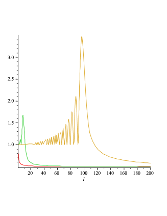
Figure 2: Plots of $|m_{n}(1,l)|,$ $|m_{n}(10,l)|,$ $|m_{n}(100,l)|.$

For fixed $l$ the solutions of $m_{n}(k,l)=0$ have $\operatorname{Im}k<0.$ If $l$ is fixed then the imaginary parts of the roots of $m_{n}(k,l)=0,$ decrease in proportion to minus the log of the real part,

$$\operatorname{Im}k\propto-\frac{1}{2}\log\operatorname{Re}k.$$ (160)

The first 50 zeros of $m_{n}(k,1),$ $m_{n}(k,5),$ and $m_{n}(k,7)$ are shown in Figure 3.

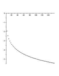
(a) Zeros of $m_{n}(k,1).$

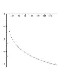
(b) Zeros of $m_{n}(k,5).$

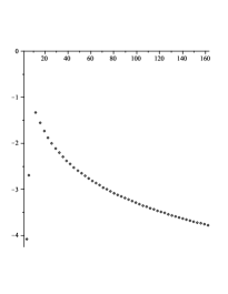
(c) Zeros of $m_{n}(k,7).$

Figure 3: Graphs of the first 50 zeros of the multipliers $m_{n}(k,l)$ for $l=1,5,7.$

Using the three term recurrence relations for spherical Bessel functions, $\{z_{l}\},$ we easily obtain the functional equation:

$$z_{l}(-\bar{k})=(-1)^{l}\overline{z_{l}(k)};$$ (161)

using this identity and (152) it is not difficult to show that

$$m_{n}(-\bar{k},l)=\overline{m_{n}(k,l)}.$$ (162)

The function $h^{(1)}_{l}$ can be factored as

$$h^{(1)}_{l}(k)=p_{l}(k)\frac{e^{ik}}{k^{l+1}},$$ (163)

where $p_{l}$ is a polynomial of degree $l.$ Thus the multiplier takes the form

$$\begin{split}m_{n}(k,l)&=p_{l}(k)e^{ik}\left(\frac{(i+k)j_{l}(k)+ikj_{l}^{\prime}(k)}{k^{l}}\right)\\ &=p_{l}(k)e^{ik}\left(\frac{(k-il)j_{l}(k)+ikj_{l-1}(k)}{k^{l}}\right)\end{split}$$ (164)

It is easy to see that the numerator has a zero of order $l$ at $k=0,$ and therefore the quotient is regular and non-vanishing there. The polynomial contributes $l$ roots; the symmetry, (162), shows that, when $l$ is odd, one root lies on the negative imaginary axis. A plot showing the roots with smallest imaginary part, and positive real part is shown in Figure 4.

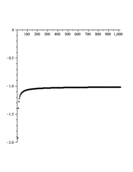
Figure 4: The solutions of $m_{n}(k,l)=0$ with smallest modulus, and positive real part, for $l=1$ to $1000.$ The real part increases monotonely with $l.$

Remark 15.

Theorem 10 shows that the frequencies $k,$ with $\operatorname{Im}k\geq 0$, for which equation (33) has a non-trivial null-space coincides with the eigenvalues of the interior boundary value problem for Maxwell’s equations defined by

$$\boldsymbol{\xi}_{-}\upharpoonright_{\Gamma}=i_{\boldsymbol{n}}\boldsymbol{\eta}_{-}\upharpoonright_{\Gamma}.$$ (165)

Of course there are no eigenvalues, or resonances with $\operatorname{Im}k\geq 0.$ Calculations like those above, though simpler, show that the boundary condition holds for the vector spherical harmonics of order $l$ provided:

$$(i+k)j_{l}(k)+ikj_{l}^{\prime}(k)=0\text{ with }k\neq 0.$$ (166)

From (164), we see that the left hand side of (166) is a factor of $m_{n}(k,l).$ Thus the eigenvalues of the interior problem are a subset of the resonances of the exterior problem. These eigenvalues are the “non-physical” interior resonances connected with our representation (83) of $\boldsymbol{\xi}$ and $\boldsymbol{\eta}$ in terms of potentials. They are familiar from the EFIE and MFIE representation, but shifted to the lower half plane, where they do no serious harm. The roots of $h^{(1)}_{l}(k)$ are known to be related to scattering resonances for scattering off of a conducting sphere.

9 The Hybrid Equations on the Unit Sphere

To find the precise form of the hybrid operator, $\mathcal{Q}^{+}(k),$ on the unit sphere, we only need to work out $-G_{0}d^{*}_{S^{2}_{1}}\star_{2}\mathcal{T}^{+}_{\boldsymbol{\xi}}(k).$ The normal equation is given by (153). As in the previous section, we represent $\boldsymbol{\xi}$ and $\boldsymbol{\eta}$ in terms of the potentials $\boldsymbol{\alpha},\boldsymbol{\alpha}_{m},\phi,$ and $\Phi_{m},$ with $\boldsymbol{j}=\boldsymbol{j}_{R}(r,q,k)$ a 1-form on $S^{2}_{1}$ and $\boldsymbol{m}=\star_{2}\boldsymbol{j}.$ The generalized Debye sources $r,q$ satisfy (145) and (146). The $\boldsymbol{\xi}$-field is given, in terms of the potentials by

$$\boldsymbol{\xi}=[ikG_{k}\boldsymbol{j}\cdot d\boldsymbol{x}-dG_{k}r-\star_{3}dG_{k}\star_{2}\boldsymbol{j}\cdot d\boldsymbol{x}].$$ (167)

Using the expressions for $r$ and $\boldsymbol{j}$ in terms of spherical, resp. vector spherical harmonics, we see that the tangential components of $\boldsymbol{\xi}_{+}$ modulo $\ker d_{S^{2}_{1}}^{*},$ are given by

$$\begin{split}&\boldsymbol{\xi}_{+t}\text{mod}\ker d_{S^{2}_{1}}^{*}=\\ &\sum_{l,m}d_{S^{2}_{1}}Y_{l}^{m}\Bigg{[}\left(\frac{-k^{2}\alpha_{lm}}{2l+1}\right)[(l+1)j_{l-1}(k)h^{(1)}_{l-1}(k)+lj_{l+1}h^{(1)}_{l+1}(k)]\\ -&ika_{lm}j_{l}(k)h^{(1)}_{l}(k)+ik\alpha_{lm}j_{l}(k)[h^{(1)}_{l}(k)+k\partial_{k}h^{(1)}_{l}(k)]\Bigg{]}\end{split}$$ (168)

Using (146) and the identity,

$$G_{0}d_{S^{2}_{1}}^{*}[d_{S^{2}_{1}}Y_{l}^{m}]=\frac{l(l+1)}{2l+1}Y^{l}_{m},$$ (169)

we easily obtain that

$$\begin{split}G_{0}d^{*}_{S^{2}_{1}}&\mathcal{T}^{+}_{\boldsymbol{\xi}}(k)\left(\begin{matrix}r\\ q\end{matrix}\right)=\sum_{l,m}\left(\frac{a_{lm}Y_{l}^{m}}{2l+1}\right)\times\\ &\Bigg{[}-ikl(l+1)j_{l}(k)h^{(1)}_{l}(k)+k^{2}j_{l}(k)[h^{(1)}_{l}(k)+k\partial_{k}h^{(1)}_{l}(k)]\\ &+\frac{ik^{3}[(l+1)j_{l-1}(k)h^{(1)}_{l-1}(k)+lj_{l+1}h^{(1)}_{l+1}(k)]}{2l+1}\Bigg{]}.\end{split}$$ (170)

As with the system of normal equations, the hybrid equations are decoupled, providing one equation for the coefficients of $r$ and one for the coefficients of $q.$ The only term on the right hand side of (170) that is not $O(l^{-1})$ is

$$\frac{-ikl(l+1)j_{l}(k)h^{(1)}_{l}(k)}{2l+1}=\frac{-1}{4}+O(l^{-1}),$$ (171)

in agreement with (48). We use the identity

$$\partial_{k}(kh^{(1)}_{l}(k))=kh^{(1)}_{l-1}(k)-lh^{(1)}_{l}(k)$$ (172)

to remove the derivative from (170), and define the multiplier for the tangential equation:

$$\begin{split}m_{t}(k,l)=&\left(\frac{-k}{2l+1}\right)\Bigg{[}il(l+1)j_{l}(k)h^{(1)}_{l}(k)-kj_{l}(k)[kh^{(1)}_{l-1}(k)-lh^{(1)}_{l}(k)]\\ &-\frac{ik^{2}[(l+1)j_{l-1}(k)h^{(1)}_{l-1}(k)+lj_{l+1}(k)h^{(1)}_{l+1}(k)]}{2l+1}\Bigg{]}.\end{split}$$ (173)

This multiplier behaves much like the multiplier $m_{n}(k,l)$ found for the normal equations. For fixed $l$ its roots, as a function of $k,$ lie in the lower half plane. The plots in Figure 5 show contours of $\log|m_{t}(k,l)|$ for $l=1,10,20.$ The $x$-axis is shown as a black horizontal line. They clearly show that the zeros lie in the lower half plane, and indicate the moderate behavior of the multiplier in the upper half plane. The plots in Figure 6 show the $|m_{t}(k,l)|$ for $l$ between $1$ and $20,$ and $20$ and $200,$ respectively, for and $k=1,10$ and $100.$ It should be recalled that there is a certain amount of arbitrariness in the definition of this multiplier, resulting from the arbitrariness in the choice of preconditioner, $G_{0}d_{S^{2}_{1}}^{*}$ in the present instance.

If the incoming tangential data are given by

$$\boldsymbol{\xi}_{t}^{\operatorname{in}}=\sum_{l,m}\left[p_{lm}\frac{d_{S^{2}_{1}}Y_{l}^{m}}{\sqrt{l(l+1)}}+q_{lm}\frac{\star_{2}d_{S^{2}_{1}}Y_{l}^{m}}{\sqrt{l(l+1)}}\right],$$ (174)

(here we used the normalized basis elements) then

$$\begin{split}i_{\boldsymbol{n}}\star_{3}\boldsymbol{\eta}^{\operatorname{in}}=\frac{\star_{2}d_{S^{2}_{1}}\boldsymbol{\xi}_{t}^{\operatorname{in}}}{ik}=\sum_{l,m}q_{lm}\frac{\star_{2}d_{S^{2}_{1}}\star_{2}d_{S^{2}_{1}}Y_{l}^{m}}{ik\sqrt{l(l+1)}}\\ =-\frac{1}{ik}\sum_{l,m}\sqrt{l(l+1)}q_{lm}Y_{l}^{m}.\end{split}$$ (175)

To find the tangential data for the hybrid system we apply $G_{0}d_{S^{2}_{1}}^{*}$ to $\boldsymbol{\xi}_{t}^{\operatorname{in}},$ obtaining:

$$G_{0}d_{S^{2}_{1}}^{*}\boldsymbol{\xi}_{t}^{\operatorname{in}}=\sum_{l,m}\frac{\sqrt{l(l+1)}}{2l+1}p_{lm}Y_{l}^{m}.$$ (176)

For the unit sphere, the hybrid equations are therefore:

$$\begin{split}m_{n}(k,l)b_{lm}&=\frac{\sqrt{l(l+1)}q_{lm}}{ik}\\ m_{t}(k,l)a_{lm}&=\frac{\sqrt{l(l+1)}}{2l+1}p_{lm}.\end{split}$$ (177)

These equations display a mild sort of low frequency breakdown, in that the coefficients of the normal data, $\{\sqrt{l(l+1)}q_{lm}\},$ must be uniformly $O(\omega)$ in order for this system of equations to be stable. Of course the incoming data $(\boldsymbol{\xi}_{+}^{\operatorname{in}},\boldsymbol{\eta}_{+}^{\operatorname{in}})$ is assumed to be a solution of the THME([)$k$], so these estimates should automatically hold. Indeed if $\boldsymbol{\eta}_{+}^{\operatorname{in}}$ is given, then there is no need to differentiate $\boldsymbol{\xi}_{+}^{\operatorname{in}},$ and divide by $k$ to find the data for the normal equation.

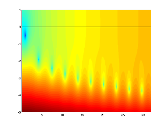
(a) Contour plot of of $\log|m_{t}(k,1)|.$

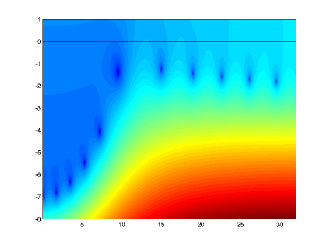
(b) Contour plot of of $\log|m_{t}(k,10)|.$

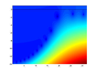
(c) Contour plot of of $\log|m_{t}(k,25)|.$

Figure 5: Plots of $\log|m_{t}(k,1)|,$ $\log|m_{t}(k,10)|,$ $\log|m_{t}(k,25)|.$ The black horizontal line indicates the $x$-axis. The zeros are located near the deep blue dots.

The use of $G_{0}$ in the preconditioner also leads to growth in the multiplier $m_{t}(k,l)$ are $k$ increases for fixed $l$. Figure 6(c) show $|m_{t}(k,1)|,|m_{t}(k,10)|,$ and $|m_{t}(k,20)|,$ for real $k\in[0,100].$ In the interval $0<k<l$ these functions oscillate around a small non-zero value. When $k$ exceeds $l$ these functions show linear growth. Replacing $G_{0},$ with something like $G_{i|k|}$ should fix this problem.

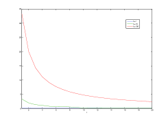
(a) Small $l$

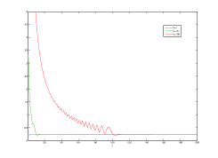
(b) Large $l$

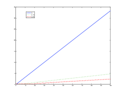
(c) Fixed $l$

Figure 6: Plots of $|m_{t}(k,1)|,$ for a large range of $l$ and $k=1,10,100,$ and fixed $l=1,10,20$ with $k\in[0,100].$

10 Conclusions

In this paper, we have developed a new representation for solutions of the time harmonic Maxwell equations, exterior to closed surfaces, based on two scalar densities. In the zero frequency limit, these densities are uncoupled and correspond to electric and magnetic charge. At non-zero frequency, however, they do not correspond directly to physical variables. They are simply used to construct electric and magnetic currents, after which the classical scalar and vector potentials and anti-potentials are employed (in the usual Lorenz gauge). Because of the close connection to the Lorenz-Debye-Mie formalism when the analysis is restricted to the unit sphere, we refer to our unknowns as generalized Debye sources. The natural boundary data for our unknowns are the normal components of the electric and magnetic field and we have provided a detailed uniqueness theory for this boundary value problem for boundary surfaces of arbitrary genus (Theorems 4, 5, 9). In the course of this analysis, we have given a new proof of the existence (in the non-simply connected case) of families of nontrivial solutions with zero boundary data, which we refer to as $k$-Neumann fields. They generalize, to non-zero wave numbers, the classical harmonic Neumann fields (Theorem 11).

We have also introduced a new Fredholm integral equation of the second kind for scattering from a perfect electrical conductor and have shown that it is invertible (in the simply connected case) for all wave numbers $k$ in the closed upper half plane. There is a natural extension of the approach to the case of a dielectric interface, which will be reported at a later date.

The work begun here gives rise to a new set of analytic and computational issues. In order to use the Debye sources as unknowns, one needs an efficient and accurate method for inverting the surface Laplacian. For surfaces $\Gamma$ of genus $g>0$, we also need to be able to efficiently construct a basis for the harmonic forms $\mathcal{H}^{1}(\Gamma).$ Finally, additional work is required to extend our approach to open surfaces (see, for example, [14]). These arise as common and important idealizations in the analysis of thin plates, cylindrical conductors and metallized surface patches in radar, medical imaging, chip design and remote sensing applications.

Appendix

Appendix A Exterior Forms, Maxwell Equations and Vector Spherical Harmonics

In the traditional approach to electricity and magnetism Maxwell’s equations are expressed in terms of relationships between four vector fields $\boldsymbol{E},\boldsymbol{D}$ and $\boldsymbol{B},\boldsymbol{H}$ defined on $\mathbb{R}^{3}\times\mathbb{R}:$

$$\begin{split}\frac{\partial\boldsymbol{D}}{\partial t}=c\nabla\times\boldsymbol{H}-4\pi\boldsymbol{J}&\quad\frac{\partial\boldsymbol{B}}{\partial t}=-c\nabla\times\boldsymbol{E}\\ \nabla\cdot\boldsymbol{D}=4\pi\rho&\quad\nabla\cdot\boldsymbol{B}=0;\end{split}$$ (178)

$c$ is the speed of light. Here $\boldsymbol{J}$ is the current density and $\rho$ is the charge density, they satisfy the conservation of charge:

$$\frac{\partial\rho}{\partial t}=-\nabla\cdot\boldsymbol{J}.$$ (179)

The differential symmetries of this system of equations are rooted in the exactness of the sequence:

$${\mathcal{C}}^{\infty}(U)\overset{\nabla}{\longrightarrow}{\mathcal{C}}^{\infty}(U;T\mathbb{R}^{3})\overset{\nabla\times}{\longrightarrow}{\mathcal{C}}^{\infty}(U;T\mathbb{R}^{3})\overset{\nabla\cdot}{\longrightarrow}{\mathcal{C}}^{\infty}(U),$$ (180)

here $U\subset\mathbb{R}^{3}$ is an open set, and ${\mathcal{C}}^{\infty}(U;T\mathbb{R}^{3})$ are the smooth vector fields defined in $U:$

$${\mathcal{C}}^{\infty}(U;T\mathbb{R}^{3})=\{a_{1}(x)\partial_{x_{1}}+a_{2}(x)\partial_{x_{2}}+a_{3}(x)\partial_{x_{3}}:\>a_{1},a_{2},a_{3}\in{\mathcal{C}}^{\infty}(U)\}.$$ (181)

The exactness of the sequence is equivalent to the classical identities $\nabla\times\nabla=0,$ and $\nabla\cdot\nabla\times=0.$

While this representation is traditional, physically and geometrically it makes more sense to regard Maxwell’s equations as a relationship amongst differential, or exterior forms. In the second part of this paper we usually work with the fields $\boldsymbol{E}$ and $\boldsymbol{H}.$ It turns out to be convenient to use a 1-form to represent $\boldsymbol{E}$ and a 2-form to represent $\boldsymbol{H}.$ We use the correspondences

$$\begin{split}\boldsymbol{H}=h_{1}\partial_{x_{1}}+h_{2}\partial_{x_{2}}+h_{3}\partial_{x_{3}}&\leftrightarrow h_{1}dx_{2}\wedge dx_{3}+h_{2}dx_{3}\wedge dx_{1}+h_{3}dx_{1}\wedge dx_{2}=\boldsymbol{\eta}\\ \boldsymbol{E}=e_{1}\partial_{x_{1}}+e_{2}\partial_{x_{2}}+e_{3}\partial_{x_{3}}&\leftrightarrow e_{1}dx_{1}+e_{2}dx_{2}+e_{3}dx_{3}=\boldsymbol{\xi}\end{split}$$ (182)

Under this correspondence $\boldsymbol{\xi}$ is the metric dual of $\boldsymbol{E}$ and $\star\boldsymbol{\eta}$ ($\star$ is the Hodge star-operator defined by the metric on $\mathbb{R}^{3}$) is the metric dual of $\boldsymbol{H}.$

It is natural to think of the electric field as a 1-form, for the electric potential difference is then obtained by integrating this 1-form:

$$\phi_{P}-\phi_{Q}=\int\limits_{\gamma}\boldsymbol{\xi},$$ (183)

with $\gamma$ a path from $P$ to $Q.$ Similarly, it is reasonable to think of the magnetic field as a 2-form, for the flux of $\boldsymbol{H}$ through a surface $\Sigma$ is then obtained by integrating:

$$\text{Flux of $\boldsymbol{H}$ through }\Sigma=\int\limits_{\Sigma}\boldsymbol{\eta}.$$ (184)

While these are the most basic measurements associated to electric and magnetic fields, there are times when it is natural to integrate the $\boldsymbol{E}$-field over a surface, or the $\boldsymbol{H}$-field over a curve. This is done, in the form language, by using the Hodge-star and interior product operations, $\star,i_{\boldsymbol{v}},$ introduced below. A detailed exposition of this approach to Maxwell’s equations can be found in [3].

For the sake of completeness we recall the definition of $d$ on forms defined on $\mathbb{R}^{3}:$

$$\begin{split}&0\text{-forms }\Lambda^{0}\mathbb{R}^{3}:\quad da=\partial_{x_{1}}adx_{1}+\partial_{x_{2}}adx_{2}+\partial_{x_{3}}adx_{3}\\ &1\text{-forms }\Lambda^{1}\mathbb{R}^{3}:\quad d(a_{1}dx_{1}+a_{2}dx_{2}+a_{3}dx_{3})=(\partial_{x_{1}}a_{2}-\partial_{x_{1}}a_{1})dx_{1}\wedge dx_{2}\\ &\phantom{ll}+(\partial_{x_{3}}a_{1}-\partial_{x_{1}}a_{3})dx_{3}\wedge dx_{1}+(\partial_{x_{2}}a_{3}-\partial_{x_{3}}a_{2})dx_{2}\wedge dx_{3}\\ &2\text{-forms }\Lambda^{2}\mathbb{R}^{3}:\quad d(a_{1}dx_{1}\wedge dx_{2}+a_{2}dx_{3}\wedge dx_{1}+a_{3}dx_{2}\wedge dx_{3})=\\ &\phantom{\text{ll}}(\partial_{x_{1}}a_{1}+\partial_{x_{2}}a_{2}+\partial_{x_{3}}a_{3})dx_{1}\wedge dx_{2}\wedge dx_{3}\\ &3\text{-forms }\Lambda^{3}\mathbb{R}^{3}:\quad d(adx_{1}\wedge dx_{2}\wedge dx_{3})=0.\end{split}$$ (185)

The sequence (180) becomes:

$${\mathcal{C}}^{\infty}(U)\overset{d}{\longrightarrow}{\mathcal{C}}^{\infty}(U;\Lambda^{1}\mathbb{R}^{3})\overset{d}{\longrightarrow}{\mathcal{C}}^{\infty}(U;\Lambda^{2}\mathbb{R}^{3})\overset{d}{\longrightarrow}{\mathcal{C}}^{\infty}(U;\Lambda^{3}\mathbb{R}^{3}).$$ (186)

All of the classical differential relations are simply $d^{2}=0.$

A.1 Exterior forms on a manifold

Generally we can define the smooth exterior $p$-forms on an $n$-dimensional manifold $M,$ ${\mathcal{C}}^{\infty}(M;\Lambda^{p}T^{*}M),$ as sections of the vector bundle $\Lambda^{p}T^{*}M.$ The exterior derivative is a canonical map

$$d:{\mathcal{C}}^{\infty}(M;\Lambda^{p}T^{*}M)\to{\mathcal{C}}^{\infty}(M;\Lambda^{p+1}T^{*}M).$$ (187)

If $(x_{1},\dots,x_{n})$ are local coordinates, then a $p$-form can be expressed as

$$\boldsymbol{\alpha}=\sum_{I\in\mathcal{I}_{p}}a_{I}(x)dx_{i_{1}}\wedge\cdots\wedge dx_{i_{p}},\quad a_{I}\in{\mathcal{C}}^{\infty}.$$ (188)

Here $\mathcal{I}_{p}$ is the set of increasing $p$-multi-indices $1\leq i_{1}<\cdots<i_{p}\leq n.$ In these local coordinates, the exterior derivative of a function $f(x)$ is defined to be

$$df=\sum_{j=1}^{n}\partial_{x_{j}}f(x)dx_{j},$$ (189)

and of a $p$-form

$$d\boldsymbol{\alpha}=\sum_{I\in\mathcal{L}_{p}}da_{I}(x)\wedge dx_{i_{1}}\wedge\cdots\wedge dx_{i_{p}}.$$ (190)

The remarkable fact is that this is invariantly defined; though it is really nothing more than the chain rule. The fact that mixed partial derivatives commute easily applies to show that $d^{2}=0.$ If $\boldsymbol{\alpha}$ and $\boldsymbol{\beta}$ are forms, then we have the Leibniz Formula:

$$d(\boldsymbol{\alpha}\wedge\boldsymbol{\beta})=(d\boldsymbol{\alpha})\wedge\boldsymbol{\beta}+(-1)^{\deg\boldsymbol{\alpha}}\boldsymbol{\alpha}\wedge d\boldsymbol{\beta}.$$ (191)

If $\boldsymbol{\alpha}$ is a $k$-form defined in an open subset, $U$ of $M$ then we can integrate it over any smooth, oriented compact submanifold $\Sigma^{k}\subset\!\subset U,$ of dimension $k,$ with or without boundary. We denote this pairing by

$$\left<\boldsymbol{\alpha},[\Sigma]\right>=\int\limits_{\Sigma}\boldsymbol{\alpha}.$$ (192)

If $\boldsymbol{\alpha}$ is an exact form, that is, $\boldsymbol{\alpha}=d\boldsymbol{\beta},$ and $\Sigma$ is a smooth, oriented submanifold with or without boundary, then Stokes’ theorem states that

$$\int\limits_{\Sigma}d\boldsymbol{\beta}=\int\limits_{\partial\Sigma}\boldsymbol{\beta}.$$ (193)

The boundary must be given the induced orientation. Note, in particular, that if $\partial\Sigma=\emptyset,$ then the integral of $d\boldsymbol{\beta}$ over $\Sigma$ vanishes.

There is a second natural operation on exterior forms that satisfies a Leibniz formula. If $\boldsymbol{v}$ is a vector field, then the interior product of $\boldsymbol{v}$ with a $k$-form, $\omega,$ is a $(k-1)$-form, $i_{\boldsymbol{v}}\omega,$ defined by:

$$i_{\boldsymbol{v}}\omega(\boldsymbol{v}_{2},\dots,\boldsymbol{v}_{k})\overset{d}{=}\omega(\boldsymbol{v},\boldsymbol{v}_{2},\dots,\boldsymbol{v}_{k}).$$ (194)

If $\omega$ and $\eta$ are exterior forms, then

$$i_{\boldsymbol{v}}[\omega\wedge\eta]=[i_{\boldsymbol{v}}\omega]\wedge\eta+(-1)^{\deg\omega}\omega\wedge[i_{\boldsymbol{v}}\eta].$$ (195)

Using forms simplifies calculations considerably because forms can be automatically integrated over submanifolds of the “correct” dimension, keep track of orientation, and all the differential relationships follow from the fact that $d^{2}=0.$ Moreover, Stokes’ theorem subsumes all the classical integration by parts formulæ is one simple package.

A.2 Hodge star-operator

To write the Maxwell equations we need one further operation, called the Hodge star-operator. This operation can be defined on an oriented Riemannian manifold. Suppose that $\omega_{1},\dots,\omega_{n}$ is an local orthonormal basis of one forms, and

$$dV=\omega_{1}\wedge\cdots\wedge\omega_{n},$$ (196)

defines the orientation. If $1\leq i_{1}<\cdots<i_{p}\leq n,$ and $j_{1}<\cdots<j_{n-p}$ are complementary indices, then we define

$$\star[\omega_{i_{1}}\wedge\cdots\wedge\omega_{i_{p}}]=(-1)^{\epsilon}\omega_{j_{1}}\wedge\cdots\wedge\omega_{j_{n-p}},$$ (197)

with $\epsilon=0$ or $1,$ chosen so that

$$\omega_{i_{1}}\wedge\cdots\wedge\omega_{i_{p}}\wedge\star[\omega_{i_{1}}\wedge\cdots\wedge\omega_{i_{p}}]=dV.$$ (198)

For example, the Hodge operator is defined on the standard orthonormal basis of exterior forms for $\mathbb{R}^{3}$ by setting:

$$\begin{split}\star 1&=dx_{1}\wedge dx_{2}\wedge dx_{3}\\ \star dx_{1}=dx_{2}\wedge dx_{3}\quad\star dx_{2}&=dx_{3}\wedge dx_{1}\quad\star dx_{3}=dx_{1}\wedge dx_{2}\\ \star dx_{1}\wedge dx_{2}=dx_{3}\quad\star dx_{3}\wedge dx_{1}&=dx_{2}\quad\star dx_{2}\wedge dx_{3}=dx_{1}\\ \star dx_{1}\wedge dx_{2}\wedge dx_{3}&=1\end{split}$$ (199)

From these formulæ it is clear that, in 3-dimensions, $\star^{2}=I.$ Notice that applying the $\star$-operator exchanges the two correspondences between vector fields and forms in (182).

The star-operator is simply related to the metric: If $\boldsymbol{\alpha},\boldsymbol{\beta}$ are real $p$-forms, then

$$[\boldsymbol{\alpha}\wedge\star\boldsymbol{\beta}]_{x}=(\boldsymbol{\alpha},\boldsymbol{\beta})_{x}dV_{x},$$ (200)

where $(\cdot,\cdot)$ is the (real) inner product defined by the metric on $p$-forms. Generally,

$$\star^{2}=(-1)^{p(n-p)},$$ (201)

on $p$-forms defined on an $n$-dimensional manifold. Using this observation and (200) we easily show that $\star$ is a pointwise isometry:

$$(\boldsymbol{\alpha},\boldsymbol{\beta})_{x}=(\star\boldsymbol{\alpha},\star\boldsymbol{\beta})_{x}$$ (202)

A fundamental role of the Hodge $\star$-operator is to define a Hilbert space inner product on forms. If $\boldsymbol{\alpha}$ and $\boldsymbol{\beta}$ are (possibly complex) forms of the same degree defined in $U,$ then $\boldsymbol{\alpha}\wedge\star\overline{\boldsymbol{\beta}}$ is a $n$-form, which can therefore be integrated:

$$\begin{split}\langle\boldsymbol{\alpha},\boldsymbol{\beta}\rangle&=\int\limits_{U}\boldsymbol{\alpha}\wedge\star\overline{\boldsymbol{\beta}}.\\ &=\int\limits_{U}(\boldsymbol{\alpha},\boldsymbol{\beta})_{x}dV(x).\end{split}$$ (203)

We assume that $(\cdot,\cdot)$ is extended to define an Hermitian inner product on complex valued forms. The extended metric continues to satisfy (202).

A.3 Adjoints, Integration-by-parts and the Hodge Theorem

On an $n$-dimensional manifold the expression for the formal adjoint, with respect to the pairing in (203), of the $d$-operator, acting on a $p$-form $\boldsymbol{\beta},$ is:

$$d^{*}\boldsymbol{\beta}=\begin{cases}-\star d\star\boldsymbol{\beta}&\text{ if }n\text{ is even}\\ (-1)^{p}\star d\star\boldsymbol{\beta}&\text{ if }n\text{ is odd.}\end{cases}$$ (204)

Let $G$ be a bounded domain with a smooth boundary. Let $r$ be a function that is negative in $G$ and vanishes on $bG.$ Suppose moreover that $(dr,dr)_{x}\equiv 1$ for $x\in bG,$ and $\boldsymbol{n}$ is the outward pointing unit normal along $bG.$ The basic integration by parts formulæ for $d$ and $d^{*}$ can be expressed in terms of this inner product by

$$\begin{split}\langle d\boldsymbol{\alpha},\boldsymbol{\beta}\rangle_{G}&=\int\limits_{bG}(dr\wedge\boldsymbol{\alpha},\boldsymbol{\beta})_{x}dS(x)+\langle\boldsymbol{\alpha},d^{*}\boldsymbol{\beta}\rangle_{G}\\ \langle d^{*}\boldsymbol{\alpha},\boldsymbol{\beta}\rangle_{G}&=-\int\limits_{bG}(i_{\boldsymbol{n}}\boldsymbol{\alpha},\boldsymbol{\beta})_{x}dS(x)+\langle\boldsymbol{\alpha},d\boldsymbol{\beta}\rangle_{G}.\end{split}$$ (205)

Here we use $dS$ to denote surface measure on $bG.$ It is important to recall that, with respect to the pointwise inner product,

$$(dr\wedge\boldsymbol{\alpha},\boldsymbol{\beta})_{x}=(\boldsymbol{\alpha},i_{\boldsymbol{n}}\boldsymbol{\beta})_{x}.$$ (206)

The (positive) Laplace operator, acting on any form degree is given by formula

$$dd^{*}+d^{*}d.$$ (207)

In $\boldsymbol{R}^{3}$ this would give $-(\partial^{2}_{x_{1}}+\partial^{2}_{x_{2}}+\partial^{2}_{x_{3}}).$ To avoid confusion with standard usage in E&M, we use $\Delta$ to denote the negative operator $-(dd^{*}+d^{*}d).$ If $M$ is a compact manifold without boundary, then the de Rham cohomology groups are defined, for $0\leq k\leq\dim M,$ as

$$H_{\operatorname{dR}}^{k}(M)\\ =\operatorname{ker}\{d:{\mathcal{C}}^{\infty}(M;\Lambda^{k}T^{*}M)\to{\mathcal{C}}^{\infty}(M;\Lambda^{k+1}T^{*}M)\}/d{\mathcal{C}}^{\infty}(M;\Lambda^{k-1}T^{*}M).$$ (208)

It is a classical theorem that these abelian group are topological invariants, see [29]. We let $\mathcal{H}^{k}(M)$ denote the nullspace of the Laplacian acting on ${\mathcal{C}}^{\infty}(M;\Lambda^{k}T^{*}M).$ Stokes’ theorem shows that

$$\langle\Delta\omega,\omega\rangle=\langle d\omega,d\omega\rangle+\langle d^{*}\omega,d^{*}\omega\rangle.$$ (209)

Thus $\mathcal{H}^{k}(M)\simeq\operatorname{ker}d\cap\operatorname{ker}d^{*}.$ The Hodge theorem states that

Theorem 15 (Hodge).

If $(M,g)$ is a compact Riemannian manifold, without boundary, then, for each $0\leq k\leq\dim M,$

$$\mathcal{H}^{k}(M)\simeq H^{k}_{\operatorname{dR}}(M).$$ (210)

and, as an $L^{2}$-orthogonal direct sum, we have:

$${\mathcal{C}}^{\infty}(M;\Lambda^{k}T^{*}M)=d{\mathcal{C}}^{\infty}(M;\Lambda^{k-1}T^{*}M)\oplus d^{*}{\mathcal{C}}^{\infty}(M;\Lambda^{k+1}T^{*}M)\oplus\mathcal{H}^{k}(M).$$ (211)

As $\Delta$ is an elliptic operator, the Hodge theorem has the following very useful corollary:

Corollary 6.

If $(M,g)$ is a compact Riemannian manifold, without boundary, then for each $0\leq k\leq\dim M,$ the $\dim H^{k}_{\operatorname{dR}}(M)$ is finite.

A.4 Maxwell’s Equations in terms of exterior forms

With these preliminaries we can state the correspondences between the differential operators, $\nabla,\nabla\times,$ and $\nabla\cdot$ and the corresponding objects acting on forms. For a scalar function $\phi,$ $\nabla\phi$ corresponds to $d\phi.$ An elementary calculation shows that if $\boldsymbol{E}\leftrightarrow\boldsymbol{\xi},$ a 1-form, then $\nabla\times\boldsymbol{E}\leftrightarrow d\boldsymbol{\xi},$ and $\nabla\cdot\boldsymbol{E}\leftrightarrow d^{*}\boldsymbol{\xi}.$ Moreover with $\boldsymbol{H}\leftrightarrow\boldsymbol{\eta},$ a 2-form, we have $\nabla\times\boldsymbol{H}\leftrightarrow d^{*}\boldsymbol{\eta},$ and $\nabla\cdot\boldsymbol{H}\leftrightarrow d\boldsymbol{\eta}.$ The operator $d^{*}$ also acts on $3$-forms.

If we let $\boldsymbol{E}\leftrightarrow\boldsymbol{\xi},$ $\boldsymbol{H}\leftrightarrow\boldsymbol{\eta},$ and $\boldsymbol{J}\leftrightarrow\boldsymbol{j}$ (a 1-form) as in (182), then Maxwell’s equations in a vacuum become:

$$\begin{split}\frac{\partial\boldsymbol{\xi}}{\partial t}=cd^{*}\boldsymbol{\eta}-4\pi\boldsymbol{j}&\quad\frac{\partial\boldsymbol{\eta}}{\partial t}=-cd\boldsymbol{\xi}\\ d^{*}\boldsymbol{\xi}=4\pi\rho\quad d\boldsymbol{\eta}&=0\quad\frac{\partial\rho}{\partial t}=-d^{*}\boldsymbol{j}.\end{split}$$ (212)

If $\boldsymbol{\xi}$ and $\boldsymbol{\eta}$ are time harmonic with time dependence $e^{-it\omega},$ then in the absence of sources, we easily derive the Helmholtz equations:

$$c^{2}\Delta\boldsymbol{\xi}+\omega^{2}\boldsymbol{\xi}=0\quad c^{2}\Delta\boldsymbol{\eta}+\omega^{2}\boldsymbol{\eta}=0.$$ (213)

We let $D\subset\mathbb{R}^{3}$ denote a bounded set with smooth boundary and let

$$\Omega=\mathbb{R}^{3}\setminus\overline{D}\quad\Gamma=bD.$$ (214)

In this paper $D$ is usually taken to be a perfect conductor, lying in a bounded domain with smooth boundary, and $\Omega$ a dielectric. We assume that $\epsilon$ is the electrical permittivity, $\mu$ is the magnetic permeabilty and $\sigma$ the electrical conductivity of $\Omega.$ As above, we identify the $\boldsymbol{E}$-field with a 1-form, $\boldsymbol{\Xi}:$

$$e_{1}\partial_{x_{1}}+e_{2}\partial_{x_{2}}+e_{3}\partial_{x_{3}}=\boldsymbol{E}\leftrightarrow\boldsymbol{\Xi}=e_{1}dx_{1}+e_{2}dx_{2}+e_{3}dx_{3},$$ (215)

and $\boldsymbol{H}$ with a 2-form, $\boldsymbol{N}:$

$$h_{1}\partial_{x_{1}}+h_{2}\partial_{x_{2}}+h_{3}\partial{x_{3}}=\boldsymbol{H}\leftrightarrow\boldsymbol{N}=h_{1}dx_{2}\wedge dx_{3}+h_{2}dx_{3}\wedge dx_{1}+h_{3}dx_{1}\wedge dx_{2}.$$ (216)

In terms of exterior forms, we set

$$\boldsymbol{\Xi}(x,t)=\left[\frac{\omega}{\omega\epsilon+i\sigma}\right]^{\frac{1}{2}}\boldsymbol{\xi}(x)e^{-i\omega t}\quad\boldsymbol{N}(x,t)=\mu^{-\frac{1}{2}}\boldsymbol{\eta}(x)e^{-i\omega t};$$ (217)

the time harmonic Maxwell equations become:

$$\begin{split}&d\boldsymbol{\xi}=ik\boldsymbol{\eta}\quad d^{*}\boldsymbol{\xi}=0\\ &d^{*}\boldsymbol{\eta}=-ik\boldsymbol{\xi}\quad d\boldsymbol{\eta}=0.\end{split}$$ (218)

Here $k$ is the square root of $\mu(\epsilon\omega^{2}+i\sigma\omega),$ with non-negative imaginary part.

With this choice of correspondence between the vector and form representations, we can write the Maxwell equations in a very succinct and symmetric form:

$$(d+d^{*})(\boldsymbol{\xi}+\boldsymbol{\eta})=ik\Lambda(\boldsymbol{\xi}+\boldsymbol{\eta});$$ (219)

here $\Lambda$ is the operation defined on forms by

$$\Lambda(\boldsymbol{\alpha})=(-1)^{\deg\boldsymbol{\alpha}}\boldsymbol{\alpha}.$$ (220)

Simple calculations shows that

$$(d+d^{*})\Lambda=-\Lambda(d+d^{*})\text{ and }\Lambda^{2}=I,$$ (221)

implying that

$$(d+d^{*}-ik\Lambda)^{2}=-(\Delta+k^{2}).$$ (222)

Thus, acting on forms, the operator $\Delta+k^{2}$ has a local square root. Or, put differently, $d+d^{*}-ik\Lambda$ is an operator of Dirac-type, see [5]. Indeed, we could write the vacuum Maxwell equations in the form

$$[c(d+d^{*})+\Lambda\partial_{t}](\boldsymbol{\xi}+\boldsymbol{\eta})=4\pi c\rho,$$ (223)

noting that

$$[c(d+d^{*})+\Lambda\partial_{t}]^{2}=\partial_{t}^{2}-c^{2}\Delta.$$ (224)

A.5 Vector Spherical Harmonics

The domains defined in $\mathbb{R}^{3}$ as complements of a round sphere are very important in applications. They also provide a context where the integral equations defined in the earlier sections can be diagonalized and solved explicitly in terms of classical special functions. In this appendix we give a brief treatment of the theory of vector spherical harmonics in the exterior form representation. A classical treatment is given in sections 9.6-7 of [13]. But for the classical theory of (scalar) spherical harmonics (which can also be found in Jackson), our discussion is essentially self contained.

We begin with the relationship between the (negative) Laplace operators in $\mathbb{R}^{3}$ and on the unit sphere $S^{2}_{1}\subset\mathbb{R}^{3}.$ Recall that on any Riemannian manifold, $(X,g),$ the Laplace operator on $k$-forms is given by $\Delta^{X}_{k}=-(d^{*}d+dd^{*}),$ where $*$ is defined by $g.$ The following is simply the usual change of variables formula for spherical polar coordinates.

Proposition 5.

Let $r^{2}=x_{1}^{2}+x_{2}^{2}+x_{3}^{2},$ the scalar Laplace operator on $\mathbb{R}^{3}$ can be expressed as

$$\Delta^{\mathbb{R}^{3}}_{0}=\frac{1}{r^{2}}\partial_{r}r^{2}\partial_{r}+\frac{1}{r^{2}}\Delta^{S^{2}_{1}}_{0},\text{ where }\partial_{r}=\frac{x_{1}\partial_{x_{1}}+x_{2}\partial_{x_{2}}+x_{3}\partial_{x_{3}}}{r}.$$ (225)

We also need to relate the Laplacians on 1-forms.

Proposition 6.

Let $\boldsymbol{\alpha}$ be a 1-form on $\mathbb{R}^{3}$ such that $i_{\partial_{r}}\boldsymbol{\alpha}=0,$ then

$$\Delta_{1}^{\mathbb{R}^{3}}\boldsymbol{\alpha}=\frac{1}{r^{2}}\Delta_{1}^{S^{2}_{1}}\boldsymbol{\alpha}+L_{r}\boldsymbol{\alpha}+\frac{1}{r^{2}}\left(d_{S^{2}_{1}}^{*}\boldsymbol{\alpha}\right)dr,$$ (226)

where

$$L_{r}\boldsymbol{\alpha}=i_{r^{2}\partial_{r}}d(i_{r^{-2}\partial_{r}}d\boldsymbol{\alpha})+\frac{2}{r^{2}}\boldsymbol{\alpha}.$$ (227)

This formula follows by a calculation using a local co-frame field. If we express $\boldsymbol{\alpha}=\sum\alpha_{j}dx_{j},$ then

$$L_{r}\boldsymbol{\alpha}=\sum_{j=1}^{3}(\partial_{r}^{2}\alpha_{j})dx_{j}.$$ (228)

While (226) is a good deal more complicated than (225), it allows for a careful analysis of the eigenforms of $\Delta_{1}^{S^{2}_{1}}.$

We begin with the standard description of the eigenspaces of $\Delta_{0}^{S^{2}_{1}}.$ Let $\mathcal{E}^{0}_{l}$ denote the linear space of scalar eigenfunctions on $S^{2}_{1}$ satisfying:

$$\Delta_{0}^{S^{2}_{1}}f=-l(l+1)f.$$ (229)

These spaces are represented in terms of classical spherical harmonics by

$$\mathcal{E}^{0}_{l}=\operatorname{span}\{Y_{l}^{m}:\>m=-l,\dots,l\}$$ (230)

A basis of eigenforms of $\Delta_{2}^{S^{2}_{1}},$ with eigenvalue $l(l+1),$ is given by

$$\{\star_{2}Y_{l}^{m}=Y_{l}^{m}dA:\>m=-l\dots l\}.$$

The fact that $H^{1}(S^{2};\mathbb{R})=0$ and the Hodge theorem imply that the 1-forms on $S^{2}_{1}$ are the $L^{2}$-orthogonal direct sum

$${\mathcal{C}}^{\infty}(S^{2}_{1};\Lambda^{1})=d_{S^{2}_{1}}{\mathcal{C}}^{\infty}(S^{2}_{1};\Lambda^{0})\oplus d_{S^{2}_{1}}^{*}{\mathcal{C}}^{\infty}(S^{2}_{1};\Lambda^{2}).$$ (231)

This observation coupled with the fact that $d$ and $d^{*}$ commute with $\Delta$ imply that the eigenspaces of $\Delta_{1}^{S^{2}_{1}}$ are given, for $l\in\mathbb{N},$ by

$$\mathcal{E}^{1}_{l}=\operatorname{span}\big{[}\{d_{S^{2}_{1}}Y_{l}^{m}:\>m=-l,\dots,l\}\oplus\{\star_{2}d_{S^{2}_{1}}Y_{l}^{m}:\>m=-l,\dots,l\}\big{]},$$ (232)

with eigenvalue $-l(l+1).$ From this representation, the classical orthogonality relations are quite easy:

$$\begin{split}&\langle d_{S^{2}_{1}}Y_{l}^{m},d_{S^{2}_{1}}Y_{l^{\prime}}^{m^{\prime}}\rangle=\langle d_{S^{2}_{1}}^{*}d_{S^{2}_{1}}Y_{l}^{m},Y_{l^{\prime}}^{m^{\prime}}\rangle=\delta_{ll^{\prime}}\delta^{mm^{\prime}}l(l+1)\\ &\langle\star_{2}d_{S^{2}_{1}}Y_{l}^{m},\star_{2}d_{S^{2}_{1}}Y_{l^{\prime}}^{m^{\prime}}\rangle=\langle d_{S^{2}_{1}}Y_{l}^{m},d_{S^{2}_{1}}Y_{l^{\prime}}^{m^{\prime}}\rangle=\delta_{ll^{\prime}}\delta^{mm^{\prime}}l(l+1)\\ &\langle d_{S^{2}_{1}}Y_{l}^{m},\star_{2}d_{S^{2}_{1}}Y_{l^{\prime}}^{m^{\prime}}\rangle=\langle Y_{l}^{m},d_{S^{2}_{1}}^{2}Y_{l^{\prime}}^{m^{\prime}}\rangle=0.\end{split}$$ (233)

The second line from the fact that $\star_{2}$ is an orthogonal transformation, and the last relation follows from Stokes theorem.

The eigenforms $\star_{2}d_{S^{2}_{1}}Y_{l}^{m}$ are divergence free. If we extend them to $\mathbb{R}^{3}$ so they annihilate $\partial_{r},$ and express them in the form $\star_{2}dY_{l}^{m}=a_{1}dx_{1}+a_{2}dx_{2}+a_{3}dx_{3},$ where the coefficients are extended to be homogeneous of degree $0,$ then it follows from (226) and the equation

$$\Delta_{1}^{\mathbb{R}^{3}}(a_{1}dx_{1}+a_{2}dx_{2}+a_{3}dx_{3})=(\Delta_{0}^{\mathbb{R}^{3}}a_{1})dx_{1}+(\Delta_{0}^{\mathbb{R}^{3}}a_{2})dx_{2}+(\Delta_{0}^{\mathbb{R}^{3}}a_{3})dx_{3}$$ (234)

that is, where $r=1,$ we have

$$\Delta_{0}^{S^{2}_{1}}a_{j}=-l(l+1)a_{j}.$$ (235)

In other words the coefficients of $\star_{2}d_{S^{2}_{1}}Y_{l}^{m}$ lie in $\mathcal{E}^{0}_{l}.$ These eigenforms correspond to the classical eigenfields of the form $\{\boldsymbol{r}\times\nabla Y_{l}^{m}\}.$

The members of the other family, $\{d_{S^{2}_{1}}Y_{l}^{m}\},$ which corresponds to $\{\boldsymbol{r}\times(\boldsymbol{r}\times\nabla Y_{l}^{m})\},$ are not divergence free and their coefficients with respect to $dx_{j}$ lie in $\mathcal{E}^{0}_{l-1}\oplus\mathcal{E}^{0}_{l+1}.$ These coefficients are easily found; if we think of $Y_{l}^{m}$ as a homogeneous function of degree $0$ on $\mathbb{R}^{3},$ then $i_{\partial_{r}}d_{\mathbb{R}^{3}}Y_{l}^{m}=0,$

$$d_{S^{2}_{1}}Y_{l}^{m}=\sum_{j=1}^{3}\frac{\partial Y_{l}^{m}}{\partial x_{j}}dx_{j}\upharpoonright_{S^{2}_{1}}.$$ (236)

In order to determine the action of the Green’s function on the coefficients of these forms, we need to represent them in terms of spherical harmonics. Let $U_{l}^{m}=r^{l}Y_{l}^{m}.$ This is a homogeneous harmonic polynomial of degree $l.$ We see that

$$\frac{\partial U_{l}^{m}}{\partial x_{j}}=r^{l}\frac{\partial Y_{l}^{m}}{\partial x_{j}}+l\frac{x_{j}}{r^{2}}U_{l}^{m}.$$ (237)

We apply the Laplace operator to $x_{j}U_{l}^{m}$ to obtain

$$\Delta^{\mathbb{R}^{3}}_{0}(x_{j}U_{l}^{m})=2\frac{\partial U_{l}^{m}}{\partial x_{j}},$$ (238)

and therefore

$$x_{j}U_{l}^{m}=u_{l+}^{mj}+r^{2}u_{l-}^{mj}.$$ (239)

Here $u_{l+}^{mj},u_{l-}^{mj}$ are homogeneous harmonic polynomials of degrees $l+1$ and $l-1,$ respectively. Once again applying the Laplace operator to this relation, we see that

$$u_{l-}^{mj}=\frac{1}{2l+1}\frac{\partial U_{l}^{m}}{\partial x_{j}},$$ (240)

and therefore

$$\sum_{j=1}^{3}u_{l+}^{mj}dx_{j}=U_{l}^{m}rdr-\frac{r^{2}}{2l+1}dU_{l}^{m}.$$ (241)

Using the homogeneity we also see that

$$\sum_{j=1}^{3}x_{j}u_{l+}^{mj}=\frac{l+1}{2l+1}r^{2}U_{l}^{m}.$$ (242)

Restricting to $r=1,$ gives

$$\frac{\partial Y_{l}^{m}}{\partial x_{j}}\upharpoonright_{r=1}=\frac{l+1}{2l+1}\frac{\partial U_{l}^{m}}{\partial x_{j}}\upharpoonright_{r=1}-lu_{l+}^{mj}\upharpoonright_{r=1}.$$ (243)

The functions on the right hand side belong $\mathcal{E}^{0}_{l-1}$ and $\mathcal{E}^{0}_{l+1}$ respectively. Employing these relations, we can work out the action of outgoing Green’s function on $\mathcal{E}^{1}_{l}.$

The outgoing Green’s function for frequency $k,$ with $\operatorname{Im}k\geq 0,$ is given by

$$g_{k}(\boldsymbol{x},\boldsymbol{y})=\frac{e^{ik|\boldsymbol{x}-\boldsymbol{y}|}}{4\pi|\boldsymbol{x}-\boldsymbol{y}|}.$$ (244)

If $r=|\boldsymbol{x}|>1$ and $|\boldsymbol{y}|=1,$ then we can expand $g$ as

$$g_{k}(\boldsymbol{x},\boldsymbol{y})=ik\sum_{l=0}^{\infty}j_{l}(k)h^{(1)}_{l}(kr)\boldsymbol{P}_{l},$$ (245)

here $\boldsymbol{P}_{l}$ is the orthogonal projection onto $\mathcal{E}^{0}_{l},$ and

$$j_{l}(z)=\sqrt{\frac{\pi}{2z}}J_{l+\frac{1}{2}}(z)\text{ and }h^{(1)}_{l}(z)=\sqrt{\frac{\pi}{2z}}H^{(1)}_{l+\frac{1}{2}}(z),$$ (246)

see [13]. When $k=0$ formula (245) reduces to

$$g_{0}(\boldsymbol{x},\boldsymbol{y})=\sum_{l=0}^{\infty}\frac{\boldsymbol{P}_{l}}{(2l+1)r^{l+1}}.$$ (247)

We let

$$G_{k}f(\boldsymbol{x})=\int\limits_{S^{2}_{1}}g_{k}(\boldsymbol{x},\boldsymbol{y})f(\boldsymbol{y})dA(\boldsymbol{y}).$$ (248)

If $\boldsymbol{\alpha}$ is a 1-form on $S^{2}_{1},$ then it has a unique extension to $T\mathbb{R}^{3}\upharpoonright_{S^{2}_{1}}$ that annihilates $\partial_{r},$ which we denote by $\boldsymbol{\alpha}\cdot d\boldsymbol{x}.$ The extended form has a well defined representation along $S^{2}_{1}$ as

$$\boldsymbol{\alpha}\cdot d\boldsymbol{x}=\sum_{j=1}^{3}\alpha_{j}dx_{j}.$$ (249)

If we extend the coefficients to be homogeneous functions of degree zero, then $i_{\partial_{r}}\boldsymbol{\alpha}\cdot d\boldsymbol{x}=0$ implies that

$$\sum_{j=1}^{3}x_{j}d\alpha_{j}=-\boldsymbol{\alpha}\cdot d\boldsymbol{x},$$ (250)

which will prove useful below.

Proposition 7.

If $|\boldsymbol{y}|=1$ and $r=|\boldsymbol{x}|>1,$ then, applied component-wise, the action of $G_{k}$ is given by:

$$\begin{split}&G_{k}Y_{l}^{m}=ikj_{l}(k)h^{(1)}_{l}(kr)Y_{l}^{m}\\ &G_{k}\left[(\star_{2}d_{S^{2}_{1}}Y_{l}^{m})\cdot d\boldsymbol{x}\right]=ikj_{l}(k)h^{(1)}_{l}(kr)(\star_{2}d_{S^{2}_{1}}Y_{l}^{m})\cdot d\boldsymbol{x}\\ &G_{k}\left[(d_{S^{2}_{1}}Y_{l}^{m})\cdot d\boldsymbol{x}\right]=ik\Bigg{[}\left(\frac{dU_{l}^{m}}{2l+1}\right)\frac{\big{[}(l+1)j_{l-1}(k)h^{(1)}_{l-1}(kr)+lj_{l+1}(k)h^{(1)}_{l+1}(kr)\big{]}}{r^{l-1}}\\ &\phantom{mmmmmmmmm}-U_{l}^{m}dr\frac{lj_{l+1}(k)h^{(1)}_{l+1}(kr)}{r^{l}}\Bigg{]}.\end{split}$$ (251)

On the right hand sides of (251), $Y_{l}^{m}$ is homogeneous of degree zero, as are the coefficients of $d_{S^{2}_{1}}Y_{l}^{m}\cdot d\boldsymbol{x},$ and $\star_{2}d_{S^{2}_{1}}Y_{l}^{m}\cdot d\boldsymbol{x}.$ As above, $U_{l}^{m}$ is the homogeneous harmonic polynomial of degree $l,$ defined by $Y_{l}^{m}.$

Along the unit sphere the normal components are given by

$$\begin{split}&i_{\partial_{r}}dG_{k}Y_{l}^{m}=ik^{2}j_{l}(k)\partial_{k}h^{(1)}_{l}(k)Y_{l}^{m}\\ &i_{\partial_{r}}G_{k}\left[(\star_{2}d_{S^{2}_{1}}Y_{l}^{m})\cdot d\boldsymbol{x}\right]=0\\ &i_{\partial_{r}}G_{k}\left[(d_{S^{2}_{1}}Y_{l}^{m})\cdot d\boldsymbol{x}\right]=ik\left(\frac{l(l+1)}{2l+1}\right)\left[j_{l-1}(k)h^{(1)}_{l-1}(k)-j_{l+1}(k)h^{(1)}_{l+1}(k)\right]Y_{l}^{m}.\end{split}$$ (252)

Along the unit sphere the tangential components are given by

$$\begin{split}&[dG_{k}Y_{l}^{m}]\upharpoonright_{TS^{2}_{1}}=ikj_{l}(k)h^{(1)}_{l}(k)d_{S^{2}_{1}}Y_{l}^{m}\\ &\left[G_{k}[(\star_{2}d_{S^{2}_{1}}Y_{l}^{m})\cdot d\boldsymbol{x}]\right]\upharpoonright_{TS^{2}_{1}}=ikj_{l}(k)h^{(1)}_{l}(k)\star_{2}d_{S^{2}_{1}}Y_{l}^{m}\\ &\left[G_{k}[(d_{S^{2}_{1}}Y_{l}^{m})\cdot d\boldsymbol{x}]\right]\upharpoonright_{TS^{2}_{1}}=\\ &\phantom{mmm}\left(\frac{ik}{2l+1}\right)\bigg{[}(l+1)j_{l-1}(k)h^{(1)}_{l-1}(k)+lj_{l+1}(k)h^{(1)}_{l+1}(k)\bigg{]}d_{S^{2}_{1}}Y_{l}^{m}.\end{split}$$ (253)

We also need to compute the effect of $\star_{3}d$ on these eigenforms.

Proposition 8.

Along the unit sphere we have:

$$\begin{split}&i_{\partial_{r}}\star_{3}dG_{k}\left[(\star_{2}d_{S^{2}_{1}}Y_{l}^{m})\cdot d\boldsymbol{x}\right]=-ikl(l+1)j_{l}(k)h^{(1)}_{l}(k)Y_{l}^{m}\\ &i_{\partial_{r}}\star_{3}dG_{k}\left[(d_{S^{2}_{1}}Y_{l}^{m})\cdot d\boldsymbol{x}\right]=0.\end{split}$$ (254)

Finally we need to calculate the tangential components of these forms; the identity satisfied by a 2-form

$$\star_{3}\boldsymbol{\alpha}\upharpoonright_{TS^{2}_{1}}=\star_{2}[i_{\partial_{r}}\boldsymbol{\alpha}\upharpoonright_{TS^{2}_{1}}],$$ (255)

along with (250) facilitate these computations.

Proposition 9.

Along the unit sphere we have:

$$\begin{split}&\left[\star_{3}dG_{k}[(\star_{2}d_{S^{2}_{1}}Y_{l}^{m})\cdot d\boldsymbol{x}]\right]\upharpoonright_{TS^{2}_{1}}=-ikd_{s^{2}_{1}}Y_{l}^{m}j_{l}(k)[h^{(1)}_{l}(k)+k\partial_{k}h^{(1)}_{l}(k)]\\ &\left[\star_{3}dG_{k}[(d_{S^{2}_{1}}Y_{l}^{m})\cdot d\boldsymbol{x}]\right]\upharpoonright_{TS^{2}_{1}}=\left(\frac{ik\star_{2}d_{s^{2}_{1}}Y_{l}^{m}}{2l+1}\right)\Bigg{[}l(l+2)j_{l+1}(k)h^{(1)}_{l+1}(k)\\ &\phantom{mmmm}-(l-1)(l+1)j_{l-1}(k)h^{(1)}_{l-1}(k)+k[(l+1)j_{l-1}(k)\partial_{k}h^{(1)}_{l-1}(k)\\ &\phantom{mmmm}+lj_{l+1}(k)\partial_{k}h^{(1)}_{l+1}(k)]\Bigg{]}.\end{split}$$ (256)

Given (235), (241), (243), (242), (245), and (255) the formulæ in these propositions are elementary calculations, which follow from the fact that

$$\boldsymbol{P}_{l}\upharpoonright_{\mathcal{E}_{l}^{0}}=I_{\mathcal{E}_{l}^{0}}\text{ and }\boldsymbol{P}_{l}\upharpoonright_{\mathcal{E}_{k}^{0}}=0\text{ if }k\neq l.$$ (257)

References

- [1] R.J. Adams, Combined Field Integral Equation Formulation for Electromagnetic Scattering from Convex Geometries, IEEE Trans. Antennas Propag., 52 (2004), pp. 1294–1303.
- [2] F. Alouges, S. Borel and D.P. Levadoux, A Stable Well-Conditioned Integral Equation for Electromagnetic Scattering, J. Comput. Appl. Math. 204 (2007), pp. 440–451.
- [3] A. Axelsson, Transmission Problems for Maxwell’s equations with weakly Lipschitz interfaces, Math. Methods in the Appl. Sciences, 29(2006), pp. 665-714.
- [4] A. Blank, K. Friedrichs, and H. Grad, Theory of Maxwell’s equations without displacement current, 1957. Institute of Mathematical Sciences, New York University, NYO-6486.
- [5] B. Booss-Bavnbek and K. P. Wojciechowsi, Elliptic Boundary Problems for the Dirac Operator, Birkhäuser, Boston, 1996.
- [6] C.J. Bouwkamp and H.B.G. Casimir, On Multipole Expansions in the Theory of Electromagnetic Radiation, Physica 20 (1954), pp. 539–554.
- [7] S.H. Christiansen and J.-C. Nédélec, A Preconditioner for the Electric Field Integral Equation Basedon on Calderon Formulas, SIAM J. Numer. Anal., 40 (2002), pp. 1100–1134.
- [8] D. Colton and R. Kress, Integral Equation Methods in Scattering Theory, Krieger Publishing Co., Malabar, Florida, reprint ed., 1992.
- [9] H. Contopanagos, B. Dembart, M. Epton, J.J. Ottusch, V. Rokhlin, J.L. Visher and S.M. Wandzura, Well-Conditioned Boundary Integral Equations for Three-Dimensional Electromagnetic Scattering, IEEE Trans. Antennas Propag. 50 (2002), pp. 1824–1830.
- [10] P. Debye, Der Lichtdruck auf Kugeln von beliebigen Material, Ann. Phys. (Leipzig), 30 (1909), p. 57.
- [11] P. B. Gilkey, Invariance Theory, the Heat Equation and the Atiyah-Singer Index Theorem, Publish or Perish, 1984.
- [12] V. Gülzow, An Integral Equation Method for the Time-Harmonic Maxwell Equations with Boundary Conditions for the Normal Components, J. Int. Equations and Appl., 1 (1988), pp. 365–384.
- [13] J. D. Jackson, Classical Electrodynamics, 3rd ed., Wiley, New York, 1999.
- [14] S. Jiang and V. Rokhlin, Second Kind Integral Equations for the Classical Potential Theory on Open Surfaces II, J. Comput. Phys. 195 (2004), pp. 1–16.
- [15] R. Kress, On an Exterior Boundary-Value Problem for the Time-harmonic Maxwell Equations with Boundary Conditions for the Normal Components of the Electric and Magnetic Field, Math. Meth. in Appl. Sci., 8 (1986), pp. 77–92.
- [16] L. V. Lorenz, Lysvevxgelsen i og uden for en af plane lysbolger belyst kugle, K. Dan. Vidensk. Selsk. Forh., 6 (1890), pp. 1–62.
- [17] A.W. Maue, On the Formulation of a General Scattering Problem by Means of an Integral Equation, Z. Phys., 126 (1949), pp. 610–618.
- [18] J.R. Mautz and R.F. Harrington, A Combined-Source Solution for Radiation and Scattering from a Perfectly Conducting Body, IEEE Trans. Antennas Propag. 27 (1979), pp. 445–454.
- [19] G. Mie, Beiträge zur Optik trüber Medien, speziell kolloidaler Metallösungen, Ann. Phys. (Leipzig), 25 (1908), p. 377.
- [20] N. Morita, N. Kumagai and J.R. Mautz, Integral Equation Methods for Electromagnetics, Artech House, Norwood, MA, 1990.
- [21] J.-C. Nédélec, Acoustic and Electromagnetic Equations, vol. 144 of Applied Mathematical Sciences, Springer, New York, 2001.
- [22] C.H. Papas, Theory of Electromagnetic Wave Propagation, Dover, New York, 1988.
- [23] Rainer Picard, Zur Lösungstheorie der zeitunabhängigen Maxwellschen Gleichungen mit der Randbedingung in anisotropen, inhomogenen Medien, Manuscripta Math., 13 (1974), pp. 37–52.
- [24] Rainer Picard, Ein Randwertproblem für die zeitunabhängigen Maxwellschen Gleichungen mit der Randbedingung in beschränkten Gebieten beliebigen Zusammenhangs, Applicable Anal., 6 (1976/77), pp. 207–221.
- [25] A.J. Poggio and E.K. Miller, Integral Equation Solutions of Three-Dimensional Scattering Problems, in Computer Techniques for Electromagnetics, R. Mittra (ed.), 1973, pp. 159–264, Pergamon Press.
- [26] R.W. Scharstein, Helmholtz Decomposition of Surface Electric Current in Electromagnetic Scattering Problems, IEEE Proc. 23rd Symp. System theory, Mar. 1991, pp. 424–426.
- [27] M. Taskinen and P. Yla-Oijala, Current and Charge Integral Equation Formulation, IEEE Trans. Antennas Propag. 54 (2006), pp. 58–67.
- [28] M. E. Taylor, Partial Differential Equations, Vol. 2, vol. 116 of Applied Mathematical Sciences, Springer, New York, 1996.
- [29] J. W. Vick, Homology Theory, Academic Press, New York, 1973.
- [30] P. Werner, On an integral equation in electromagnetic diffraction theory, Jour. Math. Anal. and Appl., 14 (1966), pp. 445–462.
- [31] D. R. Wilton and A.W. Glisson, On Improving the Electric Field Integral Equation at Low Frequencies, in URSI Radio Science Meeting Digest, Los Angeles, CA, 1981, p. 24.
- [32] W. Wu, A.W. Glisson, and D. Kajfez, A Study of Two Numerical Solution Procedures for the Electric Field Integral Equation at Low Frequency, Appl. Computational Electromagn. Soc. J., 10 (1995), pp. 69–80.
- [33] A.D.Yaghjian, Augmented Electric- and Magnetic-Field Integral Equations, Radio Science, 16 (1981), pp. 987–1001.
- [34] K. S. Yee, Uniqueness theorems for an exterior electromagnetic field, SIAM Journal on Applied Mathematics, 18 (1970), pp. 77–83.
- [35] Y. Zhang, T.J. Cui, W.C. Chew and J.-S. Zhao, Magnetic Field Integral Equation at Very Low Frequencies, IEEE Trans. Antennas Propag., 51 (2003), pp. 1864–1871.
- [36] J.-S. Zhao and W.C. Chew, Integral Equation Solution of Maxwell’s Equations from Zero Frequency to Microwave Frequencies, IEEE Trans. Antennas Propag., 48 (2000), pp. 1635–1645.