On integrability of Hirota-Kimura type discretizations. Experimental study of the discrete Clebsch system

Abstract

R. Hirota and K. Kimura discovered integrable discretizations of the Euler and the Lagrange tops, given by birational maps. Their method is a specialization to the integrable context of a general discretization scheme introduced by W. Kahan and applicable to any vector field with a quadratic dependence on phase variables. According to a proposal by T. Ratiu, discretizations of the Hirota-Kimura type can be considered for numerous integrable systems of classical mechanics. Due to a remarkable and not well understood mechanism, such discretizations seem to inherit the integrability for all algebraically completely integrable systems. We introduce an experimental method for a rigorous study of integrability of such discretizations. Application of this method to the Hirota-Kimura type discretization of the Clebsch system leads to the discovery of four functionally independent integrals of motion of this discrete time system, which turn out to be much more complicated than the integrals of the continuous time system. Further, we prove that every orbit of the discrete time Clebsch system lies in an intersection of four quadrics in the six-dimensional phase space. Analogous results hold for the Hirota-Kimura type discretizations for all commuting flows of the Clebsch system, as well as for the $so(4)$ Euler top.

1 Introduction

The discretization method studied in this paper seems to be introduced in the geometric integration literature by W. Kahan in the unpublished notes [Kahan 1993]. It is applicable to any system of ordinary differential equations for $x:{\mathbb{R}}\to{\mathbb{R}}^{n}$ with a quadratic vector field:

$$\dot{x}=Q(x)+Bx+c,$$ (1)

where each component of $Q:{\mathbb{R}}^{n}\to{\mathbb{R}}^{n}$ is a quadratic form, while $B\in{\rm Mat}_{n\times n}$ and $c\in{\mathbb{R}}^{n}$. Kahan’s discretization reads as

$$\frac{\widetilde{x}-x}{2\epsilon}=Q(x,\widetilde{x})+\frac{1}{2}B(x+\widetilde{x})+c,$$ (2)

where

$$Q(x,\widetilde{x})=\frac{1}{2}\Big{(}Q(x+\widetilde{x})-Q(x)-Q(\widetilde{x})\Big{)}$$

is the symmetric bilinear form corresponding to the quadratic form $Q$. Here and below we use the following notational convention which will allow us to omit a lot of indices: for a sequence $x:{\mathbb{Z}}\to{\mathbb{R}}$ we write $x$ for $x_{k}$ and $\widetilde{x}$ for $x_{k+1}$. Eq. (2) is linear with respect to $\widetilde{x}$ and therefore defines a rational map $\widetilde{x}=f(x,\epsilon)$. Clearly, this map approximates the time-$(2\epsilon)$-shift along the solutions of the original differential system, so that $x_{k}\approx x(2k\epsilon)$. (We have chosen a slightly unusual notation $2\epsilon$ for the time step, in order to avoid appearance of various powers of 2 in numerous formulas; a more standard choice would lead to changing $\epsilon\mapsto\epsilon/2$ everywhere.) Since eq. (2) remains invariant under the interchange $x\leftrightarrow\widetilde{x}$ with the simultaneous sign inversion $\epsilon\mapsto-\epsilon$, one has the reversibility property

$$f^{-1}(x,\epsilon)=f(x,-\epsilon).$$ (3)

In particular, the map $f$ is birational.

W. Kahan applied this discretization scheme to the famous Lotka-Volterra system and showed that in this case it possesses a very remarkable non-spiralling property. We will briefly discuss this example in Sect. 2. Some further applications of this discretization have been explored in [Kahan and Li 1997].

The next, even more intriguing appearance of this discretization was in the two papers by R. Hirota and K. Kimura who (being apparently unaware of the work by Kahan) applied it to two famous integrable system of classical mechanics, the Euler top and the Lagrange top [Hirota and Kimura 2000, Kimura and Hirota 2000]. For the purposes of the present text, integrability of a dynamical system is synonymous with the existence of a sufficient number of functionally independent conserved quantities, or integrals of motion, that is, functions constant along the orbits. We leave aside other aspects of the multi-facet notion of integrability, such as Hamiltonian ones or explicit solution. Surprisingly, the Kahan-Hirota-Kimura discretization scheme produced in both the Euler and the Lagrange cases of the rigid body motion integrable maps. Even more surprisingly, the mechanism which assures integrability in these two cases seems to be rather different from the majority of examples known in the area of integrable discretizations, and, more generally, integrable maps, cf. [Suris 2003]. The case of the discrete time Euler top is relatively simple, and the proof of its integrability given in [Hirota and Kimura 2000] is rather straightforward and easy to verify by hands. As it often happens, no explanation was given in [Hirota and Kimura 2000] about how this result has been discovered. The “derivation” of integrals of motion for the discrete time Lagrange top in [Kimura and Hirota 2000] is rather cryptic and almost uncomprehensible.

The present paper aims at clarifying the Hirota-Kimura integrability mechanism and at its application to further integrable systems. We use the term “Hirota-Kimura type discretization” for the Kahan’s discretization in the context of integrable systems. In Sect. 3 we propose a formalization of the Hirota-Kimura mechanism from [Kimura and Hirota 2000], which will hopefully unveil its main idea and contribute towards demystifying at least some of its aspects. We introduce a notion of a “Hirota-Kimura basis” for a given map $f$. Such a basis $\Phi$ is a set of simple (often monomial) functions, $\Phi=(\varphi_{l},\ldots,\varphi_{l})$, such that for every orbit $\{f^{i}(x)\}$ of the map $f$ there is a certain linear combination $c_{1}\varphi_{1}+\ldots+c_{l}\varphi_{l}$ of functions from $\Phi$ vanishing on this orbit. As explained in Sect. 3, this is a new mathematical notion, not reducible to that of integrals of motion, although closely related to the latter. In Sect. 4 we lay a theoretical fundament for the search for Hirota-Kimura bases for a given discrete time system, and give a number of practical recipes and tricks for doing this.

We dare to claim that the results of [Hirota and Kimura 2000] concerning the discrete time Euler top were originally discovered using the mechanism of Hirota-Kimura bases, and we present in Sect. 5 an attempt to reconstruct the way this discovery has been made. Sect. 6 contains the main results of this paper, namely the proof of integrability of the Hirota-Kimura type discretization for a further famous integrable system of the classical mechanics, namely for the Clebsch case of the motion of a rigid body in an ideal fluid.

Our investigations are based mainly on computer experiments, which are used both for discovery of new results and for their rigorous proof. A search for Hirota-Kimura bases can be done with the help of numerical experiments based on the recipe (N) formulated in Sect. 4, which has a theoretical justification in Theorem 6. If the search has been successful and a certain set of functions $\Phi$ has been identified as a Hirota-Kimura basis for a given map $f$, then numerical experiments can provide a very convincing evidence in favor of such a statement. A rigorous proof of such a statement turns out to be much more demanding. At present, we are not in possession of any theoretical proof strategies and are forced to verify the corresponding statements by means of symbolic computations. However, direct and simple-minded symbolic computations turn out to be non-feasible due to complexity issues. As detailed in Sect. 6, the sheer size of explicit expressions for the second iterate $f^{2}$ of the discrete time Clebsch system precludes symbolic manipulations, like solution of linear systems, as soon as those involve $f^{2}$. Therefore our main effort has been put into finding the strategy of a complete and rigorous symbolical proof which would avoid using $f^{2}$ and would stay within the memory and performance restrictions of the available software and hardware. The resulting proofs are computer assisted and are based on symbolic computations with MAPLE [MAPLE], SINGULAR [SINGULAR] and FORM [FORM].

Our work was stimulated by a talk by T. Ratiu at the Oberwolfach Workshop “Geometric Integration” [Ratiu 2006], where an extension of the Hirota-Kimura approach to the Clebsch system and to the Kovalevski top has been proposed. However, no valid derivation of integrals was presented in T. Ratiu’s talk, so that the question on the integrability of these discretizations remained open. Our work answers this question in the affirmative for the Clebsch system (actually, even for a whole family of Hamiltonian flows generated by commuting integrals of the Clebsch system). In the concluding Sect. 7, we discuss further perspectives of this approach and formulate a general conjecture about the integrability of the Hirota-Kimura type discretizations..

2 Kahan’s discretization of the Lotka-Volterra system

As already mentioned in Sect. 1, W. Kahan applied his general discretization scheme to the famous Lotka-Volterra system modelling the interaction of the predator and the prey populations:

$$\dot{x}=x(1-y),\qquad\dot{y}=y(x-1).$$ (4)

Solutions of this system lie on closed curves in (the first quadrant of) the phase plane ${\mathbb{R}}^{2}$, because of the presence of the integral (conserved quantity)

$$H(x,y)=x+y-\log(xy).$$

Actually, system (4) is Hamiltonian with respect to the Poisson bracket

$$\{x,y\}=xy,$$ (5)

with the Hamilton function $H$:

$$\dot{x}=-xy\frac{\partial H}{\partial y}\,,\qquad\dot{y}=xy\frac{\partial H}{\partial x}\,.$$

The majority of the conventional discretization schemes produce, when applied to (4), spiralling solutions. Compared with solutions of the original system, this is a qualitatively different behavior, cf. Fig. 1 (left). The discretization proposed by Kahan reads:

$$(\widetilde{x}-x)/\epsilon=(\widetilde{x}+x)-(\widetilde{x}y+x\widetilde{y}),\qquad(\widetilde{y}-y)/\epsilon=(\widetilde{x}y+x\widetilde{y})-(\widetilde{y}+y),$$ (6)

Eq. (6) can be written as a linear system for $(\widetilde{x},\widetilde{y})$,

$$\begin{pmatrix}1-\epsilon+\epsilon y&\epsilon x\\ -\epsilon y&1+\epsilon-\epsilon x\end{pmatrix}\begin{pmatrix}\widetilde{x}\\ \widetilde{y}\end{pmatrix}=\begin{pmatrix}(1+\epsilon)x\\ (1-\epsilon)y\end{pmatrix},$$

which can be immediately solved, thus yielding an explicit map $(\widetilde{x},\widetilde{y})=f(x,y,\epsilon)$:

$$\left\{\begin{array}[]{l}\widetilde{x}=x\,\dfrac{(1+\epsilon)^{2}-\epsilon(1+\epsilon)x-\epsilon(1-\epsilon)y}{1-\epsilon^{2}-\epsilon(1-\epsilon)x+\epsilon(1+\epsilon)y},\\ \widetilde{y}=y\,\dfrac{(1-\epsilon)^{2}+\epsilon(1+\epsilon)x+\epsilon(1-\epsilon)y}{1-\epsilon^{2}-\epsilon(1-\epsilon)x+\epsilon(1+\epsilon)y}.\end{array}\right.$$ (7)

A remarkable property of the Kahan’s discretization is that it apparently does not suffer from spiralling, solutions seem to fill out closed curves in the phase plane, cf. Fig. 1 (right). A (partial) explanation of this behavior was given in [Sanz-Serna 1994], where it was shown that the map $f$ is Poisson with respect to the invariant Poisson bracket (5) of the system (4). It is unknown whether the map 7 possesses an integral of motion, thus forcing all orbits to lie on smooth closed curves, as suggested by Fig. 1 (right). Some numerical experiments, via a deep zoom-in into certain domains of the phase plane, indicate that the map might be non-integrable, but a rigorous proof of a non-existence statement seems to be rather difficult. It might be possible with the use of technology described in [Gelfreich and Lazutkin 2001].

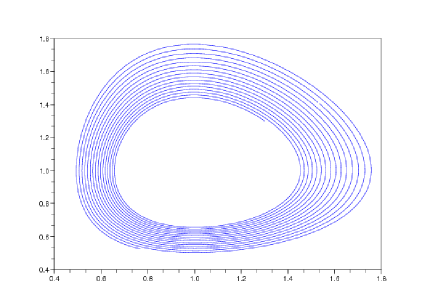
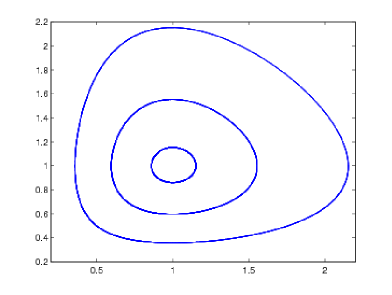
Figure 1: Left: a spiralling orbit of the explicit Euler method with the time-step $\epsilon=0.01$ applied to the Lotka-Volterra system. Right: three orbits of the Kahan’s discretization with $\epsilon=0.1$.

3 Hirota-Kimura bases and integrals

In this section a general formulation of a remarkable mechanism will be given, which seems to be responsible for the integrability of the Hirota-Kimura type (or Kahan type) discretizations of algebraically completely integrable systems. This mechanism is so far not well understood, in fact at the moment we do not know what mathematical structures make it actually work.

Throughout this section $f:{\mathbb{R}}^{n}\to{\mathbb{R}}^{n}$ is a birational map, while $h_{i},\varphi_{i}:{\mathbb{R}}^{n}\to{\mathbb{R}}$ stand for rational, usually polynomial functions on the phase space. We start with recalling a well known definition.

Definition 1

A function $h:{\mathbb{R}}^{n}\to{\mathbb{R}}$ is called an integral, or a conserved quantity, of the map $f$, if for every $x_{0}\in{\mathbb{R}}^{n}$ there holds

$$h(f(x))=h(x),$$

so that

$$h\circ f^{i}(x)=h(x)\quad\forall i\in{\mathbb{Z}}.$$

Convention. In the last formula and everywhere in the sequel, we use the expression $h\circ f^{i}(x)$ for the evaluation of the function $h\circ f^{i}$ at the point $x$. This is equivalent to $h(f^{i}(x))$ and is used to spare some parentheses.

Thus, each orbit of the map $f$ lies on a certain level set of its integral $h$. As a consequence, if one knows $d$ functionally independent integrals $h_{1},\ldots,h_{d}$ of $f$, one can claim that each orbit of $f$ is confined to an $(n-d)$-dimensional invariant set, which is a common level set of the functions $h_{1},\ldots,h_{d}$.

Definition 2

A set of functions $\Phi=(\varphi_{1},\ldots,\varphi_{l})$, linearly independent over ${\mathbb{R}}$, is called a Hirota-Kimura basis (HK-basis), if for every $x_{0}\in{\mathbb{R}}^{n}$ there exists a vector $c=(c_{1},\ldots,c_{l})\neq 0$ such that

$$(c_{1}\varphi_{1}+\ldots+c_{l}\varphi_{l})\circ f^{i}(x)=0\quad\forall i\in{\mathbb{Z}}.$$ (8)

For a given $x\in{\mathbb{R}}^{n}$, the set of all vectors $c\in{\mathbb{R}}^{l}$ with this property will be denoted by $K_{\Phi}(x)$ and called the null-space of the basis $\Phi$ (at the point $x$). This set clearly is a vector space.

Thus, for a HK-basis $\Phi$ and for $c\in K_{\Phi}(x)$ the function $h=c_{1}\varphi_{1}+...+c_{l}\varphi_{l}$ vanishes along the $f$-orbit of $x$. Let us stress that we cannot claim that $h=c_{1}\varphi_{1}+...+c_{l}\varphi_{l}$ is an integral of motion, since vectors $c\in K_{\Phi}(x)$ do not have to belong to $K_{\Phi}(y)$ for initial points $y$ not lying on the orbit of $x$. However, for any $x$ the orbit $\{f^{i}(x)\}$ is confined to the common zero level set of $d$ functions

$$h_{j}=c_{1}^{(j)}\varphi_{1}+\ldots+c_{l}^{(j)}\varphi_{l}=0,\quad j=1,\ldots,d,$$

where the vectors $c^{(j)}=\big{(}c_{1}^{(j)},\ldots,c_{l}^{(j)}\big{)}\in{\mathbb{R}}^{l}$ form a basis of $K_{\Phi}(x)$. Thus, knowledge of a HK-basis with the null-space of dimension $d$ leads to a similar conclusion as knowledge of $d$ independent integrals of $f$, namely to the conclusion that the orbits lie on $(n-d)$-dimensional invariant sets. Note, however, that a HK-basis gives no immediate information on how these invariant sets foliate the phase space ${\mathbb{R}}^{n}$, since the vectors $c^{(j)}$, and therefore the functions $h_{j}$, change from one initial point $x$ to another.

Although the notions of integrals and of HK-bases cannot be immediately translated into one another, they turn out to be closely related.

The simplest situation for a HK-basis corresponds to $l=2$, $\dim K_{\Phi}(x)=d=1$. In this case we immediately see that $h=\varphi_{1}/\varphi_{2}$ is an integral of motion of the map $f$. Conversely, for any rational integral of motion $h=\varphi_{1}/\varphi_{2}$ its numerator and denominator $\varphi_{1}$, $\varphi_{2}$ satisfy

$$(c_{1}\varphi_{1}+c_{2}\varphi_{2})\circ f^{i}(x)=0,\quad i\in{\mathbb{Z}},$$

with $c_{1}=1$, $c_{2}=-h(x)$, and thus build a HK-basis with $l=2$. Thus, the notion of a HK-basis generalizes (for $l\geq 3$) the notion of integrals of motion.

On the other hand, knowing a HK-basis $\Phi$ with $\dim K_{\Phi}(x)=d\geq 1$ allows one to find integrals of motion for the map $f$. Indeed, from Definition 2 there follows immediately:

Proposition 3

If $\Phi$ is a HK-basis for a map $f$, then

$$K_{\Phi}(f(x))=K_{\Phi}(x).$$

Thus, the $d$-dimensional null-space $K_{\Phi}(x)\in Gr(d,l)$, regarded as a function of the initial point $x\in{\mathbb{R}}^{n}$, is constant along trajectories of the map $f$, i.e., it is a $Gr(d,l)$-valued integral. One can extract from this fact a number of scalar integrals.

Corollary 4

Let $\Phi$ be a HK-basis for $f$ with $\dim K_{\Phi}(x)=d$ for all $x\in\mathbb{R}^{n}$. Take a basis of $K_{\Phi}(x)$ consisting of $d$ vectors $c^{(i)}\in{\mathbb{R}}^{l}$ and put them into the columns of a $l\times d$ matrix $C(x)$. For any $d$-index $\alpha=(\alpha_{1},\ldots,\alpha_{d})\subset\{1,2,\ldots,n\}$ let $C_{\alpha}=C_{\alpha_{1}\ldots\alpha_{d}}$ denote the $d\times d$ minor of the matrix $C$ built from the rows $\alpha_{1},\ldots,\alpha_{d}$. Then for any two $d$-indices $\alpha,\beta$ the function $C_{\alpha}/C_{\beta}$ is an integral of $f$.

Proof. The functions $C_{\alpha}$ are nothing other than the Grassmann-Plücker coordinates of the $d$-space $K_{\Phi}(x)$ in the Grassmannian $Gr(d,l)$, which are defined up to a common factor. More detailed, any basis of $K_{\Phi}(f(x))$ is obtained from the given basis of $K_{\Phi}(x)$ via a right multiplication of $C$ by a non-degenerate $d\times d$ matrix $D$. This yields a simultaneous multiplication of all $C_{\alpha}$ by the common factor $\det D$. This operation does not change the quotients $C_{\alpha}/C_{\beta}$. $\Box$

Especially simple is the situation when the null-space of a HK-basis has dimension $d=1$.

Corollary 5

Let $\Phi$ be a HK-basis for $f$ with $\dim K_{\Phi}(x)=1$ for all $x\in\mathbb{R}^{n}$. Let $K_{\Phi}(x)=[c_{1}(x):\ldots:c_{l}(x)]\in{\mathbb{R}}\mathbb{P}^{l-1}$. Then the functions $c_{j}/c_{k}$ are integrals of motion for $f$.

An interesting (and difficult) question is about the number of functionally independent integrals obtained from a given HK-basis according to Corollaries 4 and 5. We will see later that it is possible for a HK-basis with a one-dimensional null-space to produce more than one independent integral (see Theorem 13).

The first examples of this mechanism (with $d=1$) were found in [Kimura and Hirota 2000] and (somewhat implicitly) in [Hirota and Kimura 2000].

4 Finding Hirota-Kimura bases

At present, we cannot give any theoretical sufficient conditions for existence of a Hirota-Kimura basis $\Phi$ for a given map $f$, and the only way to find such a basis remains the experimental one. Definition 2 requires to verify condition (8) for all $i\in{\mathbb{Z}}$, which is, of course, impractical. We now show that it is enough to check this condition for a finite number of iterates $f^{i}$.

For a given set of functions $\Phi=(\varphi_{1},\ldots,\varphi_{l})$ and for any interval $[j,k]\subset{\mathbb{Z}}$ we denote

$$X_{[j,k]}(x)=\left(\begin{array}[]{ccc}\varphi_{1}(f^{j}(x))&..&\varphi_{l}(f^{j}(x))\\ \varphi_{1}(f^{j+1}(x))&..&\varphi_{l}(f^{j+1}(x))\\ ...&&...\\ \varphi_{1}(f^{k}(x))&..&\varphi_{l}(f^{k}(x))\end{array}\right).$$ (9)

In particular, $X_{(-\infty,\infty)}(x)$ will denote the double infinite matrix of the type (9). Obviously,

$$\ker X_{(-\infty,\infty)}(x)=K_{\Phi}(x).$$

Thus, Definition 2 requires that $\dim\ker X_{(-\infty,\infty)}(x)\geq 1$. Our algorithm for detecting this situation is based on the following observation.

Theorem 6

Let

$$\dim\ker X_{[0,s-1]}(x)=\left\{\begin{array}[]{cl}l-s&{\rm for}\;\;1\leq s\leq l-d,\\ d&{\rm for}\;\;s=l-d+1,\end{array}\right.$$ (10)

hold with some $d$ for all $x\in{\mathbb{R}}^{n}$. Then for any $x\in{\mathbb{R}}^{n}$ there holds:

$$\ker X_{(-\infty,\infty)}(x)=\ker X_{[0,l-d-1]}(x),$$

and, in particular,

$$\dim\ker X_{(-\infty,\infty)}(x)=d.$$

Proof. By definition, $X_{[j,k]}(x)=X_{[0,k-j]}(f^{j}(x))$. Therefore, applying condition (10) to iterates $f^{j}(x)$ instead of $x$ itself, we see that the kernel of any submatrix of $X_{(-\infty,\infty)}(x)$ with $l-d$ rows, as well as the kernel of any submatrix with $l-d+1$ rows, is $d$-dimensional:

$$\dim\ker X_{[j,j+l-d-1]}(x)=\dim\ker X_{[j,j+l-d]}(x)=\dim\ker X_{[j+1,j+l-d]}(x).$$

Since, obviously,

$$\ker X_{[j,j+l-d-1]}(x)\supset\ker X_{[j,j+l-d]}(x)\subset\ker X_{[j+1,j+l-d]}(x),$$

we find that all three kernels coincide, in particular,

$$\ker X_{[j,j+l-d-1]}(x)=\ker X_{[j+1,j+l-d]}(x).$$

By induction, all $\ker X_{[j,j+l-d-1]}(x)$, $j\in{\mathbb{Z}}$, coincide, and therefore they coincide with $\ker X_{(-\infty,\infty)}(x)$, as well. $\Box$

These results lead us to formulate the following numerical algorithm for the estimation of $\dim K_{\Phi}(x)$ for a hypothetic HK-basis $\Phi=(\varphi_{1},\ldots,\varphi_{l})$.

• For several randomly chosen initial points $x\in{\mathbb{R}}^{n}$, compute $\dim\ker X_{[0,s-1]}(x)$ for $1\leq s\leq l$. If for every $x$ condition (10) is satisfied with one and the same $d\geq 1$, then $\Phi$ is likely to be a HK-basis for $f$, with $\dim K_{\Phi}(x)=d$.

We stress once again that generally (for general maps $f$ and general monomial sets $\Phi$) one will find that the $l\times l$ matrix $X_{[0,l-1]}(x)$ is non-degenerate for a typical $x$, so that $\dim K_{\Phi}(x)=0$. Finding (a candidate for) a HK-basis $\Phi$ is a highly non-trivial task.

Having found a HK-basis $\Phi$ with $\dim K_{\Phi}(x)=d$ numerically, one faces the next problem: to prove this fact, that is, to prove that the system of equations (8) with $i=i_{0},i_{0}+1,\ldots,i_{0}+l-d$ admits (for some, and then for all $i_{0}\in{\mathbb{Z}}$) a $d$-dimensional space of solutions. For the sake of clarity, we restrict our following discussion to the most important case $d=1$. Thus, one has to prove that the homogeneous system

$$(c_{1}\varphi_{1}+\ldots+c_{l}\varphi_{l})\circ f^{i}(x)=0,\qquad i=i_{0},i_{0}+1,\ldots,i_{0}+l-1$$ (11)

admits for every $x\in{\mathbb{R}}^{n}$ a one-dimensional vector space of non-trivial solutions. The main obstruction for a symbolic solution of the system (11) is the growing complexity of the iterates $f^{i}(x)$. While the expression for $f(x)$ is typically of a moderate size, already the second iterate $f^{2}(x)$ becomes typically prohibitively big. In such a situation a symbolic solution of the linear system (11) should be considered as impossible, as soon as $f^{2}(x)$ is involved, for instance, if $l\geq 3$ and one considers the linear system with $i=0,1,\ldots,l-1$.

Therefore it becomes crucial to reduce the number of iterates involved in (11) as far as possible. A reduction of this number by 1 becomes in many cases crucial! One can imagine several ways to accomplish this.

• Take into account that, because of the reversibility $f^{-1}(x,\epsilon)=f(x,-\epsilon)$, the negative iterates $f^{-i}$ are of the same complexity as $f^{i}$. Therefore, one can reduce the complexity of the functions involved in (11) by choosing $i_{0}=-[l/2]$ instead of the naive choice $i_{0}=0$.

For instance, in the case $l=3$ one should consider the system (11) with $i=-1,0,1$, and not with $i=0,1,2$. However, already in the case $l=4$ this simple recipe does not allow us to avoid considering $f^{2}$. In this case, the following way of dealing with the system (11) becomes useful.

• Set $c_{l}=-1$ and consider instead of the homogeneous system (11) of $l$ equations the non-homogeneous system

  $$(c_{1}\varphi_{1}+\ldots+c_{l-1}\varphi_{l-1})\circ f^{i}(x)=\varphi_{l}\circ f^{i}(x),\quad i=i_{0},i_{0}+1,\ldots,i_{0}+l-2,\quad$$ (12)

  of $l-1$ equations. Having found the (unique) solution $\big{(}c_{1}(x),\ldots,c_{l-1}(x)\big{)}$, prove that these functions are integrals of motion, that is,

  $$c_{1}(f(x))=c_{1}(x),\quad\ldots,\quad c_{l-1}(f(x))=c_{l-1}(x).$$ (13)

Thus, for instance, in the case $l=4$ one has to deal with the non-homogeneous system of equations (12) with $i=-1,0,1$. Unfortunately, even if one is able to solve this system symbolically, the task of a symbolic verification of eq. (13) might become very hard due to complexity of the solutions $\big{(}c_{1}(x),\ldots,c_{l-1}(x)\big{)}$.

This is the way taken, for instance, in [Kimura and Hirota 2000]. In that paper, the task of verifying the equations of the type (13) for the discrete time Lagrange top is performed with the following method.

• In order to verify that a rational function $c(x)=p(x)/q(x)$ is an integral of motion of the map $\widetilde{x}=f(x)$ coming from a system (2):

  • find a Gröbner basis $G$ of the ideal $I$ generated by the components of eq. (2), considered as multi-linear polynomials of $2n$ variables $x,\widetilde{x}$ of total degree 2;

  • check, via polynomial division through elements of $G$, whether the polynomial $\delta(x,\widetilde{x})=p(\widetilde{x})q(x)-p(x)q(\widetilde{x})$ belongs to the ideal $I$.

An advantage of this method is that neither of its two steps needs the complicated explicit expressions for the map $f$. Nevertheless, both steps might be very demanding, especially the second step in case of a complicated integral $c(x)$.

Sometimes, the task of verifying equations (13) can be circumvented by means of the following tricks.

• Solve system (12) for two different but overlapping ranges $i\in[i_{0},i_{0}+l-2]$ and $i\in[i_{1},i_{1}+l-2]$. If the solutions coincide, then eq. (13) holds automatically.

Indeed, in this situation the functions $\big{(}c_{1}(x),\ldots,c_{l-1}(x)\big{)}$ solve the system with $i\in[i_{0},i_{0}+l-2]\cup[i_{1},i_{1}+l-2]$ consisting of more than $l-1$ equations.

A clever modification of this idea, which allows one to avoid solving the second system, is as follows.

• Suppose that the index range $i\in[i_{0},i_{0}+l-2]$ in eq. (12) contains 0 but is non-symmetric. If the solution of this system $\big{(}c_{1}(x,\epsilon),\ldots,c_{l-1}(x,\epsilon)\big{)}$ is even with respect to $\epsilon$, then eqs. (13) hold automatically.

Indeed, the reversibility of the map $f^{-1}(x,\epsilon)=f(x,-\epsilon)$ yields in this case that equations of the system (12) are satisfied for $i\in[-(i_{0}+l-2),-i_{0}]$, as well, and the intervals $[i_{0},i_{0}+l-2]$ and $[-(i_{0}+l-2),-i_{0}]$ overlap but do not coincide, by condition.

Finally, the most powerful method of reducing the number of iterations to be considered is as follows.

• Often, the solutions $\big{(}c_{1}(x),\ldots,c_{l-1}(x)\big{)}$ satisfy some linear relations with constant coefficients. Find (observe) such relations numerically. Each such (still hypothetic) relation can be used to replace one equation in the system (12). Solve the resulting system symbolically, and proceed as in recipes (C) or (D) in order to verify eqs. (13).

In some (rare) cases the integrals found by this approach are nice and simple enough to enable one to verify eqs. (13) directly. Of course, it would be highly desirable to find some structures, like Lax representation, bi-Hamiltonian structure, etc., which would allow one to check the conservation of integrals in a more clever way, but up to now no such structures have been found for any of the Hirota-Kimura-type discretizations.

5 Hirota-Kimura discretization of the Euler top

We now illustrate the Hirota-Kimura mechanism by its application to the Euler top. This three-dimensional system is simple enough to enable one to perform all necessary computations symbolically, even by hand. At the same time, it provides a perfect illustration for many of the issues mentioned in the previous section.

5.1 Euler top

The differential equations of motion of the Euler top read

$$\dot{x}_{1}=\alpha_{1}x_{2}x_{3},\quad\dot{x}_{2}=\alpha_{2}x_{3}x_{1},\quad\dot{x}_{3}=\alpha_{3}x_{1}x_{2},$$ (14)

with $\alpha_{i}$ being real parameters of the system. This is one of the most famous integrable systems of the classical mechanics, with a big literature devoted to it. We mention only that this system can be explicitly integrated in terms of elliptic functions, and admits two functionally independent integrals of motion. Actually, a quadratic function $H(x)=\gamma_{1}x_{1}^{2}+\gamma_{2}x_{2}^{2}+\gamma_{3}x_{3}^{2}$ is an integral for eqs. (14), if $\langle\gamma,\alpha\rangle=\gamma_{1}\alpha_{1}+\gamma_{2}\alpha_{2}+\gamma_{2}\alpha_{2}=0$. In particular, the following three functions are integrals of motion:

$$H_{1}=\alpha_{3}x_{2}^{2}-\alpha_{2}x_{3}^{2},\qquad H_{2}=\alpha_{1}x_{3}^{2}-\alpha_{3}x_{1}^{2},\qquad H_{3}=\alpha_{2}x_{1}^{2}-\alpha_{1}x_{2}^{2}.$$

Clearly, only two of them are functionally independent because of $\alpha_{1}H_{1}+\alpha_{2}H_{2}+\alpha_{3}H_{3}=0$.

5.2 Discrete equations of motion

The Hirota-Kimura discretization of the Euler top introduced in [Hirota and Kimura 2000] reads as

$$\left\{\begin{array}[]{l}\widetilde{x}_{1}-x_{1}=\epsilon\alpha_{1}(\widetilde{x}_{2}x_{3}+x_{2}\widetilde{x}_{3}),\\ \widetilde{x}_{2}-x_{2}=\epsilon\alpha_{2}(\widetilde{x}_{3}x_{1}+x_{3}\widetilde{x}_{1}),\\ \widetilde{x}_{3}-x_{3}=\epsilon\alpha_{3}(\widetilde{x}_{1}x_{2}+x_{1}\widetilde{x}_{2}).\end{array}\right.$$ (15)

Thus, the map $f:x\mapsto\widetilde{x}$ obtained by solving (15) for $\widetilde{x}$, is given by:

$$\widetilde{x}=f(x,\epsilon)=A^{-1}(x,\epsilon)x,\qquad A(x,\epsilon)=\begin{pmatrix}1&-\epsilon\alpha_{1}x_{3}&-\epsilon\alpha_{1}x_{2}\\ -\epsilon\alpha_{2}x_{3}&1&-\epsilon\alpha_{2}x_{1}\\ -\epsilon\alpha_{3}x_{2}&-\epsilon\alpha_{3}x_{1}&1\end{pmatrix}.$$ (16)

It might be instructive to have a look at the explicit formulas for this map:

$$\left\{\begin{array}[]{l}\widetilde{x}_{1}=\dfrac{x_{1}+2\epsilon\alpha_{1}x_{2}x_{3}+\epsilon^{2}x_{1}(-\alpha_{2}\alpha_{3}x_{1}^{2}+\alpha_{3}\alpha_{1}x_{2}^{2}+\alpha_{1}\alpha_{2}x_{3}^{2})}{\Delta(x,\epsilon)}\,,\\ \\ \widetilde{x}_{2}=\dfrac{x_{2}+2\epsilon\alpha_{2}x_{3}x_{1}+\epsilon^{2}x_{2}(\alpha_{2}\alpha_{3}x_{1}^{2}-\alpha_{3}\alpha_{1}x_{2}^{2}+\alpha_{1}\alpha_{2}x_{3}^{2})}{\Delta(x,\epsilon)}\,,\\ \\ \widetilde{x}_{3}=\dfrac{x_{3}+2\epsilon\alpha_{3}x_{1}x_{2}+\epsilon^{2}x_{3}(\alpha_{2}\alpha_{3}x_{1}^{2}+\alpha_{3}\alpha_{1}x_{2}^{2}-\alpha_{1}\alpha_{2}x_{3}^{2})}{\Delta(x,\epsilon)}\,,\end{array}\right.$$ (17)

where

$$\Delta(x,\epsilon)=\det A(x,\epsilon)=1-\epsilon^{2}(\alpha_{2}\alpha_{3}x_{1}^{2}+\alpha_{3}\alpha_{1}x_{2}^{2}+\alpha_{1}\alpha_{2}x_{3}^{2})-2\epsilon^{3}\alpha_{1}\alpha_{2}\alpha_{3}x_{1}x_{2}x_{3}.$$

As always the case for HK-type discretizations, this map is birational, and there holds the reversibility property:

$$f^{-1}(x,\epsilon)=f(x,-\epsilon).$$

Apart from the Lax representation which is still missing, the discretization (16) exhibits all the usual features of an integrable map: an invariant volume form, a bi-Hamiltonian structure (that is, two compatible invariant Poisson structures), two functionally independent conserved quantities in involution, and solutions in terms of elliptic functions. The difference of its qualitative behavior as compared with non-integrable discretizations is striking, cf. Fig. 2. For further details about the properties of this discretization we refer to [Hirota and Kimura 2000] and [Petrera and Suris 2008].

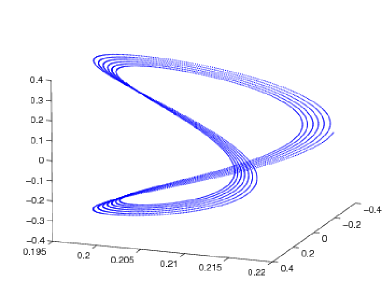
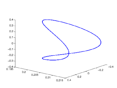
Figure 2: Left: a spiralling orbit of the explicit Euler method with the time-step $\epsilon=0.3$ applied to the Euler top. Right: a single orbit of the Hirota-Kimura discretization with the same time-step, lying on an invariant spatial elliptic curve (intersection of two quadrics).

The integrals have been first found in [Hirota and Kimura 2000], apparently with the help of the approach discussed in the present work. However, since the resulting integrals are sufficiently simple and nice, their conservation can be easily verified by hands, therefore the paper [Hirota and Kimura 2000] presents them in an ad hoc form, without explaining how they have been discovered. We now try to reconstruct the way the results of [Hirota and Kimura 2000] were originally found. For this aim, we apply to the map (16) the method described in section 3.

5.3 Hirota-Kimura bases

Since all integrals of the Euler top are linear combinations of the functions $x_{k}^{2}$, it is natural to try the set

$$\Phi=(x_{1}^{2},x_{2}^{2},x_{3}^{2},1)$$ (18)

as a HK-basis for the discrete time Euler top. An application of the numerical algorithm (N) suggests that the following statement holds:

Theorem 7

The set (18) is a HK-basis for the map (16) with $\dim K_{\Phi}(x)=2$. Therefore, any orbit of this map lies on the intersection of two quadrics in ${\mathbb{R}}^{3}$.

We will prove this theorem by finding two smaller HK-bases with $d=1$. Namely, application of the numerical algorithm (N) suggests that omitting any one of the four functions $1$, $x_{k}^{2}$ from the basis $\Phi$ leads to a HK-basis with $d=1$. In other words, for every $x\in{\mathbb{R}}^{3}$ there exists a one-dimensional space of vectors $(c_{1},c_{2},c_{3})$ such that

$$(c_{1}x_{1}^{2}+c_{2}x_{2}^{2}+c_{3}x_{3}^{2})\circ f^{i}(x)=0,\qquad i\in{\mathbb{Z}},$$

as well as a one-dimensional space of vectors $(d_{1},d_{2},d_{4})$ such that

$$(d_{1}x_{1}^{2}+d_{2}x_{2}^{2}+d_{4})\circ f^{i}(x)=0,\qquad i\in{\mathbb{Z}}.$$

These numerical results can be now proven analytically.

Proposition 8

The set

$$\Phi_{0}=(x_{1}^{2},x_{2}^{2},x_{3}^{2})$$

is a HK-basis for the map (16) with $\dim K_{\Phi_{0}}(x)=1$. At each point $x\in{\mathbb{R}}^{3}$ there holds:

$$K_{\Phi_{0}}(x)=[c_{1}:c_{2}:c_{3}]=[\,\alpha_{3}x_{2}^{2}-\alpha_{2}x_{3}^{2}:\alpha_{1}x_{3}^{2}-\alpha_{3}x_{1}^{2}:\alpha_{2}x_{1}^{2}-\alpha_{1}x_{2}^{2}\,].$$

Setting $c_{3}=-1$, the functions

$$c_{1}(x)=\frac{\alpha_{3}x_{2}^{2}-\alpha_{2}x_{3}^{2}}{\alpha_{1}x_{2}^{2}-\alpha_{2}x_{1}^{2}},\qquad c_{2}(x)=\frac{\alpha_{1}x_{3}^{2}-\alpha_{3}x_{1}^{2}}{\alpha_{1}x_{2}^{2}-\alpha_{2}x_{1}^{2}}$$ (19)

are integrals of motion of the map (16).

Proof. We proceed according to the recipe (B), set $c_{3}=-1$, and solve symbolically the system

$$(c_{1}x_{1}^{2}+c_{2}x_{2}^{2})\circ f^{i}(x)=x_{3}^{2}\circ f^{i}(x),\quad i=0,1,$$ (20)

which involves two non-homogeneous equations for two unknowns. System (20) can be written as

$$\left\{\begin{array}[]{ccl}c_{1}x_{1}^{2}+c_{2}x_{2}^{2}&=&x_{3}^{2},\\ c_{1}\widetilde{x}_{1}^{2}+c_{2}\widetilde{x}_{2}^{2}&=&\widetilde{x}_{3}^{2},\end{array}\right.$$ (21)

where, of course, explicit formulas (17) have to be used for $\widetilde{x}_{k}$. The solution of this system is given by formulas (19). The components of the solution do not depend on $\epsilon$, therefore, according to the recipe (D), we conclude that functions (19) are integrals of motion of the map (16). $\Box$

It should be mentioned that the independence of the solution $(c_{1},c_{2})$ on $\epsilon$, or, more generally, the dependence through even powers of $\epsilon$ only, which will be mentioned on many occasions below, starting with Proposition 9, is not granted by any well-understood mechanism. Rather, it is just an instance of very remarkable and miraculous cancellations of non-even polynomials. We illustrate this phenomenon by providing additional details to the previous proof. The solution of eqs. (21) by the Cramer’s rule is given by ratios of determinants of the type

$$\left|\begin{array}[]{cc}x_{i}^{2}&x_{j}^{2}\\ \widetilde{x}_{i}^{2}&\widetilde{x}_{j}^{2}\end{array}\right|=\frac{4\epsilon(\alpha_{j}x_{i}^{2}-\alpha_{i}x_{j}^{2})(x_{1}+\epsilon\alpha_{1}x_{2}x_{3})(x_{2}+\epsilon\alpha_{2}x_{3}x_{1})(x_{3}+\epsilon\alpha_{3}x_{1}x_{2})}{\Delta^{2}(x,\epsilon)}$$ (22)

In the ratios of such determinants everything cancels out, except for the factors $\alpha_{j}x_{i}^{2}-\alpha_{i}x_{j}^{2}$. The cancellation of the denominators $\Delta^{2}(x,\epsilon)$ is, of course, no wonder, but the cancellation of the non-even factors in the numerators is rather miraculous.

One more typical phenomenon occurs in Proposition 8: although we have found apparently two integrals of motion (19), they turn out to be functionally dependent. Indeed, there holds an identity

$$\alpha_{1}c_{1}(x)+\alpha_{2}c_{2}(x)=\alpha_{3},$$

so that for each $x\in{\mathbb{R}}^{3}$ the space $K_{\Phi_{0}}(x)$ is orthogonal to the constant vector $(\alpha_{1},\alpha_{2},\alpha_{3})$. If one would have guessed this relation numerically, one could simplify the computation of the integrals $c_{1},c_{2}$ by considering the system

$$\left\{\begin{array}[]{ccl}c_{1}x_{1}^{2}+c_{2}x_{2}^{2}&=&x_{3}^{2},\\ c_{1}\alpha_{1}+c_{2}\alpha_{2}&=&\alpha_{3},\end{array}\right.$$ (23)

instead of (21). Observe that existence of a linear relation allows one to reduce a number of iterates of $f$ involved in the linear system (in the present situation, the system (23) contains no iterates of $f$ at all!). The latter system would lead to the same formulas (19), however, in this case one could not argue as in (D), and would be forced to prove that the functions (19) are integrals of motion directly, by verifying for them equations (13).

Anyway, the existence of the HK-basis $\Phi_{0}$ yields existence of only one independent integral of the map $f$, which is not enough to assure the integrability of $f$.

Proposition 9

The set

$$\Phi_{1}=(x_{1}^{2},x_{2}^{2},1)$$

is a HK-basis for the map (16) with $\dim K_{\Phi_{1}}(x)=1$. At each point $x\in{\mathbb{R}}^{3}$ there holds:

$$K_{\Phi_{1}}(x)=[d_{1}:d_{2}:-1],$$

where

$$d_{1}(x)=\frac{\alpha_{2}(1-\epsilon^{2}\alpha_{3}\alpha_{1}x_{2}^{2})}{\alpha_{2}x_{1}^{2}-\alpha_{1}x_{2}^{2}}\,,\qquad d_{2}(x)=\frac{\alpha_{1}(1-\epsilon^{2}\alpha_{2}\alpha_{3}x_{1}^{2})}{\alpha_{1}x_{2}^{2}-\alpha_{2}x_{1}^{2}}\,.$$ (24)

These functions are integrals of motion of the map (16).

Proof. Following again prescription (B), we set $d_{4}=-1$, and solve symbolically the non-homogeneous system

$$(d_{1}x_{1}^{2}+d_{2}x_{2}^{2})\circ f^{i}(x)=1,\quad i=0,1,$$

or

$$\left\{\begin{array}[]{ccl}d_{1}x_{1}^{2}+d_{2}x_{2}^{2}&=&1,\\ d_{1}\widetilde{x}_{1}^{2}+d_{2}\widetilde{x}_{2}^{2}&=&1.\end{array}\right.$$

The solution is given by eq. (24), due to eq. (22) and

$$\left|\begin{array}[]{cc}1&x_{i}^{2}\\ 1&\widetilde{x}_{i}^{2}\end{array}\right|=\frac{4\epsilon\alpha_{i}(1-\epsilon^{2}\alpha_{j}\alpha_{k}x_{i}^{2})(x_{1}+\epsilon\alpha_{1}x_{2}x_{3})(x_{2}+\epsilon\alpha_{2}x_{3}x_{1})(x_{3}+\epsilon\alpha_{3}x_{1}x_{2})}{\Delta^{2}(x,\epsilon)}$$

This time its components do depend on $\epsilon$, but are manifestly even functions of $\epsilon$. Everything non-even luckily cancels, again. Therefore, the argument (D) is still applicable, so that the functions (24) are integrals of motion of the map $f$. $\Box$

Functions (24) are again functionally dependent, because of

$$\alpha_{1}d_{1}(x)+\alpha_{2}d_{2}(x)=\epsilon^{2}\alpha_{1}\alpha_{2}\alpha_{3}.$$

However, they are, clearly, functionally independent on the previously found functions (19), because $c_{1},c_{2}$ depend on $x_{3}$, while $d_{1},d_{2}$ do not.

Of course, the permutational symmetry yields that each of the sets of monomials $\Phi_{2}=(x_{2}^{2},x_{3}^{2},1)$ and $\Phi_{3}=(x_{1}^{2},x_{3}^{2},1)$ is a HK-basis, as well, with $\dim K_{\Phi_{2}}(x)=\dim K_{\Phi_{3}}(x)=1$. Any two of the four found one-dimensional null-spaces span the full null-space $K_{\Phi}(x)$. In particular, $K_{\Phi_{0}}(x)$ lies in $K_{\Phi_{1}}(x)\oplus K_{\Phi_{2}}(x)$.

Summarizing, we have found a HK-basis with a two-dimensional null-space, as well as two functionally independent conserved quantities for the HK-discretization of the Euler top. Both results yield integrability of this discretization, in the sense that its orbits are confined to closed curves in ${\mathbb{R}}^{3}$. Moreover, each such curve is an intersection of two quadrics, which in the general position case is an elliptic curve.

6 Hirota-Kimura-type discretization of the Clebsch system

6.1 Clebsch system

The motion of a rigid body in an ideal fluid can be described by the so called Kirchhoff equations [Kirchhoff 1870]:

$$\left\{\begin{array}[]{l}\dot{m}=m\times\dfrac{\partial H}{\partial m}+p\times\dfrac{\partial H}{\partial p},\\ \dot{p}=p\times\dfrac{\partial H}{\partial m},\end{array}\right.$$ (25)

with $H$ being a quadratic form in $m=(m_{1},m_{2},m_{3})\in{\mathbb{R}}^{3}$ and $p=(p_{1},p_{2},p_{3})\in{\mathbb{R}}^{3}$; here $\times$ denotes vector product in ${\mathbb{R}}^{3}$. The physical meaning of $m$ is the total angular momentum, whereas $p$ represents the total linear momentum of the system. System (25) is Hamiltonian with the Hamilton function $H(m,p)$, with respect to the Poisson bracket

$$\{m_{i},m_{j}\}=m_{k},\qquad\{m_{i},p_{j}\}=p_{k},$$ (26)

where $(i,j,k)$ is a cyclic permutation of (1,2,3) (all other pairwise Poisson brackets of the coordinate functions are obtained from these by the skew-symmetry, or otherwise vanish). A detailed introduction to the general context of rigid body dynamics and its mathematical foundations can be found in [Marsden and Ratiu 1999].

A famous integrable case of the Kirchhoff equations was discovered in [Clebsch 1870] and is characterized by the Hamilton function $H=\frac{1}{2}\sum_{i=1}^{3}(m_{i}^{2}+\omega_{i}p_{i}^{2})$. The corresponding equations of motion read:

$$\left\{\begin{array}[]{l}\dot{m}=p\times\Omega p,\\ \dot{p}=p\times m,\end{array}\right.$$

where $\Omega={\rm diag}(\omega_{1},\omega_{2},\omega_{3})$ is the matrix of parameters, or in components:

$$\dot{m}_{1} = (\omega_{3}-\omega_{2})p_{2}p_{3},$$

$$\dot{m}_{2} = (\omega_{1}-\omega_{3})p_{3}p_{1},$$

$$\dot{m}_{3} = (\omega_{2}-\omega_{1})p_{1}p_{2},$$

$$\dot{p}_{1} = m_{3}p_{2}-m_{2}p_{3},$$

$$\dot{p}_{2} = m_{1}p_{3}-m_{3}p_{1},$$

$$\dot{p}_{3} = m_{2}p_{1}-m_{1}p_{2}.$$

This is the system which will be called the Clebsch system hereafter. For an embedding of this system into the modern theory of integrable systems see [Perelomov 1990, Reyman and Semenov-Tian-Shansky 1994]. The Clebsch system possesses four independent quadratic integrals:

$$H_{1} = m_{1}^{2}+m_{2}^{2}+m_{3}^{2}+\omega_{1}p_{1}^{2}+\omega_{2}p_{2}^{2}+\omega_{3}p_{3}^{2},$$ (27)

$$H_{2} = \omega_{1}m_{1}^{2}+\omega_{2}m_{2}^{2}+\omega_{3}m_{3}^{2}-\omega_{2}\omega_{3}p_{1}^{2}-\omega_{3}\omega_{1}p_{2}^{2}-\omega_{1}\omega_{2}p_{3}^{2},$$ (28)

$$H_{3} = p_{1}^{2}+p_{2}^{2}+p_{3}^{2},$$ (29)

$$H_{4} = m_{1}p_{1}+m_{2}p_{2}+m_{3}p_{3}.$$ (30)

These integrals are in involution with respect to the bracket (26), moreover, $H_{3},H_{4}$ are its Casimir functions (are in involution with any function on the phase space). However, the Hamiltonian structure will not play any role in the present paper. The set of linear combinations of the quadratic Hamiltonians $H_{1},H_{2},H_{3}$ coincides with the set of linear combinations of the functions

$$I_{1} = p_{1}^{2}+\frac{m_{2}^{2}}{\omega_{1}-\omega_{3}}+\frac{m_{3}^{2}}{\omega_{1}-\omega_{2}}\,,$$

$$I_{2} = p_{2}^{2}+\frac{m_{1}^{2}}{\omega_{2}-\omega_{3}}+\frac{m_{3}^{2}}{\omega_{2}-\omega_{1}}\,,$$

$$I_{3} = p_{3}^{2}+\frac{m_{1}^{2}}{\omega_{3}-\omega_{2}}+\frac{m_{2}^{2}}{\omega_{3}-\omega_{1}}\,.$$

For instance,

$$H_{1}=\omega_{1}I_{1}+\omega_{2}I_{2}+\omega_{3}I_{3},\quad H_{1}=-\omega_{2}\omega_{3}I_{1}-\omega_{3}\omega_{1}I_{2}-\omega_{1}\omega_{2}I_{3},\quad H_{3}=I_{1}+I_{2}+I_{3}.$$

6.2 Discrete equations of motion

Applying the Hirota-Kimura (or Kahan) approach to the Clebsch system, we arrive at the following discretization, proposed in [Ratiu 2006]:

$$\widetilde{m}_{1}-m_{1} = \epsilon(\omega_{3}-\omega_{2})(\widetilde{p}_{2}p_{3}+p_{2}\widetilde{p}_{3}),$$

$$\widetilde{m}_{2}-m_{2} = \epsilon(\omega_{1}-\omega_{3})(\widetilde{p}_{3}p_{1}+p_{3}\widetilde{p}_{1}),$$

$$\widetilde{m}_{3}-m_{3} = \epsilon(\omega_{2}-\omega_{1})(\widetilde{p}_{1}p_{2}+p_{1}\widetilde{p}_{2}),$$

$$\widetilde{p}_{1}-p_{1} = \epsilon(\widetilde{m}_{3}p_{2}+m_{3}\widetilde{p}_{2})-\epsilon(\widetilde{m}_{2}p_{3}+m_{2}\widetilde{p}_{3}),$$

$$\widetilde{p}_{2}-p_{2} = \epsilon(\widetilde{m}_{1}p_{3}+m_{1}\widetilde{p}_{3})-\epsilon(\widetilde{m}_{3}p_{1}+m_{3}\widetilde{p}_{1}),$$

$$\widetilde{p}_{3}-p_{3} = \epsilon(\widetilde{m}_{2}p_{1}+m_{2}\widetilde{p}_{1})-\epsilon(\widetilde{m}_{1}p_{2}+m_{1}\widetilde{p}_{2}).$$

In matrix form this can be put as

$$M(m,p,\epsilon)\begin{pmatrix}\widetilde{m}\\ \widetilde{p}\end{pmatrix}=\begin{pmatrix}m\\ p\end{pmatrix},$$

where

$$M(m,p,\epsilon)=\begin{pmatrix}1&0&0&0&\epsilon\omega_{23}p_{3}&\epsilon\omega_{23}p_{2}\\ 0&1&0&\epsilon\omega_{31}p_{3}&0&\epsilon\omega_{31}p_{1}\\ 0&0&1&\epsilon\omega_{12}p_{2}&\epsilon\omega_{12}p_{1}&0\\ 0&\epsilon p_{3}&-\epsilon p_{2}&1&-\epsilon m_{3}&\epsilon m_{2}\\ -\epsilon p_{3}&0&\epsilon p_{1}&\epsilon m_{3}&1&-\epsilon m_{1}\\ \epsilon p_{2}&-\epsilon p_{1}&0&-\epsilon m_{2}&\epsilon m_{1}&1\end{pmatrix},$$

and the abbreviation $\omega_{ij}=\omega_{i}-\omega_{j}$ is used. The solution of this $6\times 6$ linear system yields the birational map $f:{\mathbb{R}}^{6}\to{\mathbb{R}}^{6}$,

$$\begin{pmatrix}\widetilde{m}\\ \widetilde{p}\end{pmatrix}=f(m,p,\epsilon)=M^{-1}(m,p,\epsilon)\begin{pmatrix}m\\ p\end{pmatrix},$$ (31)

called hereafter the discrete Clebsch system. As usual, the reversibility property holds:

$$f^{-1}(m,p,\epsilon)=f(m,p,-\epsilon).$$ (32)

A remark on the complexity of the iterates of $f$ is in order here. Each component of $(\widetilde{m},\widetilde{p})=f(m,p)$ is a rational function with the numerator and the denominator being polynomials on $m_{k},p_{k}$ of total degree 6. The numerators of $\widetilde{p}_{k}$ consist of 31 monomials, the numerators of $\widetilde{m}_{k}$ consist of 41 monomials, the common denominator consists of 28 monomials. It should be taken into account that the coefficients of all these polynomials depend, in turn, polynomially on $\epsilon$ and $\omega_{k}$, which additionally increases their complexity for a symbolic manipulator. Expressions for the second iterate swell to astronomical length prohibiting naive attempts to compute them symbolically. Using MAPLE’s LargeExpressions package [Carette et al. 2006] and an appropriate veiling strategy it is however possible to obtain $f^{2}(m,p)$ with a reasonable amount of memory. Some impression on the complexity can be obtained from Table 1. The resulting expressions are too big to be used in further symbolic computations. Consider, for instance, the numerator of the $p_{1}$-component of $f^{2}(m,p)$. As a polynomial of $m_{k},p_{k}$, it contains 64 056 monomials; their coefficients are, in turn, polynomials of $\epsilon$ and $\omega_{k}$, and, considered as a polynomial of the phase variables and the parameters, this expression contains 1 647 595 terms.

	deg	$\deg_{p_{1}}$	$\deg_{p_{2}}$	$\deg_{p_{3}}$	$\deg_{m_{1}}$	$\deg_{m_{2}}$	$\deg_{m_{3}}$
Common denominator of $f^{2}$	27	24	24	24	12	12	12
Numerator of $p_{1}$-comp. of $f^{2}$	27	25	24	24	12	12	12
Numerator of $p_{2}$-comp. of $f^{2}$	27	24	25	24	12	12	12
Numerator of $p_{3}$-comp. of $f^{2}$	27	24	24	25	12	12	12
Numerator of $m_{1}$-comp. of $f^{2}$	33	28	28	28	15	14	14
Numerator of $m_{2}$-comp. of $f^{2}$	33	28	28	28	14	15	14
Numerator of $m_{3}$-comp. of $f^{2}$	33	28	28	28	14	14	15

Table 1: Degrees of the numerators and the denominator of the second iterate $f^{2}(m,p)$

6.3 Phase portrait and integrability

We now address the problem whether the discrete Clebsch system is integrable. Figs. 3 and 4 show plots of the discrete Clebsch system (31), produced with MATLAB, for two different sets of parameters values. These plots indicate a quite regular behavior of the orbits of the discrete Clebsch system. Each orbit seems to fill out a two-dimensional surface in the 6-dimensional phase space. Leaving aside the Hamiltonian aspects of integrability, we are interested just in this simpler issue: do orbits of the map (31) lie on two-dimensional surfaces in ${\mathbb{R}}^{6}$? A usual way to establish such a property would be to establish the existence of four functionally independent conserved quantities for this map. (We note in passing that plots of orbits are not very reliable in deciding about integrability. For instance, there are indications that the Kahan’s discretization (6) of the Lotka-Volterra system is non-integrable, even if its orbits visually lie on closed curves in the phase plane. A strong magnification unveils the existence of very small regions in the phase plane with a chaotic behavior.)

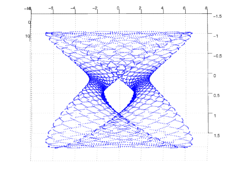
(a) $m_{1},m_{2},m_{3}$

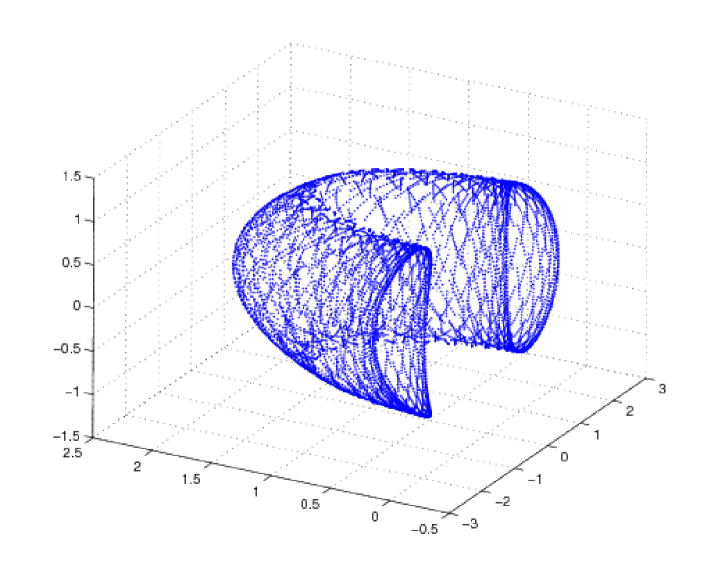
(b) $p_{1},p_{2},p_{3}$

Figure 3: An orbit of the discrete Clebsch system with $\omega_{1}=1$, $\omega_{2}=0.2$, $\omega_{3}=30$ and $\epsilon=1$; initial point $(m_{0},p_{0})=(1,1,1,1,1,1)$.

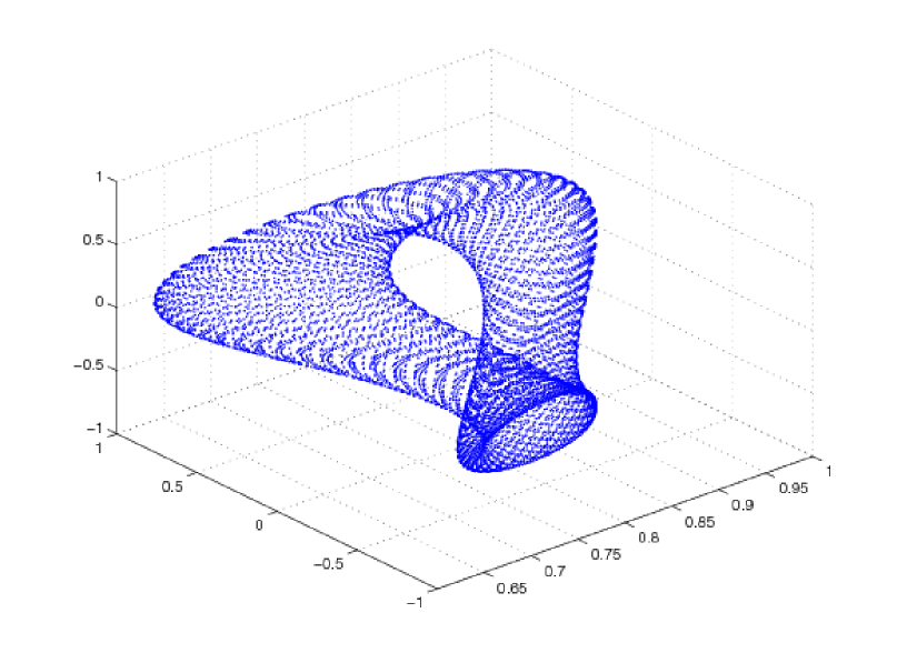
(a) $m_{1},m_{2},m_{3}$

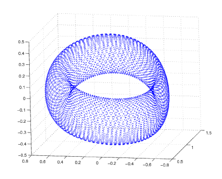
(b) $p_{1},p_{2},p_{3}$

Figure 4: An orbit of the discrete Clebsch system with $\omega_{1}=0.1$, $\omega_{2}=0.2$, $\omega_{3}=0.3$ and $\epsilon=1$; initial point $(m_{0},p_{0})=(1,1,1,1,1,1)$.

We will show that the answer to the above question is in affirmative. For this aim, we apply the approach based on the notion of HK-basis. As a first step, we apply the numerical algorithm (N) to the maximal set of monomials, which includes all monomials of which the integrals (27)–(30) of the continuous Clebsch system are built:

$$\varphi_{1}(m,p)=p_{1}^{2},\quad\varphi_{2}(m,p)=p_{2}^{2},\quad\varphi_{3}(m,p)=p_{3}^{2},$$

$$\varphi_{4}(m,p)=m_{1}^{2},\quad\varphi_{5}(m,p)=m_{2}^{2},\quad\varphi_{6}(m,p)=m_{3}^{2},$$

$$\varphi_{7}(m,p)=m_{1}p_{1},\quad\varphi_{8}(m,p)=m_{2}p_{2},\quad\varphi_{9}(m,p)=m_{3}p_{3},$$

$$\varphi_{10}(m,p)=1.$$

We come to the following result:

Theorem 10

The set of functions

$$\Phi=(p_{1}^{2},p_{2}^{2},p_{3}^{2},m_{1}^{2},m_{2}^{2},m_{3}^{2},m_{1}p_{1},m_{2}p_{2},m_{3}p_{3},1)$$

is a HK-basis for the map (31), with $\dim K_{\Phi}(m,p)=4$. Thus, any orbit of the map (31) lies on an intersection of four quadrics in ${\mathbb{R}}^{6}$.

At this point Theorem 10 remains a numerical result, based on the algorithm (N). A direct symbolical proof of this statement is impossible, since it requires dealing with $f^{i}$, $i\in[-4,4]$, and the fourth iterate $f^{4}$ is a forbiddingly large expression. In order to prove Theorem 10 and to extract from it four independent integrals of motion, it is desirable to find HK-(sub)bases with a smaller number of monomials, corresponding to some (preferably one-dimensional) subspaces of $K_{\Phi}(m,p)$. A much more detailed information on the HK-bases is provided by the following statement.

Theorem 11

The following four sets of functions are HK-bases for the map (31) with one-dimensional null-spaces:

$$\Phi_{0} = (p_{1}^{2},p_{2}^{2},p_{3}^{2},1),$$ (33)

$$\Phi_{1} = (p_{1}^{2},p_{2}^{2},p_{3}^{2},m_{1}^{2},m_{2}^{2},m_{3}^{2},m_{1}p_{1}),$$ (34)

$$\Phi_{2} = (p_{1}^{2},p_{2}^{2},p_{3}^{2},m_{1}^{2},m_{2}^{2},m_{3}^{2},m_{2}p_{2}),$$ (35)

$$\Phi_{3} = (p_{1}^{2},p_{2}^{2},p_{3}^{2},m_{1}^{2},m_{2}^{2},m_{3}^{2},m_{3}p_{3}).$$ (36)

If all the null-spaces are considered as subspaces of $\,{\mathbb{R}}^{10}$, so that

$$\begin{array}[]{cclrrrrrrrrr}K_{\Phi_{0}}&=&[c_{1}:&c_{2}:&c_{3}:&0:&0:&0:&0:&0:&0:&c_{10}],\\ K_{\Phi_{1}}&=&[\alpha_{1}:&\alpha_{2}:&\alpha_{3}:&\alpha_{4}:&\alpha_{5}:&\alpha_{6}:&\alpha_{7}:&0:&0:&0],\\ K_{\Phi_{2}}&=&[\beta_{1}:&\beta_{2}:&\beta_{3}:&\beta_{4}:&\beta_{5}:&\beta_{6}:&0:&\beta_{8}:&0:&0],\\ K_{\Phi_{3}}&=&[\gamma_{1}:&\gamma_{2}:&\gamma_{3}:&\gamma_{4}:&\gamma_{5}:&\gamma_{6}:&0:&0:&\gamma_{9}:&0],\end{array}$$

then there holds:

$$K_{\Phi}=K_{\Phi_{0}}\oplus K_{\Phi_{1}}\oplus K_{\Phi_{2}}\oplus K_{\Phi_{3}}.$$

Also this statement was first found with the help of numerical experiments based on the algorithm (N). In what follows, we will discuss how these claims can be given a rigorous (computer assisted) proof, and how much additional information (for instance, about conserved quantities for the map (31)) can be extracted from such a proof.

6.4 First HK-basis

Theorem 12

The set (33) is a HK-basis for the map (31) with $\dim K_{\Phi_{0}}(m,p)=1$. At each point $(m,p)\in{\mathbb{R}}^{6}$ there holds:

$$K_{\Phi_{0}}(m,p)=[c_{1}:c_{2}:c_{3}:c_{10}]$$ (37)

$$= \left[\,\dfrac{1+\epsilon^{2}(\omega_{1}-\omega_{2})p_{2}^{2}+\epsilon^{2}(\omega_{1}-\omega_{3})p_{3}^{2}}{p_{1}^{2}+p_{2}^{2}+p_{3}^{2}}:\dfrac{1+\epsilon^{2}(\omega_{2}-\omega_{1})p_{1}^{2}+\epsilon^{2}(\omega_{2}-\omega_{3})p_{3}^{2}}{p_{1}^{2}+p_{2}^{2}+p_{3}^{2}}:\right.$$

$$\left.\dfrac{1+\epsilon^{2}(\omega_{3}-\omega_{1})p_{1}^{2}+\epsilon^{2}(\omega_{3}-\omega_{2})p_{2}^{2}}{p_{1}^{2}+p_{2}^{2}+p_{3}^{2}}:-1\,\right]$$

$$= \left[\,\frac{1}{J}+\epsilon^{2}\omega_{1}:\frac{1}{J}+\epsilon^{2}\omega_{2}:\frac{1}{J}+\epsilon^{2}\omega_{3}:-1\,\right],$$

where

$$J(m,p,\epsilon)=\frac{p_{1}^{2}+p_{2}^{2}+p_{3}^{2}}{1-\epsilon^{2}(\omega_{1}p_{1}^{2}+\omega_{2}p_{2}^{2}+\omega_{3}p_{3}^{2})}\,.$$ (38)

The function (38) is an integral of motion of the map (31).

Proof. The statement of the theorem means that for every $(m,p)\in{\mathbb{R}}^{6}$ the space of solutions of the homogeneous system

$$(c_{1}p_{1}^{2}+c_{2}p_{2}^{2}+c_{3}p_{3}^{2}+c_{10})\circ f^{i}(m,p)=0,\qquad i=0,\ldots,3,$$

is one-dimensional. This system involves the third iterate of $f$, therefore its symbolical treatment is impossible. According to the strategy (B), we set $c_{10}=-1$ and consider the non-homogeneous system

$$(c_{1}p_{1}^{2}+c_{2}p_{2}^{2}+c_{3}p_{3}^{2})\circ f^{i}(m,p)=1,\qquad i=0,1,2.$$ (39)

This system involves the second iterate of $f$, which still precludes its symbolical treatment. There are now several possibilities to proceed.

• First, we could follow the recipe (E) and find further information about the solutions $c_{i}$. For this aim, we plot the points $(c_{1}(m,p),c_{2}(m,p),c_{3}(m,p))$ for different initial data $(m,p)\in{\mathbb{R}}^{6}$. Figure 5 shows such a plot, with 300 initial data $(m,p)$ randomly chosen from the set $[0,1]^{6}$.

  

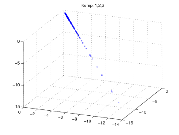
  Figure 5: Plot of the coefficients $c_{1},c_{2},c_{3}$

  The points $(c_{1}(m,p),c_{2}(m,p),c_{3}(m,p))$ seem to lie on a line in ${\mathbb{R}}^{3}$, which means that there should be two linear dependencies between the functions $c_{1},c_{2}$ and $c_{3}$. In order to identify these linear dependencies, we run the PSLQ algorithm [Ferguson and Bailey 1991, Ferguson, Bailey and Arno 1999] with the vectors $(c_{1},c_{2},1)$ as input (see Remark after the end of the proof, concerning implementation of this step). On this way we obtain the conjecture

  $$c_{1}-c_{2}=\epsilon^{2}(\omega_{1}-\omega_{2}).$$

  Similarly, running the PSLQ algorithm with the vectors $(c_{2},c_{3},1)$ as input leads to the conjecture

  $$c_{2}-c_{3}=\epsilon^{2}(\omega_{2}-\omega_{3}).$$

  Having identified (numerically!) these two linear relations, we use them instead of two equations in the system (39), say the equations for $i=1,2$. The resulting system becomes extremely simple:

  $$\left\{\begin{array}[]{l}c_{1}p_{1}^{2}+c_{2}p_{2}^{2}+c_{3}p_{3}^{2}=1,\\ c_{1}-c_{2}=\epsilon^{2}(\omega_{1}-\omega_{2}),\\ c_{2}-c_{3}=\epsilon^{2}(\omega_{2}-\omega_{3}).\end{array}\right.$$

  It contains no iterates of $f$ at all and can be solved immediately by hands, with the result (37). It should be stressed that this result still remains conjectural, and one has to prove a posteriori that the functions $c_{1},c_{2},c_{3}$ are integrals of motion.

• Alternatively, we can combine the above approach based on the prescription (E) with the recipe (D). For this, we use just one of the linear dependencies found above to replace the equation in (39) with $i=2$, and then let MAPLE solve the remaining system. The computation takes 22,33 secs. on a 1.83 Ghz Core Duo PC and consumes 32,43 MB RAM. The output is still as in (37), but arguing this way one does not need to verify a posteriori that $c_{1},c_{2},c_{3}$ are integrals of motion, because they are manifestly even functions of $\epsilon$, while the symmetry of the linear system with respect to $\epsilon$ has been broken.

To finish the proof along the lines of the first of the possible arguments above, we show how to verify the statement that the function $J$ in (38) is an integral of motion, i.e., that

$$\frac{p_{1}^{2}+p_{2}^{2}+p_{3}^{2}}{1-\epsilon^{2}(\omega_{1}p_{1}^{2}+\omega_{2}p_{2}^{2}+\omega_{3}p_{3}^{2})}=\frac{\widetilde{p}_{1}^{2}+\widetilde{p}_{2}^{2}+\widetilde{p}_{3}^{2}}{1-\epsilon^{2}(\omega_{1}\widetilde{p}_{1}^{2}+\omega_{2}\widetilde{p}_{2}^{2}+\omega_{3}\widetilde{p}_{3}^{2})}.$$

This is equivalent to

$$\widetilde{p}_{1}^{2}-p_{1}^{2}+\widetilde{p}_{2}^{2}-p_{2}^{2}+\widetilde{p}_{3}^{2}-p_{3}^{2}$$

$$= \epsilon^{2}\left[(\omega_{2}-\omega_{1})(\widetilde{p}_{1}^{2}p_{2}^{2}-\widetilde{p}_{2}^{2}p_{1}^{2})+(\omega_{3}-\omega_{2})(\widetilde{p}_{2}^{2}p_{3}^{2}-\widetilde{p}_{3}^{2}p_{2}^{2})+(\omega_{1}-\omega_{3})(\widetilde{p}_{3}^{2}p_{1}^{2}-\widetilde{p}_{1}^{2}p_{3}^{2})\right].$$

On the left-hand side of this equation we replace $\widetilde{p}_{i}-p_{i}$ through the expressions from the last three equations of motion (6.2), on the right-hand side we replace $\epsilon(\omega_{k}-\omega_{j})(\widetilde{p}_{j}p_{k}+p_{j}\widetilde{p}_{k})$ by $\widetilde{m}_{i}-m_{i}$, according to the first three equations of motion (6.2). This brings the equation we want to prove into the form

$$(\widetilde{p}_{1}+p_{1})(\widetilde{m}_{3}p_{2}+m_{3}\widetilde{p}_{2}-\widetilde{m}_{2}p_{3}-m_{2}\widetilde{p}_{3})\;+$$

$$(\widetilde{p}_{2}+p_{2})(\widetilde{m}_{1}p_{3}+m_{1}\widetilde{p}_{3}-\widetilde{m}_{3}p_{1}-m_{3}\widetilde{p}_{1})\;+$$

$$(\widetilde{p}_{3}+p_{3})(\widetilde{m}_{2}p_{1}+m_{2}\widetilde{p}_{1}-\widetilde{m}_{1}p_{2}-m_{1}\widetilde{p}_{2})\;=$$

$$=(\widetilde{p}_{1}p_{2}-p_{1}\widetilde{p}_{2})(\widetilde{m}_{3}-m_{3})+(\widetilde{p}_{2}p_{3}-p_{2}\widetilde{p}_{3})(\widetilde{m}_{1}-m_{1})+(\widetilde{p}_{3}p_{1}-p_{3}\widetilde{p}_{1})(\widetilde{m}_{2}-m_{2}).$$

But the latter equation is an algebraic identity in twelve variables $m_{k},p_{k},\widetilde{m}_{k},\widetilde{p}_{k}$. This finishes the proof. $\Box$

Remark

In the above proof and on many occasions below we make use of the PSLQ algorithm in order to identify possible linear relations among conserved quantities. Its applications are well documented in the literature on Experimental Mathematics [Borwein and Bailey 2003, Borwein, Bailey and Girgensohn 2004], so that we restrict ourselves here to a couple of minor remarks. We apply the PSLQ algorithm to the numerical values of (the candidates for) the conserved quantities obtained from the algorithm (N). We note that it is crucial to apply the PSLQ algorithm with many different initial data; from the large amount of possible linear relations one should, of course, filter out those relations which stay unaltered for different initial data. It proved useful to perform these computations with rational data (initial values of phase variables and parameters of the map) as well as with high precision floating point numbers. In our experiments we have been able to automate this task to a large extent. All computations of this kind were performed on an Apple MacBook with a 1.83 GHz Intel Core Duo processor and 2 GB of RAM.

6.5 Remaining HK-bases

We now consider the remaining HK-bases $\Phi_{1}$,$\Phi_{2}$ and $\Phi_{3}$. Here we are dealing with the three linear systems

$$(\alpha_{1}p_{1}^{2}+\alpha_{2}p_{2}^{2}+\alpha_{3}p_{3}^{2}+\alpha_{4}m_{1}^{2}+\alpha_{5}m_{2}^{2}+\alpha_{6}m_{3}^{2})\circ f^{i}(m,p) = m_{1}p_{1}\circ f^{i}(m,p),$$ (40)

$$(\beta_{1}p_{1}^{2}+\beta_{2}p_{2}^{2}+\beta_{3}p_{3}^{2}+\beta_{4}m_{1}^{2}+\beta_{5}m_{2}^{2}+\beta_{6}m_{3}^{2})\circ f^{i}(m,p) = m_{2}p_{2}\circ f^{i}(m,p),$$ (41)

$$(\gamma_{1}p_{1}^{2}+\gamma_{2}p_{2}^{2}+\gamma_{3}p_{3}^{2}+\gamma_{4}m_{1}^{2}+\gamma_{5}m_{2}^{2}+\gamma_{6}m_{3}^{2})\circ f^{i}(m,p) = m_{3}p_{3}\circ f^{i}(m,p),\qquad$$ (42)

already made non-homogeneous by normalizing the last coefficient in each system, as in recipe (B), with $l=7$. The claim about each of the systems is that it admits a unique solution for $i\in{\mathbb{Z}}$. It is enough to solve each system for two different but intersecting ranges of $l-1=6$ consecutive indices $i$, such as $i\in[-2,3]$ and $i\in[-3,2]$, and to show that solutions coincide for both ranges (recipe (C)). Actually, since the index range $i\in[-2,3]$ is non-symmetric, it would be enough to consider the system for this one range and to show that the solutions $\alpha_{j},\beta_{j},\gamma_{j}$ are even functions with respect to $\epsilon$ (recipe (D)). However, symbolic manipulations with the iterates $f^{i}$ for $i=\pm 2,\pm 3$ are impossible. In what follows, we will gradually extend the available information about the coefficients $\alpha_{j},\beta_{j},\gamma_{j}$, which at the end will allow us to get the analytic expressions for all of them and to prove that they are integrals, indeed.

6.6 First additional HK-basis

Theorem 11 shows that, after finding the HK-basis $\Phi_{0}$ with $\dim K_{\Phi_{0}}(x)=1$ it is enough to concentrate on (sub)-bases not containing the constant function $\varphi_{10}(m,p)=1$. It turns out to be possible to find a HK-basis without $\varphi_{10}$ and with a one-dimensional null-space, which is more amenable to a symbolic treatment than $\Phi_{1},\Phi_{2},\Phi_{3}$. Numerical algorithm (N) suggests that the following set of functions is a HK-basis with $d=1$:

$$\Psi=(p_{1}^{2},p_{2}^{2},p_{3}^{2},m_{1}p_{1},m_{2}p_{2},m_{3}p_{3}).$$ (43)

Theorem 13

The set (43) is a HK-basis for the map (31) with $\dim K_{\Psi}(m,p)=1$. At every point $(m,p)\in{\mathbb{R}}^{6}$ there holds:

$$K_{\Psi}(m,p)=[-1:-1:-1:d_{7}:d_{8}:d_{9}],$$

with

$$d_{k}=\frac{(p_{1}^{2}+p_{2}^{2}+p_{3}^{2})(1+\epsilon^{2}d_{k}^{(2)}+\epsilon^{4}d_{k}^{(4)}+\epsilon^{6}d_{k}^{(6)})}{\Delta}\,,\quad k=7,8,9,$$ (44)

$$\Delta=m_{1}p_{1}+m_{2}p_{2}+m_{3}p_{3}+\epsilon^{2}\Delta^{(4)}+\epsilon^{4}\Delta^{(6)}+\epsilon^{6}\Delta^{(8)},$$ (45)

where $d^{(2q)}_{k}$ and $\Delta^{(2q)}$ are homogeneous polynomials of degree $2q$ in phase variables. In particular,

$$d_{7}^{(2)} = m_{1}^{2}+m_{2}^{2}+m_{3}^{2}+(\omega_{2}+\omega_{3}-2\omega_{1})p_{1}^{2}+(\omega_{3}-\omega_{2})p_{2}^{2}+(\omega_{2}-\omega_{3})p_{3}^{2},$$

$$d_{8}^{(2)} = m_{1}^{2}+m_{2}^{2}+m_{3}^{2}+(\omega_{3}-\omega_{1})p_{1}^{2}+(\omega_{3}+\omega_{1}-2\omega_{2})p_{2}^{2}+(\omega_{1}-\omega_{3})p_{3}^{2},$$

$$d_{9}^{(2)} = m_{1}^{2}+m_{2}^{2}+m_{3}^{2}+(\omega_{2}-\omega_{1})p_{1}^{2}+(\omega_{1}-\omega_{2})p_{2}^{2}+(\omega_{1}+\omega_{2}-2\omega_{3})p_{3}^{2},\qquad$$

and

$$\Delta^{(4)}=m_{1}p_{1}d_{7}^{(2)}+m_{2}p_{2}d_{8}^{(2)}+m_{3}p_{3}d_{9}^{(2)}.$$

(All other polynomials are too messy to be given here.) The functions $d_{7},d_{8},d_{9}$ are integrals of the map (31). They are dependent due to the linear relation

$$(\omega_{2}-\omega_{3})d_{7}+(\omega_{3}-\omega_{1})d_{8}+(\omega_{1}-\omega_{2})d_{9}=0.$$ (46)

Any two of them are functionally independent. Moreover, any two of them together with $J$ are still functionally independent.

Proof. As already mentioned, numerical experiments suggest that for any $(m,p)\in{\mathbb{R}}^{6}$ there exists a one-dimensional space of vectors $(d_{1},d_{2},d_{3},d_{7},d_{8},d_{9})$ satisfying

$$(d_{1}p_{1}^{2}+d_{2}p_{2}^{2}+d_{3}p_{3}^{2}+d_{7}m_{1}p_{1}+d_{8}m_{2}p_{2}+d_{9}m_{3}p_{3})\circ f^{i}(m,p)=0$$

for $i=0,1,\ldots,5$. According to recipe (A), one can equally well consider this system for $i=-2,-1,\ldots,3$, which however still contains the third iterate of $f$ and is therefore not manageable. Therefore, we apply recipe (E) and look for linear relations between the (numerical) solutions. Two such relations can be observed immediately, namely

$$d_{1}=d_{2}=d_{3}.$$ (47)

Accepting these (still hypothetical) relations and applying recipe (B), i.e., setting the common value of (47) equal to $-1$, we arrive at the non-homogeneous system of only 3 linear relations

$$(d_{7}m_{1}p_{1}+d_{8}m_{2}p_{2}+d_{9}m_{3}p_{3})\circ f^{i}(m,p)=(p_{1}^{2}+p_{2}^{2}+p_{3}^{2})\circ f^{i}(m,p)$$ (48)

for $i=-1,0,1$. Fortunately, it is possible to find one more linear relation between $d_{7},d_{8},d_{9}$. This was discovered numerically: we produced a three-dimensional plot of the points $(d_{7}(m,p),d_{8}(m,p),d_{9}(m,p))$ which can be seen in Fig. 6 in two different projections.

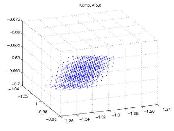
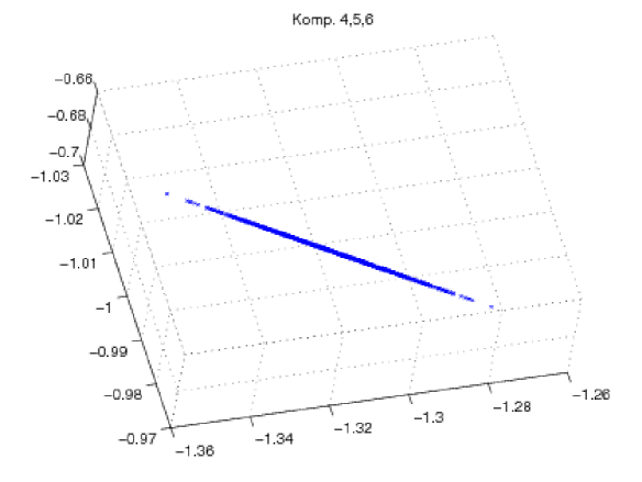
Figure 6: Plot of the points $(d_{7},d_{8},d_{9})$ for 729 values of $(m,p)$ from a six-dimensional grid around the point $(1,1,1,1,1,1)$ with a grid size of 0.01 and the parameters $\epsilon=0.1$, $\omega_{1}=0.1$, $\omega_{2}=0.2$, $\omega_{3}=0.3$.

This figure suggests that all these points lie on a plane in ${\mathbb{R}}^{3}$, the second picture being a “side view” along a direction parallel to this plane. Thus, it is plausible that one more linear relation exists. With the help of the PSLQ algorithm this hypothetic relation can be then identified as eq. (46). Now the ansatz (48) is reduced to the following system of three equations for $(d_{7},d_{8},d_{9})$, which involves only one iterate of the map $f$:

$$\left\{\begin{array}[]{l}(d_{7}m_{1}p_{1}+d_{8}m_{2}p_{2}+d_{9}m_{3}p_{3})\circ f^{i}(m,p)=(p_{1}^{2}+p_{2}^{2}+p_{3}^{2})\circ f^{i}(m,p),\quad i=0,1,\\ (\omega_{2}-\omega_{3})d_{7}+(\omega_{3}-\omega_{1})d_{8}+(\omega_{2}-\omega_{2})d_{9}=0.\end{array}\right.$$ (49)

This system can be solved by MAPLE, resulting in functions given in eqs. (44), (45). These (long) expressions can be found in [Worksheets]. They are manifestly even functions of $\epsilon$, while the system has no symmetry with respect to $\epsilon\mapsto-\epsilon$. This proves that they are integrals of motion for the map $f$. This argument slightly generalizes the recipes (D) and (E), and, since it is used not only here but also on several further occasions in this paper, we give here its formalization.

Proposition 14

Consider a map $f:{\mathbb{R}}^{6}\to{\mathbb{R}}^{6}$ depending on a parameter $\epsilon$, reversible in the sense of eq. (32). Let $I(m,p,\epsilon)$ be an integral of $f$, even in $\epsilon$, and let $A_{1},A_{2},A_{3}\in{\mathbb{R}}$. Suppose that the set of functions $\Phi=(\varphi_{1},\ldots,\varphi_{4})$ is such that the system of three linear equations for $(a_{1},a_{2},a_{3})$,

$$\left\{\begin{array}[]{l}(a_{1}\varphi_{1}+a_{2}\varphi_{2}+a_{3}\varphi_{3})\circ f^{i}(m,p,\epsilon)=\varphi_{4}\circ f^{i}(m,p,\epsilon),\quad i=0,1,\\ A_{1}a_{1}+A_{2}a_{2}+A_{3}a_{3}=I(m,p,\epsilon),\end{array}\right.$$ (50)

admits a unique solution which is even with respect to $\epsilon$. Then this solution $(a_{1},a_{2},a_{3})$ consists of integrals of the map $f$, and $\Phi$ is a HK-basis with $\dim K_{\Phi}(m,p)=1$.

Proof. Since $(a_{1},a_{2},a_{3})$ are even functions of $\epsilon$, they satisfy also the system (50) with $\epsilon\mapsto-\epsilon$, which, due to the reversibility (32), can be represented as

$$\left\{\begin{array}[]{l}(a_{1}\varphi_{1}+a_{2}\varphi_{2}+a_{3}\varphi_{3})\circ f^{i}(m,p,\epsilon)=\varphi_{4}\circ f^{i}(m,p,\epsilon),\quad i=0,-1,\\ A_{1}a_{1}+A_{2}a_{2}+A_{3}a_{3}=I(m,p,\epsilon).\end{array}\right.$$ (51)

Since the functions $(a_{1},a_{2},a_{3})$ are uniquely determined by any of the systems (50) or (51), we conclude that they remain invariant under the change $(m,p)\mapsto f(m,p,\epsilon)$, or, in other words, that they are integrals of motion. Finally, we can conclude that these functions satisfy equation $(a_{1}\varphi_{1}+a_{2}\varphi_{2}+a_{3}\varphi_{3})\circ f^{i}=\varphi_{4}\circ f^{i}$ for all $i\in{\mathbb{Z}}$ (and can be uniquely determined by this property), and that linear relation $A_{1}a_{1}+A_{2}a_{2}+A_{3}a_{3}=I$ is satisfied, as well. $\Box$

Application of Proposition 14 to system (49) shows that $d_{7},d_{8},d_{9}$ are integrals of motion, since they are even in $\epsilon$. Note that here, as always in similar context, the evenness of solutions is due to “miraculous cancellation” of the equal non-even polynomials which factor out both in the numerators and denominators of the solutions. In the present computation, these common non-even factors are of degree 2 in $\epsilon$.

It remains to prove that any two of the integrals $d_{7},d_{8},d_{9}$ together with the previously found integral $J$ are functionally independent. For this aim, we show that from such a triple of integrals one can construct another triple of integrals which yields in the limit $\epsilon\to 0$ three independent conserved quantities $H_{3},H_{4},H_{1}$ of the continuous Clebsch system. Indeed:

$$J = p_{1}^{2}+p_{2}^{2}+p_{3}^{2}+O(\epsilon^{2})=H_{3}+O(\epsilon^{2}),$$

$$\frac{J}{d_{k+6}} = m_{1}p_{1}+m_{2}p_{2}+m_{3}p_{3}+O(\epsilon^{2})=H_{4}+O(\epsilon^{2}).$$

On the other hand, it is easy to derive:

$$\frac{d_{7}}{d_{8}}=1+\epsilon^{2}(d_{7}^{(2)}-d_{8}^{(2)})+O(\epsilon^{4})=1+\epsilon^{2}(\omega_{2}-\omega_{1})(p_{1}^{2}+p_{2}^{2}+p_{3}^{2})+O(\epsilon^{4}),$$

and, taking this into account and computing the terms of order $\epsilon^{4}$, one finds:

$$\frac{d_{7}}{d_{8}}-1-\epsilon^{2}(\omega_{2}-\omega_{1})J=\epsilon^{4}(\omega_{2}-\omega_{1})(2H_{4}^{2}+\omega_{2}H_{3}^{2}-2H_{3}H_{1})+O(\epsilon^{6}),$$

from which one easily extracts $H_{1}$. This proves our claim. $\Box$

Remark

With the basis $\Psi$, we encounter for the first time the following interesting phenomenon: it can happen that a HK-basis with a one-dimensional null-space provides several (in this case two) functionally independent integrals. With Theorem 13, we established existence of three independent conserved quantities and two HK-bases with linearly independent null-spaces. So, every orbit of the discrete Clebsch system is shown to lie in a three-dimensional manifold which belongs to an intersection of two quadrics in ${\mathbb{R}}^{6}$. The aim of the following is to find one more independent integral and two more HK-bases with one-dimensional null-spaces linearly independent on $K_{\Phi_{0}}$, $K_{\Psi}$.

6.7 Second additional HK-basis

From the (still hypothetic) properties (40)–(42) of the bases $\Phi_{1},\Phi_{2},\Phi_{3}$ there follows that for any $(m,p)\in{\mathbb{R}}^{6}$ the system of linear equations

$$(g_{1}p_{1}^{2}+g_{2}p_{2}^{2}+g_{3}p_{3}^{2}+g_{4}m_{1}^{2}+g_{5}m_{2}^{2}+g_{6}m_{3}^{2})\circ f^{i}(m,p)=(m_{1}p_{1}+m_{2}p_{2}+m_{3}p_{3})\circ f^{i}(m,p)\;\;$$ (52)

has a unique solution $(g_{1},g_{2},g_{3},g_{4},g_{5},g_{6})$. Indeed, the solution should be given by

$$g_{j}=\alpha_{j}+\beta_{j}+\gamma_{j},\quad j=1,\ldots,6.$$ (53)

As for the bases $\Phi_{1},\Phi_{2},\Phi_{3}$, the solution of (52) can be determined by solving these equations for two different but intersecting ranges of 6 consecutive values of $i$, say for $i\in[-3,2]$ and $i\in[-2,3]$. However, it turns out that, due to the existence of several linear relations between the solutions $g_{j}$, system (52) is much easier to deal with than systems (40)–(42), so that the functions $g_{j}$ can be determined and studied independently of $\alpha_{j},\beta_{j},\gamma_{j}$.

Theorem 15

The set of functions

$$\Theta=(p_{1}^{2},p_{2}^{2},p_{3}^{2},m_{1}^{2},m_{2}^{2},m_{3}^{2},m_{1}p_{1}+m_{2}p_{2}+m_{3}p_{3})$$

is a HK-basis for the map (31) with $\dim K_{\Theta}(m,p)=1$. At every point $(m,p)\in{\mathbb{R}}^{6}$ there holds:

$$K_{\Theta}(m,p)=[g_{1}:g_{2}:g_{3}:g_{4}:g_{5}:g_{6}:-1].$$

Here $g_{1},g_{2},g_{3}$ are integrals of the map (31) given by

$$g_{k}=\frac{g_{k}^{(4)}+\epsilon^{2}g_{k}^{(6)}+\epsilon^{4}g_{k}^{(8)}+\epsilon^{6}g_{k}^{(10)}}{2(p_{1}^{2}+p_{2}^{2}+p_{3}^{2})\Delta}\,,\qquad k=1,2,3,$$

where $g_{k}^{(2q)}$ are homogeneous polynomials of degree $2q$ in phase variables, and $\Delta$ is given in eq. (45). For instance,

$$g_{k}^{(4)}=2H_{4}^{2}-H_{3}H_{1}+\omega_{k}H_{3}^{2}.$$

Integrals $g_{4},g_{5},g_{6}$ are given by

$$g_{4}=\frac{g_{2}-g_{3}}{\omega_{2}-\omega_{3}}\,,\quad g_{5}=\frac{g_{3}-g_{1}}{\omega_{3}-\omega_{1}}\,,\quad g_{6}=\frac{g_{1}-g_{2}}{\omega_{1}-\omega_{2}}\,.$$

Proof. Since system (52) involves too many iterates of $f$ for a symbolical treatment, we look for linear relations between the (numerical) solutions of this system. Application of the PSLQ algorithm allows us to identify three such relations, as given in eq. (15). This reduces system (52) to the following one:

$$\bigg{[}g_{1}\Big{(}p_{1}^{2}+\frac{m_{2}^{2}}{\omega_{1}-\omega_{3}}+\frac{m_{3}^{2}}{\omega_{1}-\omega_{2}}\Big{)}+g_{2}\Big{(}p_{2}^{2}+\frac{m_{1}^{2}}{\omega_{2}-\omega_{3}}+\frac{m_{3}^{2}}{\omega_{2}-\omega_{1}}\Big{)}$$

$$+g_{3}\Big{(}p_{3}^{2}+\frac{m_{1}^{2}}{\omega_{3}-\omega_{2}}+\frac{m_{2}^{2}}{\omega_{3}-\omega_{1}}\Big{)}\bigg{]}\circ f^{i}(m,p)=(m_{1}p_{1}+m_{2}p_{2}+m_{3}p_{3})\circ f^{i}(m,p).\qquad\quad$$ (54)

Thus, one can say that we are dealing with a reduced Hirota-Kimura basis consisting of $l=4$ functions

$$\widetilde{\Theta}=(I_{1},I_{2},I_{3},H_{4}),$$

see (6.1). Interestingly, this is a basis of integrals for the continuous-time Clebsch system, but we do not know whether this is just a coincidence or has some deeper meaning. System (6.7) has to be solved for two different but intersecting ranges of $l-1=3$ consecutive indices $i$. It would be enough to show that the solution for one non-symmetric range, e.g., for $i\in[0,2]$, consists of even functions of $\epsilon$. However, this non-symmetric system involves with necessity the second iterate $f^{2}$. To avoid dealing with $f^{2}$, one more linear relation for $g_{1},g_{2},g_{3}$ would be needed. Such a relation has been found with the help of PSLQ algorithm, it does not have constant coefficients anymore but involves the previously found integrals $d_{7},d_{8},d_{9}$:

$$(\omega_{2}-\omega_{3})g_{1}+(\omega_{3}-\omega_{1})g_{2}+(\omega_{1}-\omega_{2})g_{3}=\frac{1}{2}(\omega_{2}-\omega_{3})(\omega_{3}-\omega_{1})(d_{8}-d_{7}).$$ (55)

Of course, due to eq. (46), the right-hand side of eq. (55) can be equivalently put as

$$\frac{1}{2}(\omega_{3}-\omega_{1})(\omega_{1}-\omega_{2})(d_{9}-d_{8})=\frac{1}{2}(\omega_{1}-\omega_{2})(\omega_{2}-\omega_{3})(d_{7}-d_{9}).$$

The linear system consisting of eq. (6.7) for $i=0,1$ and eq. (55) can be solved by MAPLE with the result given in theorem. Since $(d_{7},d_{8},d_{9})$ are already proven to be integrals of motion, and since the solutions $(g_{1},g_{2},g_{3})$ are manifestly even in $\epsilon$, Proposition 14 yields that $(g_{1},g_{2},g_{3})$ are integrals of the map $f$. $\Box$

Theorem 15 gives us the third HK-basis with a one-dimensional null-space for the discrete Clebsch system. Thus, it shows that every orbit lies in the intersection of three quadrics in ${\mathbb{R}}^{6}$. What concerns the integrals of motion, it turns out that the basis $\Theta$ does not provide us with additional ones: a numerical check with gradients shows that integrals $g_{1},g_{2},g_{3}$ are functionally dependent from the previously found ones. At this point we are lacking one more HK-basis with a one-dimensional null-space, linearly independent from $K_{\Phi_{0}}$, $K_{\Psi}$, $K_{\Theta}$, and one more integral of motion, functionally independent from $J$ and $d_{7},d_{8}$.

6.8 Proof for the bases $\Phi_{1},\Phi_{2},\Phi_{3}$

Now we return to the bases $\Phi_{1},\Phi_{2},\Phi_{3}$ discussed in Sect. 6.5. In order to be able to solve systems (40)–(42) symbolically and to prove that the solutions $\alpha_{j},\beta_{j},\gamma_{j}$ are indeed integrals, we have to find additional linear relations for these quantities (recipe (E)). Within each set of coefficients we were able to identify just one relation:

$$(\omega_{1}-\omega_{3})\alpha_{5} = (\omega_{1}-\omega_{2})\alpha_{6},$$ (56)

$$(\omega_{2}-\omega_{3})\beta_{4} = (\omega_{2}-\omega_{1})\beta_{6},$$ (57)

$$(\omega_{3}-\omega_{2})\gamma_{4} = (\omega_{3}-\omega_{1})\gamma_{5}.$$ (58)

This reduces the number of equations in each system by one, which however does not resolve our problems. A way out consists in looking for linear relations among all the coefficients $\alpha_{j},\beta_{j},\gamma_{j}$. Remarkably, six more independent linear relations of this kind can be identified:

$$\alpha_{4}=\beta_{5}=\gamma_{6},$$ (59)

$$\frac{\alpha_{2}-\alpha_{3}-(\omega_{2}-\omega_{3})\alpha_{4}}{\omega_{2}-\omega_{3}}=\frac{\beta_{2}-\beta_{3}-(\omega_{2}-\omega_{3})\beta_{4}}{\omega_{3}-\omega_{1}}=\frac{\gamma_{2}-\gamma_{3}-(\omega_{2}-\omega_{3})\gamma_{4}}{\omega_{1}-\omega_{2}},\qquad$$ (60)

$$\frac{\alpha_{3}-\alpha_{1}-(\omega_{3}-\omega_{1})\alpha_{5}}{\omega_{2}-\omega_{3}}=\frac{\beta_{3}-\beta_{1}-(\omega_{3}-\omega_{1})\beta_{5}}{\omega_{3}-\omega_{1}}=\frac{\gamma_{3}-\gamma_{1}-(\omega_{3}-\omega_{1})\gamma_{5}}{\omega_{1}-\omega_{2}}.$$ (61)

There are two more similar relations:

$$\frac{\alpha_{1}-\alpha_{2}-(\omega_{1}-\omega_{2})\alpha_{6}}{\omega_{2}-\omega_{3}}=\frac{\beta_{1}-\beta_{2}-(\omega_{1}-\omega_{2})\beta_{6}}{\omega_{3}-\omega_{1}}=\frac{\gamma_{1}-\gamma_{2}-(\omega_{1}-\omega_{2})\gamma_{6}}{\omega_{1}-\omega_{2}},$$

but they follow from the already listed ones (56)–(61). We stress that all these linear relations were identified numerically, with the help of the PSLQ algorithm, and remain at this stage hypothetic.

With nine linear relations (56)–(61), we have to solve systems (40)–(42) simultaneously for a range of 3 consecutive indices $i$. Taking this range as $i=-1,0,1$ we can avoid dealing with $f^{2}$, which however would leave us with the problem of a proof that the solutions are integrals. Alternatively, we can choose the range $i=0,1,2$, and then the solutions are automatically integrals, as soon as it is established that they are even functions of $\epsilon$.

A symbolic solution of the system consisting of 18 linear equations, namely eqs. (40)–(42) with $i=0,1,2$ along with nine simple equations (56)–(61), would require astronomical amounts of memory, because of the complexity of $f^{2}$. However, this task becomes manageable and even simple for fixed (numerical) values of the phase variables $(m,p)$ and of the parameters $\omega_{i}$, while leaving $\epsilon$ a symbolic variable. For rational values of $m_{k},p_{k},\omega_{k}$ all computations can be done precisely (in rational arithmetic). This means that $\alpha_{j}$, $\beta_{j}$, and $\gamma_{j}$ can be evaluated, as functions of $\epsilon$, at arbitrary points in ${\mathbb{Q}}^{9}(m,p,\omega_{1},\omega_{2},\omega_{3})$. A big number of such evaluations provides us with a convincing evidence in favor of the claim that these functions are even in $\epsilon$.

In order to obtain a rigorous proof without dealing with $f^{2}$, further linear relations would be necessary. Before introducing these, we present some preliminary considerations. Assuming that $\Phi_{1},\Phi_{2},\Phi_{3}$ are HK-bases with one-dimensional null-spaces, results of Theorem 13 on the HK-basis $\Psi$ tell us that the row vector $(d_{7},d_{8},d_{9})$ is the unique left null-vector for the matrix

$$M_{2}=\begin{pmatrix}\alpha_{4}&\alpha_{5}&\alpha_{6}\\ \beta_{4}&\beta_{5}&\beta_{6}\\ \gamma_{4}&\gamma_{5}&\gamma_{6}\end{pmatrix},$$

normalized so that

$$(d_{7},d_{8},d_{9})M_{1}=(1,1,1),\quad{\rm where}\quad M_{1}=\begin{pmatrix}\alpha_{1}&\alpha_{2}&\alpha_{3}\\ \beta_{1}&\beta_{2}&\beta_{3}\\ \gamma_{1}&\gamma_{2}&\gamma_{3}\end{pmatrix}.$$

Note that due to eqs. (56)–(59) the matrix $M_{2}$ has at most four (linearly) independent entries. Denoting the common values in these equations by $A,B,C,D$, respectively, we find:

$$M_{2}=\begin{pmatrix}\alpha_{4}&\alpha_{5}&\alpha_{6}\\ \beta_{4}&\beta_{5}&\beta_{6}\\ \gamma_{4}&\gamma_{5}&\gamma_{6}\end{pmatrix}=\begin{pmatrix}D&A/(\omega_{1}-\omega_{3})&A/(\omega_{1}-\omega_{2})\\ B/(\omega_{2}-\omega_{3})&D&B/(\omega_{2}-\omega_{1})\\ C/(\omega_{3}-\omega_{2})&C/(\omega_{3}-\omega_{1})&D\end{pmatrix}.$$ (62)

The existence of the left null-vector $(d_{7},d_{8},d_{9})$ shows that $\det(M_{2})=0$, or, equivalently,

$$D^{2}-\frac{AB}{(\omega_{1}-\omega_{3})(\omega_{2}-\omega_{3})}-\frac{BC}{(\omega_{2}-\omega_{1})(\omega_{3}-\omega_{1})}-\frac{CA}{(\omega_{3}-\omega_{2})(\omega_{1}-\omega_{2})}=0.$$ (63)

From eqs. (62) and (63) one easily derives that the row

$$\left(D-\frac{B}{\omega_{2}-\omega_{3}}-\frac{C}{\omega_{3}-\omega_{2}}\,,\,D-\frac{A}{\omega_{1}-\omega_{3}}-\frac{C}{\omega_{3}-\omega_{1}}\,,\,D-\frac{A}{\omega_{1}-\omega_{2}}-\frac{B}{\omega_{2}-\omega_{1}}\right)$$

$$\qquad=(\alpha_{4}-\beta_{4}-\gamma_{4},\,-\alpha_{5}+\beta_{5}-\gamma_{5},\,-\alpha_{6}-\beta_{6}+\gamma_{6})$$

is a left null-vector of the matrix $M_{2}$, and therefore $(d_{7},d_{8},d_{9})$ is proportional to this vector. The proportionality coefficient can be now determined with the help of the PSLQ algorithm and turns out to be extremely simple. Namely, the following relations hold:

$$\alpha_{4}-\beta_{4}-\gamma_{4} = D-\frac{B-C}{\omega_{2}-\omega_{3}}\;=\;\frac{1}{2}\,d_{7},$$ (64)

$$-\alpha_{5}+\beta_{5}-\gamma_{5} = D-\frac{C-A}{\omega_{3}-\omega_{1}}\;=\;\frac{1}{2}\,d_{8},$$ (65)

$$-\alpha_{6}-\beta_{6}+\gamma_{6} = D-\frac{A-B}{\omega_{1}-\omega_{2}}\;=\;\frac{1}{2}\,d_{9}.$$ (66)

Only two of them are independent, because of eq. (46). We note also that, according to eq. (53), one has

$$\alpha_{4}+\beta_{4}+\gamma_{4} = D+\frac{B-C}{\omega_{2}-\omega_{3}}\;=\;g_{4},$$ (67)

$$\alpha_{5}+\beta_{5}+\gamma_{5} = D+\frac{C-A}{\omega_{3}-\omega_{1}}\;=\;g_{5},$$ (68)

$$\alpha_{6}+\beta_{6}+\gamma_{6} = D+\frac{A-B}{\omega_{1}-\omega_{2}}\;=\;g_{6}.$$ (69)

Equations (64)–(69) and (63) are already enough to determine all four integrals $A,B,C,D$, that is, all $\alpha_{j},\beta_{j},\gamma_{j}$ with $j=4,5,6$, provided it is proven that they are indeed integrals. These (conditional) results read:

$$A = \frac{1+\epsilon^{2}A^{(2)}+\epsilon^{4}A^{(4)}+\epsilon^{6}A^{(6)}+\epsilon^{8}A^{(8)}}{2\epsilon^{2}\Delta}\,,$$ (70)

$$B = \frac{1+\epsilon^{2}B^{(2)}+\epsilon^{4}B^{(4)}+\epsilon^{6}B^{(6)}+\epsilon^{8}B^{(8)}}{2\epsilon^{2}\Delta}\,,$$ (71)

$$C = \frac{1+\epsilon^{2}C^{(2)}+\epsilon^{4}C^{(4)}+\epsilon^{6}C^{(6)}+\epsilon^{8}C^{(8)}}{2\epsilon^{2}\Delta}\,,$$ (72)

$$D = \frac{p_{1}^{2}+p_{2}^{2}+p_{3}^{2}+\epsilon^{2}D^{(4)}+\epsilon^{4}D^{(6)}+\epsilon^{6}D^{(8)}}{2\Delta}\,,$$ (73)

where $A^{(2q)}$, $B^{(2q)}$, $C^{(2q)}$, $D^{(2q)}$ are homogeneous polynomials of degree $2q$ in phase variables, for instance,

$$A^{(2)} = B^{(2)}\;=\;C^{(2)}$$

$$= m_{1}^{2}+m_{2}^{2}+m_{3}^{2}+(\omega_{2}+\omega_{3}-2\omega_{1})p_{1}^{2}+(\omega_{3}+\omega_{1}-2\omega_{2})p_{2}^{2}+(\omega_{1}+\omega_{2}-2\omega_{3})p_{3}^{2},$$

$$D^{(4)} = (m_{1}p_{1}+m_{2}p_{2}+m_{3}p_{3})^{2}$$

$$+(p_{1}^{2}+p_{2}^{2}+p_{3}^{2})\Big{(}(\omega_{2}+\omega_{3}-2\omega_{1})p_{1}^{2}+(\omega_{3}+\omega_{1}-2\omega_{2})p_{2}^{2}+(\omega_{1}+\omega_{2}-2\omega_{3})p_{3}^{2}\Big{)}.$$

We remark that eq. (63) tells us that no more than three of the functions $A,B,C,D$ are actually functionally independent. Computation with gradients shows that $A,B,C$ are functionally independent, indeed. Moreover, all other previously found integrals $J$, $d_{7},d_{8},d_{9}$, and $g_{1},g_{2},g_{3}$ are functionally dependent on these ones.

Theorem 16

The sets (34)–(36) are HK-bases for the map (31) with $\dim K_{\Phi_{1}}(m,p)=\dim K_{\Phi_{2}}(m,p)=\dim K_{\Phi_{3}}(m,p)=1$. At each point $(m,p)\in{\mathbb{R}}^{6}$ there holds:

$$K_{\Phi_{1}}(m,p) = [\alpha_{1}:\alpha_{2}:\alpha_{3}:\alpha_{4}:\alpha_{5}:\alpha_{6}:-1],$$

$$K_{\Phi_{2}}(m,p) = [\beta_{1}:\beta_{2}:\beta_{3}:\beta_{4}:\beta_{5}:\beta_{6}:-1],$$

$$K_{\Phi_{3}}(m,p) = [\gamma_{1}:\gamma_{2}:\gamma_{3}:\gamma_{4}:\gamma_{5}:\gamma_{6}:-1],$$

where $\alpha_{j}$,$\beta_{j}$, and $\gamma_{j}$ are rational functions of $(m,p)$, even with respect to $\epsilon$. They are integrals of motion for the map (31) and satisfy linear relations (56)–(61). For $j=4,5,6$ they are given by eqs. (62), (72), (73). For $j=1,2,3$ they are of the form

$$h=\frac{h^{(2)}+\epsilon^{2}h^{(4)}+\epsilon^{4}h^{(6)}+\epsilon^{6}h^{(8)}+\epsilon^{8}h^{(10)}+\epsilon^{10}h^{(12)}}{2\epsilon^{2}(p_{1}^{2}+p_{2}^{2}+p_{3}^{2})\Delta}\,,$$ (74)

where $h$ stands for any of the functions $\alpha_{j},\beta_{j},\gamma_{j}$, $j=1,2,3$, and the corresponding $h^{(2q)}$ are homogeneous polynomials in phase variables of degree $2q$. For instance,

$$\begin{array}[]{lll}\alpha_{1}^{(2)}=H_{3}-I_{1},&\alpha_{2}^{(2)}=-I_{1},&\alpha_{3}^{(2)}=-I_{1},\\ \beta_{1}^{(2)}=-I_{2},&\beta_{2}^{(2)}=H_{3}-I_{2},&\beta_{3}^{(2)}=-I_{2},\\ \gamma_{1}^{(2)}=-I_{3},&\gamma_{2}^{(2)}=-I_{3},&\gamma_{3}^{(2)}=H_{3}-I_{3}.\end{array}$$ (75)

The four functions $J$, $\alpha_{1}$, $\beta_{1}$ and $\gamma_{1}$ are functionally independent.

Proof. The proof consists of several steps.

Step 1. Consider the system for 18 unknowns $\alpha_{j},\beta_{j},\gamma_{j}$, $j=1,\ldots,6$, consisting of 17 linear equations: eqs. (40)–(42) with $i=0,1$, eqs. (56)–(61), and eqs. (64), (65). This system is underdetermined, so that in principle it admits a one-parameter family of solutions. Remarkably, the symbolic MAPLE solution shows that all variables $\alpha_{j},\beta_{j},\gamma_{j}$ with $j=4,5,6$ are determined by this system uniquely, the results coinciding with eqs. (62), (72)–(73). (Actually, the MAPLE answers are much more complicated, and their simplification has been performed with SINGULAR, which was used to cancel out common factors from the huge expressions in numerators and denominators of these rational functions.) Since these uniquely determined $\alpha_{j},\beta_{j},\gamma_{j}$ with $j=4,5,6$ are even functions of $\epsilon$, this proves that they (i.e., $A,B,C,D$) are integrals of motion.

Step 2. Having determined $\alpha_{j},\beta_{j},\gamma_{j}$ with $j=4,5,6$, we are in a position to compute $\alpha_{j},\beta_{j},\gamma_{j}$ with $j=1,2,3$. For instance, to obtain the values of $\alpha_{j}$ with $j=1,2,3$, we consider the symmetric linear system (40) with $i=-1,0,1$ (and with already found $\alpha_{4},\alpha_{5},\alpha_{6}$). This system has been solved by MAPLE. The solutions are huge rational functions which however turn out to admit massive cancellations. These cancellations have been performed with the help of SINGULAR. The resulting expressions for $\alpha_{1},\alpha_{2},\alpha_{3}$ turn out to satisfy the ansatz (74) with the leading terms given in the first line of eq. (75). (All further terms can be found in [Worksheets].) However, this computation does not prove that the functions so obtained are indeed integrals of motion. To prove this, one could, in principle, either check directly the identities $\alpha_{j}\circ f=\alpha_{j}$, $j=1,2,3$, or verify equation (40) with $i=2$. Both ways are prohibitively expensive, so that we have to look for an alternative one.

Step 3. The results of Step 2 yield an explicit expression for the function

$$F=(\omega_{2}-\omega_{3})\alpha_{1}+(\omega_{3}-\omega_{1})\alpha_{2}+(\omega_{1}-\omega_{2})\alpha_{3},$$ (76)

which is of the form

$$F=\frac{(\omega_{2}-\omega_{3})(1+\epsilon^{2}F^{(2)}+\epsilon^{4}F^{(4)}+\epsilon^{6}F^{(6)}+\epsilon^{8}F^{(8)})}{2\epsilon^{2}\Delta}.$$

It is of a crucial importance for our purposes that it can be proven directly that $F$ is an integral of motion. We have proved this with the method (G) based on the Gröbner basis for the ideal generated by discrete equations of motion. The application of this method to $F$ is more feasible that to any single of $\alpha_{j}$, $j=1,2,3$, because of the cancellation of the huge polynomial coefficient of $\epsilon^{10}$ in the numerator of $F$. Actually, more is true: $F$ is not only an integral, but is functionally dependent on the previously found ones, say on $J,d_{7},d_{8}$. For a proof of this claim, it would be most favorable to find the explicit dependence $F=F(J,d_{7},d_{8})$, but it remains unknown to us. Instead, we have chosen the way of verification that

$$\nabla F\in{\rm span}(\nabla J,\nabla d_{7},\nabla d_{8}).$$

This is easily checked numerically for arbitrarily many (rational) values of the data involved. For a symbolic check, one has to prove the existence of three scalar functions $\lambda_{1},\lambda_{2},\lambda_{3}$ such that

$$\nabla F=\lambda_{1}\nabla J+\lambda_{2}\nabla d_{7}+\lambda_{3}\nabla d_{8}.$$

This is the system of six equations for three unknowns. Since $J$ does not depend on $m_{k}$, one can determine $\lambda_{2}$, $\lambda_{3}$ from a system of only three equations:

$$\nabla_{m}F=\lambda_{2}\nabla_{m}d_{7}+\lambda_{3}\nabla_{m}d_{8}.$$

After that, it remains to check that $\nabla_{p}F-\lambda_{2}\nabla_{p}d_{7}-\lambda_{3}\nabla_{p}d_{8}$ is proportional to $\nabla_{p}J$. Clearly, these computations can be arranged so as to verify vanishing of certain (very big) polynomials. We have been able to perform these computations with the help of SINGULAR for symbolic $m_{k},p_{k}$ but with (several sets of) numeric values of coefficients $\omega_{k}$ only.

Step 4. The result of Step 3 allows us to proceed as follows. Consider the system of three linear equations for $\alpha_{1},\alpha_{2},\alpha_{3}$, consisting of (40) with $i=0,1$, and of

$$(\omega_{2}-\omega_{3})\alpha_{1}+(\omega_{3}-\omega_{1})\alpha_{2}+(\omega_{1}-\omega_{2})\alpha_{3}=F,$$

where $F$ is the explicit expression obtained and proven to be an integral on Step 3. This system can now be solved by MAPLE; the results, again simplified with SINGULAR, are even functions of $\epsilon$ (actually, the same ones obtained on Step 1 from the symmetric system). Non-even polynomials in $\epsilon$ of degree 7 cancel in a miraculous way from the numerators and the denominator. Now Proposition 14 assures that these solutions are integrals of motion.

Step 5. Finally, in order to find $\beta_{1},\beta_{2},\beta_{3}$ and $\gamma_{1},\gamma_{2},\gamma_{3}$, we solve the two systems consisting of (41), resp. (42) with $i=0,1$, and the first, resp. the second linear relation in eq. (60). The results are even functions of $\epsilon$, satisfying the ansatz (74) with the leading terms given in eq. (75). Proposition 14 yields that also these functions are integrals of motion. $\Box$

MAPLE worksheets for all computations used in this section can be found in [Worksheets].

6.9 Preliminary results on the Hirota-Kimura-type discretization of the general flow of the Clebsch system

The general flow of the Clebsch system, depending on three real parameters $b_{1},b_{2},b_{3}$ (or, rather, on their differences $b_{i}-b_{j}$, which gives two independent real parameters), reads as follows:

$$\left\{\begin{array}[]{l}\dot{m}=m\times Cm+p\times Bp\,,\vspace{.2truecm}\\ \dot{p}=p\times Cm,\end{array}\right.$$ (77)

where $B={\rm{diag}}(b_{1},b_{2},b_{3})$ and $C={\rm{diag}}(c_{1},c_{2},c_{3})$ with

$$c_{1}=\frac{b_{2}-b_{3}}{\omega_{2}-\omega_{3}}\,,\quad c_{2}=\frac{b_{3}-b_{1}}{\omega_{3}-\omega_{1}}\,,\quad c_{3}=\frac{b_{1}-b_{2}}{\omega_{1}-\omega_{2}}\,.$$ (78)

This flow is Hamiltonian with the quadratic Hamilton function

$$H=\frac{1}{2}\,\langle m,Cm\rangle+\frac{1}{2}\,\langle p,Bp\rangle=\frac{1}{2}\sum_{k=1}^{3}(c_{k}m_{k}^{2}+b_{k}p_{k}^{2})=\frac{1}{2}(b_{1}I_{1}+b_{2}I_{2}+b_{3}I_{3}).$$

In components eqs. (77) read:

$$\dot{m}_{1} = (c_{3}-c_{2})m_{2}m_{3}+(b_{3}-b_{2})p_{2}p_{3},$$

$$\dot{m}_{2} = (c_{1}-c_{3})m_{3}m_{1}+(b_{1}-b_{3})p_{3}p_{1},$$

$$\dot{m}_{3} = (c_{2}-c_{1})m_{1}m_{2}+(b_{2}-b_{1})p_{1}p_{2}.$$

$$\dot{p}_{1} = c_{3}m_{3}p_{2}-c_{2}m_{2}p_{3},$$

$$\dot{p}_{2} = c_{1}m_{1}p_{3}-c_{3}m_{3}p_{1},$$

$$\dot{p}_{3} = c_{2}m_{2}p_{1}-c_{1}m_{1}p_{2}.$$

The KH discretization of the flow (77) reads

$$\left\{\begin{array}[]{rcl}\widetilde{m}-m&=&\epsilon(\widetilde{m}\times Cm+m\times C\widetilde{m}+\widetilde{p}\times Bp+p\times B\widetilde{p}\,),\vspace{.2truecm}\\ \widetilde{p}-p&=&\epsilon\left(\widetilde{p}\times Cm+p\times C\widetilde{m}\right).\end{array}\right.$$

In components:

$$\widetilde{m}_{1}-m_{1} = \epsilon(c_{3}-c_{2})(\widetilde{m}_{2}m_{3}+m_{2}\widetilde{m}_{3})+\epsilon(b_{3}-b_{2})(\widetilde{p}_{2}p_{3}+p_{2}\widetilde{p}_{3}),$$

$$\widetilde{m}_{2}-m_{2} = \epsilon(c_{1}-c_{3})(\widetilde{m}_{3}m_{1}+m_{3}\widetilde{m}_{1})+\epsilon(b_{1}-b_{3})(\widetilde{p}_{3}p_{1}+p_{3}\widetilde{p}_{1}),$$

$$\widetilde{m}_{3}-m_{3} = \epsilon(c_{2}-c_{1})(\widetilde{m}_{1}m_{2}+m_{1}\widetilde{m}_{2})+\epsilon(b_{2}-b_{1})(\widetilde{p}_{1}p_{2}+p_{1}\widetilde{p}_{2}),$$

$$\widetilde{p}_{1}-p_{1} = \epsilon c_{3}(\widetilde{m}_{3}p_{2}+m_{3}\widetilde{p}_{2})-\epsilon c_{2}(\widetilde{m}_{2}p_{3}+m_{2}\widetilde{p}_{3}),$$

$$\widetilde{p}_{2}-p_{2} = \epsilon c_{1}(\widetilde{m}_{1}p_{3}+m_{1}\widetilde{p}_{3})-\epsilon c_{3}(\widetilde{m}_{3}p_{1}+m_{3}\widetilde{p}_{1}),$$

$$\widetilde{p}_{3}-p_{3} = \epsilon c_{2}(\widetilde{m}_{2}p_{1}+m_{2}\widetilde{p}_{1})-\epsilon c_{1}(\widetilde{m}_{1}p_{2}+m_{1}\widetilde{p}_{2}).$$ (79)

In what follows, we will use the abbreviations $b_{ij}=b_{i}-b_{j}$ and $c_{ij}=c_{i}-c_{j}$. The linear system (6.9) defines an explicit, birational map $f:{\mathbb{R}}^{6}\rightarrow{\mathbb{R}}^{6}$,

$$\begin{pmatrix}\widetilde{m}\\ \widetilde{p}\end{pmatrix}=f(m,p,\epsilon)=M^{-1}(m,p,\epsilon)\begin{pmatrix}m\\ p\end{pmatrix},$$ (80)

where

$$M(m,p,\epsilon)=\begin{pmatrix}1&\epsilon c_{23}m_{3}&\epsilon c_{23}m_{2}&0&\epsilon b_{23}p_{3}&\epsilon b_{23}p_{2}\\ \epsilon c_{31}m_{3}&1&\epsilon c_{31}m_{1}&\epsilon b_{31}p_{3}&0&\epsilon b_{31}p_{1}\\ \epsilon c_{12}m_{2}&\epsilon c_{12}m_{1}&1&\epsilon b_{12}p_{2}&\epsilon b_{12}p_{1}&0\\ 0&\epsilon c_{2}p_{3}&-\epsilon c_{3}p_{2}&1&-\epsilon c_{3}m_{3}&\epsilon c_{2}m_{2}\\ -\epsilon c_{1}p_{3}&0&\epsilon c_{3}p_{1}&\epsilon c_{3}m_{3}&1&-\epsilon c_{1}m_{1}\\ \epsilon c_{1}p_{2}&-\epsilon c_{2}p_{1}&0&-\epsilon c_{2}m_{2}&\epsilon c_{1}m_{1}&1\\ \end{pmatrix}.$$

As usual, map (80) possesses the reversibility property

$$f^{-1}(m,p,\epsilon)=f(m,p,-\epsilon).$$

Conjecture 17

All claims of Theorems 10, 11 hold also for the discretization (80) of the general flow of the Clebsch system, with the HK-basis $\Phi_{0}$ being replaced by

$$\Phi_{0}=(p_{1}^{2},p_{2}^{2},p_{3}^{2},m_{1}^{2},m_{2}^{2},m_{3}^{2},1).$$ (81)

This conjecture is supported by numerical results based on the algorithm (N). The claim concerning the set $\Phi_{0}$ given in eq. (81) is proven symbolically. In order to keep the notations compact, we give here this proof for the second flow of the Clebsch system only.

Recall that the first flow of the Clebsch system, considered in Sect. 6, corresponds to $b_{i}=\omega_{i}$ and $c_{i}=1$. The second flow is characterized by the Hamilton function

$$H=\frac{1}{2}H_{2}=\frac{1}{2}(\omega_{1}m_{1}^{2}+\omega_{2}m_{2}^{2}+\omega_{3}m_{3}^{2}-\omega_{2}\omega_{3}p_{1}^{2}-\omega_{1}\omega_{3}p_{2}^{2}-\omega_{1}\omega_{2}p_{3}^{2}).$$

In other words, the choice of parameters $b_{k}$ characterizing the second flow is

$$b_{1}=-\omega_{2}\omega_{3},\quad b_{2}=-\omega_{3}\omega_{1},\quad b_{3}=-\omega_{1}\omega_{2},$$ (82)

so that

$$c_{1}=\omega_{1},\quad c_{2}=\omega_{2},\quad c_{3}=\omega_{3}.$$ (83)

For the HK discretization of the second Clebsch flow, we give a more concrete formulation of our findings concerning the HK-basis $\Phi_{0}$, including a “nice” integral.

Theorem 18

For the map (80) the set of functions (81) is a HK-basis with $\dim K_{\Phi_{0}}(m,p)=1$. At each point $(m,p)\in{\mathbb{R}}^{6}$ there holds:

$$K_{\Phi_{0}}(m,p)=[e_{1}:e_{2}:e_{3}:e_{4}:e_{5}:e_{6}:-1],$$

where all $e_{i}$ are fractional-linear functions of a single integral $L=L(m,p,\epsilon)$ of the map (80) which is a quotient of two quadratic polynomials in $m_{k},p_{k}$.

If the coefficients $b_{k},c_{k}$ are as in eqs. (82), (83), then the integral $L$ can be taken as

$$L=\frac{E_{1}(\omega_{1}m_{1}^{2}+\omega_{2}\omega_{3}p_{1}^{2})+E_{2}(\omega_{2}m_{2}^{2}+\omega_{3}\omega_{1}p_{2}^{2})+E_{3}(\omega_{3}m_{3}^{2}+\omega_{1}\omega_{2}p_{3}^{2})}{1+\epsilon^{2}\omega_{1}(\omega_{1}m_{1}^{2}+\omega_{2}\omega_{3}p_{1}^{2})+\epsilon^{2}\omega_{2}(\omega_{2}m_{2}^{2}+\omega_{3}\omega_{1}p_{2}^{2})+\epsilon^{2}\omega_{3}(\omega_{3}m_{3}^{2}+\omega_{1}\omega_{2}p_{3}^{2})}\,,$$

with

$$E_{1}=\omega_{3}\omega_{1}+\omega_{1}\omega_{2}-\omega_{2}\omega_{3},\quad E_{2}=\omega_{1}\omega_{2}+\omega_{2}\omega_{3}-\omega_{3}\omega_{1},\quad E_{3}=\omega_{2}\omega_{3}+\omega_{3}\omega_{1}-\omega_{1}\omega_{2}.$$ (84)

In this case there holds:

$$\frac{e_{1}}{\omega_{2}\omega_{3}}=\frac{e_{4}}{\omega_{1}} = \frac{E_{1}}{L}-\epsilon^{2}\omega_{1}$$

$$= \frac{E_{1}+\epsilon^{2}(\omega_{1}-\omega_{2})E_{3}(\omega_{2}m_{2}^{2}+\omega_{3}\omega_{1}p_{2}^{2})+\epsilon^{2}(\omega_{1}-\omega_{3})E_{2}(\omega_{3}m_{3}^{2}+\omega_{1}\omega_{2}p_{3}^{2})}{E_{1}(\omega_{1}m_{1}^{2}+\omega_{2}\omega_{3}p_{1}^{2})+E_{2}(\omega_{2}m_{2}^{2}+\omega_{3}\omega_{1}p_{2}^{2})+E_{3}(\omega_{3}m_{3}^{2}+\omega_{1}\omega_{2}p_{3}^{2})},$$

$$\frac{e_{2}}{\omega_{3}\omega_{1}}=\frac{e_{5}}{\omega_{2}} = \frac{E_{2}}{L}-\epsilon^{2}\omega_{2}$$

$$= \frac{E_{2}+\epsilon^{2}(\omega_{2}-\omega_{3})E_{1}(\omega_{3}m_{3}^{2}+\omega_{1}\omega_{2}p_{3}^{2})+\epsilon^{2}(\omega_{2}-\omega_{1})E_{3}(\omega_{1}m_{1}^{2}+\omega_{2}\omega_{3}p_{1}^{2})}{E_{1}(\omega_{1}m_{1}^{2}+\omega_{2}\omega_{3}p_{1}^{2})+E_{2}(\omega_{2}m_{2}^{2}+\omega_{3}\omega_{1}p_{2}^{2})+E_{3}(\omega_{3}m_{3}^{2}+\omega_{1}\omega_{2}p_{3}^{2})},$$

$$\frac{e_{3}}{\omega_{1}\omega_{2}}=\frac{e_{6}}{\omega_{3}} = \frac{E_{3}}{L}-\epsilon^{2}\omega_{3}$$

$$= \frac{E_{3}+\epsilon^{2}(\omega_{3}-\omega_{1})E_{2}(\omega_{1}m_{1}^{2}+\omega_{2}\omega_{3}p_{1}^{2})+\epsilon^{2}(\omega_{3}-\omega_{2})E_{1}(\omega_{2}m_{2}^{2}+\omega_{3}\omega_{1}p_{2}^{2})}{E_{1}(\omega_{1}m_{1}^{2}+\omega_{2}\omega_{3}p_{1}^{2})+E_{2}(\omega_{2}m_{2}^{2}+\omega_{3}\omega_{1}p_{2}^{2})+E_{3}(\omega_{3}m_{3}^{2}+\omega_{1}\omega_{2}p_{3}^{2})}.$$

The numerator of $L$,

$$L(m,p,0)=E_{1}(\omega_{1}m_{1}^{2}+\omega_{2}\omega_{3}p_{1}^{2})+E_{2}(\omega_{2}m_{2}^{2}+\omega_{3}\omega_{1}p_{2}^{2})+E_{3}(\omega_{3}m_{3}^{2}+\omega_{1}\omega_{2}p_{3}^{2}),$$

is a linear combination of quadratic integrals of motion of the continuous Clebsch system.

Proof. We will only present the proof for the second Clebsch flow. The claim of the theorem refers to the linear system

$$(e_{1}p_{1}^{2}+e_{2}p_{2}^{2}+e_{3}p_{3}^{2}+e_{4}m_{1}^{2}+e_{5}m_{2}^{2}+e_{6}m_{3}^{2})\circ f^{i}(m,p)=1$$

for $i$ from the ranges containing 6 consecutive numbers, such as $i\in[-2,3]$ or $i\in[-3,2]$. As the solution of such a system clearly requires more iterates of the map $f$ than could be handled symbolically, we follow recipe (E) and look for linear relations between $e_{i}$. It turns out to be possible to identify the following five relations:

$$\omega_{1}e_{1}-\omega_{2}\omega_{3}e_{4} = 0,$$ (85)

$$\omega_{2}e_{2}-\omega_{3}\omega_{1}e_{5} = 0,$$ (86)

$$\omega_{3}e_{3}-\omega_{1}\omega_{2}e_{6} = 0,$$ (87)

$$e_{1}-e_{2}-(\omega_{1}-\omega_{2})e_{6} = \epsilon^{2}\omega_{3}^{2}(\omega_{1}-\omega_{2}),$$ (88)

$$e_{3}-e_{1}-(\omega_{3}-\omega_{1})e_{5} = \epsilon^{2}\omega_{2}^{2}(\omega_{3}-\omega_{1}).$$ (89)

Of course, there holds also a third non-homogeneous relation:

$$e_{2}-e_{3}-(\omega_{2}-\omega_{3})e_{4}=\epsilon^{2}\omega_{1}^{2}(\omega_{2}-\omega_{3}),$$

but actually it is a consequence of the previous five. As usual, these (at this point conjectural) identities can be (and have been) found using the PSLQ algorithm. Now we obtain the six functions $e_{i}$ by solving a simple system of six linear equations which involves no iterates of the map $f$ at all and consists of

$$e_{1}p_{1}^{2}+e_{2}p_{2}^{2}+e_{3}p_{3}^{2}+e_{4}m_{1}^{2}+e_{5}m_{2}^{2}+e_{6}m_{3}^{2}=1\,$$

along with the relations (85)–(89). The solution is given in the formulation of the theorem. To prove that the function $L$ is an integral of motion one can use a straightforward computation using MAPLE. Also a proof based on the equations of motion alone can be given, similar to the proof for $L$ (see proof of Theorem 12). The last claim of the theorem about $L(x,0)$ follows in the limit $\epsilon\to 0$, but can be also easily checked directly, by verifying conditions (78) for $b_{i}=\omega_{j}\omega_{k}E_{j}$ and $c_{i}=\omega_{i}E_{i}$ with $E_{i}$ from eq. (84). These conditions are satisfied due to the identities

$$\omega_{j}E_{i}-\omega_{i}E_{j}=(\omega_{i}-\omega_{j})E_{k},$$

where $(i,j,k)$ is any permutation of (1,2,3). $\Box$

7 Conclusions

We established the integrability of the Hirota-Kimura-type discretization of the Clebsch system, in the sense of

• existence, for every initial point $(m,p)\in{\mathbb{R}}^{6}$, of a four-dimensional pencil of quadrics containing the orbit of this point; in our terminology, this can be formulated as existence of a HK-basis with a four-dimensional null-space, consisting of quadratic monomials;

• existence of four functionally independent integrals of motion (conserved quantities).

Numerical experiments show that this remains true also for an arbitrary flow of the Clebsch system. It is interesting to remark that the maps generated by Hirota-Kimura discretizations of various flows do not commute with each other. It would be important to understand whether some analog of commutativity of the continuous flows survives in the discrete situation.

Our investigations were based mainly on computer experiments. Our proofs are computer assisted and were obtained with the help of symbolic calculations with MAPLE, SINGULAR and FORM. A general structure behind these facts, which would provide us with more systematic and less computational proofs and with more insight, remains unknown. In particular, nothing like a Lax representation has been found. Nothing is known about the existence of an invariant Poisson structure for these maps. (For a simpler system, Hirota-Kimura discretization of the Euler top, an invariant volume measure as well as a bi-Hamiltonian structure have been found in [Petrera and Suris 2008].)

Hirota and Kimura demonstrated that their discretization leads to an integrable map also for the Lagrange top [Kimura and Hirota 2000]. Our preliminary investigations have shown remarkable features pointing towards the integrability of the Hirota-Kimura discretizations of the following systems: Zhukovsky-Volterra gyrostat; $so(4)$ Euler top and its commuting flows; Volterra and Toda lattices; classical Gaudin magnet. Based on these observations, we formulate the following hypothesis.

Conjecture 19

For any algebraically completely integrable system with a quadratic vector field, its Hirota-Kimura discretization remains algebraically completely integrable.

If true, this statement could be related to addition theorems for multi-dimensional theta-functions. Such a relation has been already established for the Hirota-Kimura discretization of the Euler top, which can be solved explicitly in elliptic functions [Suris 2008]. In our ongoing investigations, we hope to establish integrability of the above mentioned discrete time systems and to uncover general mechanisms behind it.

Aknowledgments

M.P. was partially supported by the European Community through the FP6 Marie Curie RTN ENIGMA (Contract number MRTN-CT-2004-5652) and by the European Science Foundation project MISGAM. M.P. acknowledges the hospitality of the Mathematics Department of the Technical University of Munich, where the present work was finalised.

References

- [Borwein and Bailey 2003] J.M. Borwein and D.H. Bailey. Mathematics by Experiment: Plausible Reasoning in the 21st Century. AK Peters, 2003.
- [Borwein, Bailey and Girgensohn 2004] J.M. Borwein, D.H. Bailey, and R. Girgensohn. Experimentation in Mathematics: Computational Paths to Discovery. AK Peters, 2004.
- [Carette et al. 2006] J. Carette, W. Zhou, D.J. Jeffrey, and M.B. Monagan. “Linear algebra using Maple’s LargeExpressions package”. Proceedings of Maple Conference 2006, Maplesoft, 14–25.
- [Clebsch 1870] A. Clebsch. “Über die Bewegung eines Körpers in einer Flüssigkeit.”Math. Annalen 3 (1870), 238–262.
- [Ferguson and Bailey 1991] H.R.P. Ferguson and D.H. Bailey “A polynomial time, numerically stable integer relation algorithm.” RNR Technical Report, RNR-91-032.
- [Ferguson, Bailey and Arno 1999] H.R.P. Ferguson, D.H. Bailey and S. Arno. “Analysis of PSLQ, an integer relation finding algorithm.” Math. Comput. 68:225 (1999), 351–369.
- [FORM] FORM webpage: http://www.nikhef.nl/form/.
- [Gelfreich and Lazutkin 2001] V.G. Gelfreich and V.F. Lazutkin. “Splitting of separatrices: perturbation theory and exponential smallness.” Russ. Math. Surv. 56:3 (2001), 499–558.
- [Hirota and Kimura 2000] R. Hirota and K. Kimura. “Discretization of the Euler top.” J. Phys. Soc. Japan 69:3 (2000), 627–630.
- [Kahan 1993] W. Kahan. “Unconventional numerical methods for trajectory calculations.” Unpublished lecture notes, 1993.
- [Kahan and Li 1997] W. Kahan and R.-C. Li. “Unconventional schemes for a class of ordinary differential equations – with applications to the Korteweg-de Vries equation.” J. Comp. Physics 134 (1997), 316–331.
- [Kimura and Hirota 2000] K. Kimura and R. Hirota. “Discretization of the Lagrange top.” J. Phys. Soc. Japan 69:10 (2000), 3193–3199.
- [Kirchhoff 1870] G. Kirchhoff. “Über die Bewegung eines Rotationskörpers in einer Flüssigkeit.”J. Reine Angew. Math. 71 (1870), 237–262.
- [MAPLE] MAPLE webpage: http://www.maplesoft.com/products/Maple/.
- [Marsden and Ratiu 1999] J. Marsden and T. Ratiu. Introduction to Mechanics and Symmetry, Texts in Applied Mathematics 17, 2nd edition. New York: Springer, 1999.
- [Perelomov 1990] A.M. Perelomov. Integrable Systems of Classical Mechanics and Lie algebras. Basel: Birkhäuser, 1990.
- [Petrera and Suris 2008] M. Petrera and Yu.B. Suris. “On the Hamiltonian structure of Hirota-Kimura discretization of the Euler top.” Math. Nachr. (2008, to appear), e-print: arXiv:0707.4382 [math-ph]
- [Ratiu 2006] T. Ratiu. “Nonabelian semidirect product orbits and their relation to integrable systems.” Talk at the international workshop “Geometric Integration” at Mathematisches Forschungsinstitut Oberwolfach, March 2006.
- [Reyman and Semenov-Tian-Shansky 1994] A.G. Reyman and M.A. Semenov-Tian-Shansky. “Group theoretical methods in the theory of finite dimensional integrable systems.” – In: Encyclopaedia of mathematical science, Vol. 16: Dynamical Systems VII. Berlin: Springer, 1994, 116–225.
- [Sanz-Serna 1994] J.M. Sanz-Serna. “An unconventional symplectic integrator of W. Kahan.” Appl. Numer. Math. 16 (1994), 245–250.
- [SINGULAR] SINGULAR webpage: http://www.singular.uni-kl.de/.
- [Suris 2003] Yu.B. Suris. The Problem of Integrable Discretization: Hamiltonian Approach, Progress in Mathematics 219. Basel: Birkhäuser, 2003.
- [Suris 2008] Yu.B. Suris. “Hirota-Kimura discretization of the Euler top and theta-functions.” In preparation, 2008.
- [Worksheets] Maple worksheets for this work are available on request from suris@ma.tum.de