Quantum equation of motion for a particle in the field of primordial fluctuations

Abstract

Brane model of universe is considered for a particle. Conservation laws inside the brane are obtained. Equation of motion is derived for a particle using variation principle from these conservation laws. This equation includes terms accounting the variation of brane topology. Its solution is obtained at some approximations and dispersion relation for a particle is derived.

Keywords: brane, quantum equation of motion, primordial fluctuations

I Quantum equation of motion for a particle in the field of primordial fluctuations

The Klein-Gordon equation describing motion of a scalar particle is known in quantum field theory that does not account the changes of space metrics and changes of particles behavior connected with it Ryder . Variation of space-time metrics is described by Einsteins equation. Wheeler de Witt equation occupies place of Einsteins equation in quantum theory that is generalization for the case of general relativity theory and is valid for arbitrary Ryman space Wheeler . The approach of Wheeler de Witt is applied to brane theory of Universe in paper Darabi . However, the variation of brane topology is not accounted in this paper. The variation of space topology is considered within quantum theory in phenomenological way in paper Vilenkin . In the paper Koyama , Wheeler de Witt equation is obtained from priori taken action for inflating brane. In present paper, we will derive starting from the symmetry properties of the brane the equation of motion for massless particle in the framework of brane model with the account of its topology variation in universal space during primordial fluctuations considered in the framework of classical theory in papers Wands , Maartens .

Lets consider our space as three-dimensional hyper-surface that is the insertion in the space of higher dimension. Functional of length (action at the movement of particle in universal space) can be written as will1

∫0​d​s,𝑆𝑚𝑐 0𝑑𝑠S=mc\begin{tabular}[]{l}T\\ $\int$\\ 0\end{tabular}ds,

$$S=mc\begin{array}{c}\end{array}$$TT (1)

where m is mass,T is current value of universal time, ds is interval. Interval can be written as

$${\it ds}=\sqrt{g_{ij}dx^{i}dx^{j}-c^{2}dt^{2}},$$ (2)

where i and j numerate four coordinates (i,j=0,1,2,3) of our space in the universal space, t is universal time. Substituting expression (2) into formula (1), we get

∫0​gi​j​d​xi​d​xj−c2​d​t2.𝑆𝑚𝑐 0subscript𝑔𝑖𝑗𝑑superscript𝑥𝑖𝑑superscript𝑥𝑗superscript𝑐2𝑑superscript𝑡2S=mc\begin{tabular}[]{l}T\\ $\int$\\ 0\end{tabular}\sqrt{g_{ij}dx^{i}dx^{j}-c^{2}dt^{2}}.

$$S=mc\begin{array}{c}\end{array}$$TT (3)

Let’s rewrite expression (3) in the form

∫0​L​d​t,𝑆superscript 0𝐿𝑑𝑡absentS=\stackrel{{\scriptstyle}}{{\begin{tabular}[]{l}T\\ $\int$\\ 0\end{tabular}Ldt}},

$$S=\stackrel{}{\begin{array}{c}\end{array}}$$TT (4)

where

$$L=c\sqrt{g_{ij}m\stackrel{{\scriptstyle\cdot}}{{x}}^{i}m\stackrel{{\scriptstyle\cdot}}{{x}}^{j}-m^{2}c^{2}}$$ (5)

is Lagrangian $\stackrel{{\scriptstyle\cdot}}{{\it x}}^{i}=dx^{i}/dt$.

Let’s suppose that lengths in universal space do not change at the evolution of considered hypersurface, i.e. S$\left(T+\triangle T\right)=S\left(T\right).$ Then in correspondence with formula (4) L=0 and we will have from expression (5)

$$g_{ij}=p^{i}p^{j}=m^{2}c^{2},$$ (6)

where p${}^{i}=m\stackrel{{\scriptstyle\cdot}}{{x^{i}}}\$is component of particles momentum at the movement on brane.

We can choose for two infinitely close events taking place in one point of our space such a reference system that dx¹ =dx² =dx³ =0. Then, we can write accounting that ds = 0 the following relation:

$$\sqrt{g_{00}}dx^{0}=cdt.$$ (7)

Relation (7) yields the expression for particles own time that coincides with universal time

$$t=\frac{1}{c}\int\sqrt{g_{00}}dx^{0},$$ (8)

where integration is performed by coordinate of universal space x${}^{0}.$

In the case of universal space metrics $\left\{+,-,-,-,-\right\}$ where have set cdt = x⁴ at the absence of gravitational fields and accounting that interval between infinitely close events is equal zero also in the arbitrary case, we get common relation among the time counting by moving and still clocks at the uniform straightforward motion of object respectively us from point A to point B

$$dt=d\tau\sqrt{1-\frac{\nu^{2}}{c^{2}}},$$ (9)

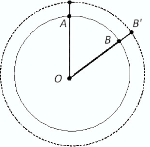
Figure 1: Brane model of Universe. Motion of particle from point A to point B(B’) in broadening Universe ( AB=$\nu\ d\tau,\ AB^{\prime}=c\ d\tau,\ BB^{\prime}=c\ dt$ ).

where $\nu^{2}=\left(dx^{1}/d\tau\right)^{2}$ + $\left(dx^{2}/d\tau\right)^{2}$ + $\left(dx^{3}/d\tau\right)^{2}$, $d\tau=dx^{0}/c.$ Geometrical meaning of relation(9) is explained in fig. 1.

Expression (6) can be rewritten in the following form:

$$p_{i}p^{j}=m^{2}c^{2}.$$ (10)

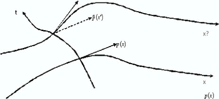
Figure 2: Coordinate transform at the excitation of membrane.

Let’s consider functional variation of relation (10) corresponding to brane fluctuation when coordinares x transform into coordinates x’ (fig. 2). Complete variation of momentum vector can be written as the sum of functional variation $\delta p$ of vector p at the comparison of p’ with p in the same point at the parallel transfer of vector p in universal space and ordinary variation dp. Then, it can be written that

$$\triangle p=p^{\prime}\left(x^{\prime}\right)-p\left(x\right)=p^{\prime}\left(x^{\prime}\right)-\stackrel{{\scriptstyle\sim}}{{p}}\left(x^{\prime}\right)+\stackrel{{\scriptstyle\sim}}{{p}}\left(x^{\prime}\right)-p\left(x\right)=\delta p+dp,$$ (11)

where

$$\delta p=p^{\prime}\left(x^{\prime}\right)-\ \stackrel{{\scriptstyle\sim}}{{p}}\left(x^{\prime}\right)$$ (12)

and

$$dp=\ \stackrel{{\scriptstyle\sim}}{{p}}\left(x^{\prime}\right)-p\left(x\right),$$ (13)

$\stackrel{{\scriptstyle\sim}}{{p}}\left(x^{\prime}\right)\$is momentum vector at its parallel transfer in the universal space.

If trajectory of particle is geodetic one then

$$dp_{i}=\frac{\partial p_{i}}{\partial x^{k}}dx^{k}=0,$$ (14)

$$\delta p_{i}=\stackrel{{\scriptstyle\sim}}{{p}}_{k}\Gamma_{il}^{k}\delta x^{l},$$ (15)

where $\delta x^{l}=x^{\prime l}-x^{l}$ is variation in universal space. Then, it can be written, omitting stroked index of momentum vector,

$$p\left(x^{\prime}\right)=p\left(x\right)+\delta p.$$ (16)

At the transform x $\rightarrow$ x’, relation (10) is transforming accounting (14) to the following form:

$$p_{i}p^{i}+p_{i}\delta p^{i}+\delta p_{i}p^{i}+\delta p_{i}\delta p^{i}=m^{2}c^{2}.$$ (17)

Let’s pass in relation (15) to operators acting in Hilbert space of wave functions $\psi\left(x\right)$. We represent for this sake the components of vector p as

$$p_{i}=-i\hbar\frac{\partial}{\partial x^{i}},$$ (18)

and rewrite relation (13) as

$$\delta p_{i}=-\left\{\Gamma_{i\alpha}^{k}\delta x^{\alpha}\right\}_{;k},$$ (19)

where covariant derivative is performed in the point with stroked indexes.

Let’s consider the first term in the left side of equation (15). For this purpose, we represent it in the form

$$p_{i}p^{i}=p_{i}g^{ij}p_{j}.$$ (20)

Using expression (16), we get

$$p_{i}p^{i}=-\hbar^{2}\left(\frac{\partial g^{ij}}{\partial x^{i}}\frac{\partial}{\partial x^{j}}+g^{ij}\frac{\partial^{2}}{\partial x^{i}\partial x^{j}}\right).$$ (21)

Let’s use well known relation

$$\frac{\partial g^{ij}}{\partial x^{k}}=-\Gamma_{mk}^{i}g^{mj}-\Gamma_{mk}^{j}g^{im}.$$ (22)

Then

$$p_{i}p^{i}=-\hbar^{2}\left(g^{ij}\frac{\partial^{2}}{\partial x^{i}\partial x^{j}}-g^{mj}\Gamma_{mk}^{i}\frac{\partial}{\partial x^{j}}-g^{im}\Gamma_{mk}^{j}\frac{\partial}{\partial x^{i}}\right).$$ (23)

Changing indexes of summation, we get

$$p_{i}p^{i}=-\hbar^{2}g^{ij}\left(\frac{\partial^{2}}{\partial x^{i}\partial x^{j}}-\Gamma_{ik}^{k}\frac{\partial}{\partial x^{j}}-\Gamma_{ij}^{k}\frac{\partial}{\partial x^{k}}\right).$$ (24)

Let’s consider second term in the left side of equation (15), rewriting it in the form

$$p_{i}\delta p^{i}=p_{i}g^{ij}\delta p_{j}.$$ (25)

Using formula (16), we get

$$p_{i}\delta p^{i}=g^{ij}p_{i}\delta p_{j}+i\hbar\left(g^{ij}\Gamma_{im}^{m}+g^{im}\Gamma_{im}^{j}\right)\delta p_{j}.$$ (26)

Let’s write in its direct form the covariant derivative in the expression (16):

$$\delta p_{j}=-i\hbar\left(\Gamma_{jk}^{i}+\frac{\partial\Gamma_{jl}^{k}}{\partial x^{k}}\delta x^{l}-\Gamma_{jk}^{n}\Gamma_{nl}^{k}\delta x^{l}+\Gamma_{nk}^{k}\Gamma_{jl}^{n}\delta x^{l}\right),$$ (27)

where stroked index of the derivative on is omitted. Substituting expression (27) into formula (26), we get

(35)

Third term in the left side of equation (15)

$$\delta p_{i}p^{i}=\delta p_{i}g^{ij}p_{j},$$ (36)

has according to expressions (16), (27) the following form:

$$\delta p_{i}p^{i}=-\hbar^{2}g^{ij}\left(\Gamma_{ik}^{k}+\frac{\partial\Gamma_{ij}^{k}}{\partial x^{k}}\delta x^{l}-\Gamma_{ik}^{n}\Gamma_{nl}^{k}\delta x^{l}+\Gamma_{nk}^{k}\Gamma_{il}^{n}\delta x^{l}\right)\frac{\partial}{\partial x^{j}}.$$ (37)

The last term in the left side of equation (15)

$$\delta p_{i}\delta p^{i}=\delta p_{i}g^{ij}\delta p_{j},$$ (38)

can be written with the account of expression (27) in the form

(50)

Substituting expressions (24), (35), (36) and (50) into equation (15), we get equation for the wave function $\psi$

(64)

Let’s consider covariant derivative of the second order for the wave function

$$\left\{\left\{\psi^{n}\right\}_{;i}\right\}_{;j}=\left\{\frac{\partial\psi^{n}}{\partial x^{i}}+\Gamma_{ik}^{n}\left(x^{\prime}\right)\psi^{k}\left(x^{\prime}\right)\right\}_{;j}=\frac{\partial^{2}\psi^{n}}{\partial x^{i}\partial x^{j}}-\Gamma_{ij}^{k}\frac{\partial\psi^{n}}{\partial x^{k}}-\Gamma_{ij}^{m}\Gamma_{mk}^{n}\psi^{k}\left(x^{\prime}\right).$$ (65)

If transformed wave function is still self function of energy operator, i.e. if with account of norm the relation

$$\psi^{n}\left(x\right)=\left(\Gamma_{ik}^{k}\right)^{-1}\Gamma_{ik}^{n}\psi^{k}\left(x^{\prime}\right),$$ (66)

is true, the first term in the equation (64) can be written in the form of covariant D’Alambertian

$$g^{ij}\left(\frac{\partial^{2}}{\partial x^{i}\partial x^{j}}-\Gamma_{ij}^{k}\frac{\partial}{\partial x^{k}}-\Gamma_{ij}^{m}\Gamma_{mk}^{n}\right)\psi=g^{ij}D_{i}D_{j}\psi.$$ (67)

It is evident that the expression in brackets in the second term in the left side of equation (64) is just Richey’s tensor and we can write

$$g^{ij}\left(\frac{\partial\Gamma_{jk}^{k}}{\partial x^{i}}-\frac{\partial\Gamma_{ij}^{k}}{\partial x^{k}}+\Gamma_{in}^{k}\Gamma_{jk}^{n}-\Gamma_{ij}^{n}\Gamma_{nk}^{k}\right)\psi=-g^{ij}R_{ij}\psi.$$ (68)

We assume that $\delta x^{l}=0\$for coordinates on brane and $\delta x^{l}\neq 0\$for coordinates along the additional dimension. Then, assuming that coefficients of affine connection on brane do not depend on the coordinate of additional dimension, it could be written

$$g^{ij}\left(\Gamma_{jk}^{n}\frac{\partial\Gamma_{nl}^{k}}{\partial x^{i}}+\Gamma_{nl}^{k}\frac{\partial\Gamma_{jk}^{n}}{\partial x^{i}}-\Gamma_{nk}^{k}\frac{\partial\Gamma_{jl}^{n}}{\partial x^{i}}-\Gamma_{jl}^{n}\frac{\partial\Gamma_{nk}^{k}}{\partial x^{i}}-\frac{\partial^{2}\Gamma_{jl}^{k}}{\partial x^{i}\partial x^{k}}\right)=-g^{ij}\frac{\partial R_{jl}}{\partial x^{i}},$$ (69)

$$g^{ij}\left(\Gamma_{ij}^{m}\frac{\partial\Gamma_{lm}^{k}}{\partial x^{k}}-\Gamma_{ij}^{m}\Gamma_{mk}^{n}\Gamma_{l\ n}^{k}+\Gamma_{ij}^{m}\Gamma_{nk}^{k}\Gamma_{lm}^{n}\right)=g^{ij}\Gamma_{ij}^{m}R_{ml},$$ (70)

$$g^{ij}\left(\Gamma_{im}^{m}\frac{\partial\Gamma_{jl}^{k}}{\partial x^{k}}-\Gamma_{im}^{m}\Gamma_{jk}^{n}\Gamma_{nl}^{k}+\Gamma_{im}^{m}\Gamma_{nk}^{k}\Gamma_{jl}^{n}\right)=g^{ij}\Gamma_{im}^{m}R_{jl},$$ (71)

$$g^{ij}\left(\frac{\partial\Gamma_{il}^{k}}{\partial x^{k}}-\Gamma_{ik}^{n}\Gamma_{nl}^{k}+\Gamma_{nk}^{k}\Gamma_{il}^{n}\right)=g^{ij}R_{il}.$$ (72)

Relations (69),(70) yield

$$g^{ij}\frac{\partial R_{jl}}{\partial x^{i}}-g^{ij}\Gamma_{ij}^{m}R_{ml}=g^{ij}D_{i}R_{jl}.$$ (73)

Using the same approach that at the derivation of relation (67), we get from formulas (71),(72)

$$g^{ij}R_{il}\frac{\partial\psi_{n}}{\partial x^{i}}-g^{ij}\Gamma_{im}^{m}R_{il}\psi_{n}=g^{ij}R_{jl}D_{i}\psi_{n}.$$ (74)

Unifying expressions (73),(74), we get

$$g^{ij}\left(D_{i}R_{il}\right)\psi_{n}-g^{ij}R_{il}D_{i}\psi_{n}=g^{ij}D_{i}\left(R_{jl}\psi\right).$$ (75)

Last term in the left side of equation (64) can be written as

$$g^{ij}\left(\frac{\partial\Gamma_{il}^{k}}{\partial x^{k}}-\Gamma_{ik}^{m}\Gamma_{ml}^{k}+\Gamma_{mk}^{k}\Gamma_{il}^{m}\right)\left(\frac{\partial\Gamma_{jl^{\prime}}^{n}}{\partial x^{n}}-\Gamma_{jn}^{m^{\prime}}\Gamma_{m^{\prime}l^{\prime}}^{n}+\Gamma_{m^{\prime}n}^{n}\Gamma_{jl^{\prime}}^{m^{\prime}}\right)\delta x^{l}\delta x^{l^{\prime}}\psi=g^{ij}R_{il}R_{il^{\prime}}\delta x^{l}\delta x^{l^{\prime}}\psi.$$ (76)

Thus, equation (64) can be rewritten in the following form:

$$g^{ij}D_{i}D_{j}\psi_{n}-g^{ij}R_{il}D_{i}\psi_{n}+g^{ij}D_{i}\left(R_{jl}\psi_{n}\right)\delta x^{l}+g^{ij}R_{il}R_{il^{\prime}}\delta x^{l}\delta x^{l^{\prime}}\psi_{n}+m^{2}c^{2}=0..$$ (77)

Let’s consider small region of space-time where we can suppose gravitation field to be constant and homogeneous. We rewrite equation (77) in locally-geodesic coordinate system for mass-less particle in the following form:

$$\left\{\frac{\partial^{2}}{\partial x^{2}}+\gamma\frac{\partial}{\partial x}+\alpha\right\}\psi=\frac{1}{c^{2}}\frac{\partial^{2}\psi}{\partial t^{2}},$$ (78)

limiting ourselves by one spatial dimension, assuming the absence of affine connection in time and introducing the notations

$$\gamma=R_{x\theta}\delta x^{\theta}$$ (79)

and

$$\alpha=R-\left(\frac{\partial}{\partial x}R_{x\theta}\right)\delta x^{\theta}-R_{x\theta}R_{x\theta^{\prime}}\delta x^{\theta}\delta x^{\theta^{\prime}}.$$ (80)

Let’s look for solution in the form

$$\psi=e^{i\left(kx-\omega t\right)}.$$ (81)

Then we get from (78) the characteristic equation

$$k^{2}-i\gamma k-\left(\alpha+\frac{\omega^{2}}{c^{2}}\right)=0.$$ (82)

Its physically reasonable solution is

$$k=\sqrt{\frac{\omega^{2}}{c^{2}}+\alpha-\frac{\gamma^{2}}{4}}+i\frac{\gamma}{2}.$$ (83)

Apparently it is valid when a does not depend on coordinate and time. When $\alpha=\gamma=0,$ we have the usual dispersion relation $\omega_{0}=ck.$

When $\left(\frac{\omega}{c}\right)\gg\alpha-\left(\frac{\gamma}{2}\right)^{2}$we can approximately get

$$k=\frac{\omega}{c}\left(1+\frac{c^{2}}{\omega^{2}}\left(\alpha-\frac{\gamma^{2}}{4}\right)\right)+i\frac{\gamma}{2}$$ (84)

and for phase velocity of non-massive particles

$$\frac{dk}{d\omega}=c\left(1+\frac{c^{2}}{\omega^{2}}\left(\alpha-\frac{\gamma^{2}}{4}\right)\right).$$ (85)

Formula (85) shows that effective refractive index related with space curvature is equal

$$n_{eff}=1-\frac{c^{2}}{\omega^{2}}\left(\alpha-\frac{\gamma^{2}}{4}\right).$$ (86)

Thus, the phase velocity of mass-less particles in universal space can exceed the phase velocity of light in plane Deckard space because of drift of particles at the expansion of Universe. Other consequences of space curvature are the following two facts that realize when expression (86) is valid:

- it is impossible to create particle with kinetic energy less than $\hbar\sqrt{\omega^{2}+\alpha c^{2}}$ (fig. 3);

- space curvature leads to the frequency shift according the formula $\omega=\sqrt{\omega_{0}^{2}+\alpha c^{2}}$ that gives the possibility for verification of developed model when curvature varies at the influence of gravitational waves and primordial fluctuations.

Note that it could also represent the more complexity solution of equation (47) in the form:

$$\psi=e^{-\frac{1}{2}x\left(\gamma-\sqrt{\gamma^{2}-4\alpha}\right)}\left(\alpha+\beta\ e^{x\left(\gamma-\sqrt{\gamma^{2}-4\alpha}\right)}\right)+A\ e^{ct\sqrt{\alpha}}+B\ e^{-ct\sqrt{\alpha}}.$$ (87)

where A, B and $\beta$ are an arbitrary constants of integration.

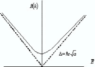
Figure 3: Energy of moving particle E(k)=ck.