Generic short-range interactions in two-leg ladders

Abstract

We derive a Hamiltonian for a two-leg ladder which includes an arbitrary number of charge and spin interactions. To illustrate this Hamiltonian we consider two examples and use a renormalization group technique to evaluate the ground state phases. The first example is a two-leg ladder with zigzagged legs. We find that increasing the number of interactions in such a two-leg ladder may result in a richer phase diagram, particularly at half-filling where a few exotic phases are possible when the number of interactions are large and the angle of the zigzag is small. In the second example we determine under which conditions a two-leg ladder at quarter-filling is able to support a Tomanaga-Luttinger liquid phase. We show that this is only possible when the spin interactions across the rungs are ferromagnetic. In both examples we focus on lithium purple bronze, a two-leg ladder with zigzagged legs which is though to support a Tomanaga-Luttinger liquid phase.

I Introduction

Ladder systems are well known for their many novel properties and their relative simplicity makes them an ideal candidate for much theoretical work. Dagotto96 ; Maekawa96 Several experimental systems are known to be of or dominated by a ladder-type structure, and theoretical studies have been able to make reasonable predictions about the phases, symmetries and transport properties of these materials. Scalapino95 ; Mayaffre98 ; Blumberg02 A common procedure used to solve ladder systems is a perturbative renormalization group (RG) treatment, followed by a non-perturbative bosonization of the relevant interactions. The combination of these two complimentary techniques allows one to go beyond the usual mean-field approaches when determining ground states and excitations in the low-energy regime. Lin98 Some studies using these techniques have revealed exotic phases, such as a staggered-flux phase Fjaerestad02 and a resonant-valence-bond liquid. Lin98

In a recent experiment, Wang06 it was demonstrated that Tomanaga-Luttinger liquid (TLL) behavior appears in lithium purple bronze Li_0.9Mo₆O₁₇ (LPB). It is rather remarkable that typical TLL scaling appears to exist over a wide range of temperatures. In this reference it was claimed that RG flows quantitatively reproduce the experimental data, but the bare interactions which lead to this solution were not discussed. This exciting development inspired us to revisit the well-known two-leg ladder system, modified to describe a realistic interaction profile while also taking into account the ladder geometry, as shown in Fig. 1.

A standard two-leg ladder is shown in Fig. 1(a). The hopping strengths between nearest neighbors on the same leg and nearest neighbors on the same rung are $t$ and $t_{\perp}$ respectively. For on-site interactions the charge and spin interactions take the same form and can be described by a single parameter $U$. In general, interactions between two different lattice sites along the same leg are described by $X_{\parallel n}$, while interactions between two lattice sites on opposite legs are described by $X_{\perp n}$. The charge and spin interactions are represented by $X=V,J$ respectively and the integer index $n$ describes the rung difference between the two sites. Therefore, any set of generic short-range or quasi-long-range interactions can be described by the bare interactions $U$, $X_{\parallel n}$ and $X_{\perp n}$. Although there have been extensive theoretical investigations on electronic correlations in two-leg ladders, Lin98 ; Fjaerestad02 ; Tsuchiizu02 ; Wu03 ; Tsuchiizu05 ; Chitov08 most of these studies only consider nearest-neighbor (or next-nearest-neighbor) interactions.

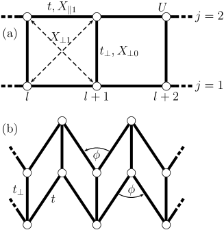
Figure 1: (a) A standard two-leg ladder with hopping strengths $t$ and $t_{\perp}$ and several electron-electron interactions defined by $U$ and $X$ where $X=V,J$. (b) A zigzag two-leg ladder where the legs are bent to make a constant angle $\phi$. Electron-electron interactions can be defined similarly to the standard case.

The standard two-leg ladder lies in a two-dimensional plane, but there are a number of experimental systems which contain a two-leg ladder which is warped in some fashion. Popovic06 ; Brunger08 We consider a ladder which has been compressed so that the legs form a zigzag with a constant angle $\phi$, as shown in Fig. 1(b). One example of such a lattice is LPB which has $\phi\sim\pi/2$. Popovic06 By including the geometric structure of the two-leg ladder we have an additional variable $\phi$ with which to investigate the ground-state phase diagram. It is easy to see that for extremely short-range interactions the zigzag angle $\phi$ does not play any significant role since the on-site interaction $U$ dominates. However, in ladder materials the interaction is often expected to be quasi-long-ranged and in these cases $\phi$ is important. With the inclusion of this zigzag lattice geometry, as well as the generic interactions we hope to not only be able to fully describe a TLL phase but to also discover other exotic phases such as an $f$-density wave and a staggered-flux phase.

The Tomanaga-Luttinger liquid is a special case amongst all the possible phases of a two-leg ladder. In sharp contrast to ordinary Fermi liquids, electron-electron interactions in TLL cause the single-particle excitations (the so-called quasi-particles) to become unstable. Instead one finds bosonic spin and charge excitations which propagate independently of each other and with different velocities, a phenomenon known as spin-charge separation. Many theoretical and experimental studies have discussed TLL phase in several different 1D or quasi-1D systems such as weakly-coupled chains or wires, Kim96 ; Segovia99 carbon nanotubes, Bockrath99 ; Ishii03 and the edges of two-dimensional systems. Wen90 ; Hilke01 With screened charge interactions theoretical studies have shown that TLL are generally expected in odd-leg ladders Ledermann00 but not in even-leg ladders except under unphysical conditions such as attractive interactions. Lin98 These general trends make the TLL scaling behavior observed in LPB Popovic06 ; Wang06 a little unexpected, though as the two legs in LPB are almost independent ($t\gg t_{\perp}$) it is certainly not impossible. There are two plausible scenarios for the observed TLL-like behavior in LPB. The first scenario is that the ground state is a true TLL and that the interaction profile and the ladder geometry in LPB result in an unusual set of bare couplings that flow towards the TLL phase under RG transformations. The alternative possibility is that the ground state is not a TLL but closely resembles a TLL over a wide range of temperatures. In an attempt to solve this puzzle we will use LPB as an example when determining the phases of our two-leg ladder with zigzagged legs and generic interactions.

This paper is organized in the following way: In Sec. II, we introduce the two-leg model that contains various charge and spin interactions. Starting from the lattice model, we briefly describe the chiral decomposition, current algebra, computation of initial couplings and the bosonization. In Sec. III, we generalize the theoretical approach to the two-leg ladder with general zigzag angles. We also introduce different order parameters to characterize the ground states. The complimentary combination of the RG method and the bosonization techniques allows us to obtain the phase diagrams for different interaction profiles and bending angles. We consider two examples, the half-filled case with $t=t_{\perp}$ and the quarter-filled case with $t\gg t_{\perp}$, with the latter case corresponding to LPB. In Sec. IV, we make use of the general theoretical framework developed in previous sections and try to determine an appropriate interaction profile for a TLL in LPB. We perform detailed and extensive numerical analysis and compute the temperature-dependent TLL exponent. Finally, we conclude our numerical results and discuss their connections to experiments.

II Model

We consider a two-leg ladder with quasi-long-range charge and spin interactions. The Hamiltonian contains non-interacting hopping as well as charge and spin interactions over different ranges. Thus, it is natural to divide the Hamiltonian into six parts,

$$H=H_{0}+H_{U}+H_{V_{\perp}}+H_{V_{\parallel}}+H_{J_{\perp}}+H_{J_{\parallel}}.$$ (1)

The first term $H_{0}$ describes hopping along the legs of the ladder with hopping strength $t$, and along the rungs with hopping strength $t_{\perp}$,

$$H_{0}= -t\sum_{jl\sigma}(c_{jl\sigma}^{{\dagger}}c_{j(l+1)\sigma}+h.c.)$$

$$-t_{\perp}\sum_{l\sigma}(c_{1l\sigma}^{{\dagger}}c_{2l\sigma}+h.c.).$$ (2)

The subscript of the fermion operator $c_{jl\sigma}$ describes leg number $j=1,2$, rung number $l$, and spin $\sigma=\uparrow,\downarrow$.

For the on-site interaction, the difference between the charge and the spin parts vanishes and

$$H_{U}=U\sum_{jl}n_{jl\uparrow}n_{jl\downarrow}$$ (3)

where $n_{jl\sigma}=c_{jl\sigma}^{{\dagger}}c_{jl\sigma}$ and $U$ is the interaction strength. Now we classify the more general charge interactions. Many theoretical studies consider perpendicular nearest neighbor interactions across single rungs, i.e., between sites $(j,l)$ and $(\bar{\jmath},l)$ where $\bar{\jmath}$ denotes the opposite leg of $j$, as well as parallel nearest neighbor interactions between neighboring sites on the same leg, i.e., between sites $(j,l)$ and $(j,l\pm 1)$. A few studies also consider next-nearest neighbor interactions which act diagonally across one plaquette, i.e, between sites $(j,l)$ and $(\bar{\jmath},l\pm 1)$. Here we consider all charge interactions between sites $(j,l)$ and $(j^{\prime},l^{\prime})$ for which $|l-l^{\prime}|\leq N$. Note that we have introduced a “hard” cutoff length $N$ for the interaction profile. The perpendicular Hamiltonian describes interactions between sites on different legs

$$H_{V_{\perp}}=\sum_{n=0}^{N}\sum_{jl\sigma\sigma^{\prime}}V_{\perp n}n_{jl\sigma}n_{\bar{\jmath}(l+n)\sigma^{\prime}}$$ (4)

where $V_{\perp n}$ is the interaction strength between sites $(j,l)$ and $(\bar{\jmath},l+n)$. The parallel Hamiltonian describes interactions between sites on the same leg

$$H_{V_{\parallel}}=\sum_{n=1}^{N}\sum_{jl\sigma\sigma^{\prime}}V_{\parallel n}n_{jl\sigma}n_{j(l+n)\sigma^{\prime}}$$ (5)

where $V_{\parallel n}$ is the interaction strength between sites $(j,l)$ and $(j,l+n)$.

Following the same classification the spin interactions are contained in two parts, $H_{J_{\perp}}$ and $H_{J_{\parallel}}$. Like $H_{V_{\perp}}$ and $H_{V_{\parallel}}$, the spin interaction Hamiltonians describe interactions between any two sites which are $N$ or less rung positions distant from each other. For spin interactions between sites on different rungs,

$$H_{J_{\perp}}=\sum_{n=0}^{N}\sum_{jl}J_{\perp n}{\bf S}_{jl}\cdot{\bf S}_{\bar{\jmath}(l+n)}$$ (6)

where $J_{\perp n}$ is the interaction strength between sites $(j,l)$ and $(\bar{\jmath},l+n)$ and the spin operators are

$${\bf S}_{jl}={\textstyle{\frac{1}{2}}}\sum_{\sigma\sigma^{\prime}}c^{{\dagger}}_{jl\sigma}\bm{\tau}_{\sigma\sigma^{\prime}}c_{jl\sigma^{\prime}},$$ (7)

where $\boldsymbol{\tau}=(\tau_{x},\tau_{y},\tau_{z})$ are Pauli matrices. For spin interaction between different sites on the same leg,

$$H_{J_{\parallel}}=\sum_{n=1}^{N}\sum_{jl\sigma\sigma^{\prime}}J_{\parallel n}{\bf S}_{jl}\cdot{\bf S}_{j(l+n)}$$ (8)

where $J_{\parallel n}$ is the interaction strength between sites $(j,l)$ and $(j,l+n)$.

We now follow a standard procedure which involves decomposing the lattice fermions into pairs of chiral fermions with linear dispersion. As this procedure is well explained elsewhere Lin98 we will only give a brief explanation. Firstly, the hopping part of the Hamiltonian $H_{0}$ is diagonalized into a bonding and antibonding band, $a_{ql\sigma}=[c_{2l\sigma}-(-1)^{q}c_{1l\sigma}]/\sqrt{2}$ with $q=1,2$, then after a Fourier transform we can determine the band structure $E_{q}=(-1)^{q}t_{\perp}-2t\cos k_{q}$ as a function of momentum $k_{q}$. The Fermi momentum $k_{Fq}=\cos^{-1}[(-\mu+(-1)^{q}t_{\perp})/2t]$ is uniquely determined by the chemical potential $\mu$. As we are only interested in the low-energy behavior the fermion operators which diagonalize the hopping Hamiltonian can be linearized about the Fermi point by introducing chiral fermion fields, $a_{ql\sigma}\sim\psi_{Rql\sigma}e^{ik_{Fq}l}+\psi_{Lql\sigma}e^{-ik_{Fq}l}$. Taking the continuous limit of the discrete lattice index $l$, we can define the Hamiltonian density $\mathcal{H}$ from $H=\int dl\mathcal{H}$. The hopping part of the Hamiltonian density in terms of the chiral fields is rather simple,

$$\mathcal{H}_{0}=-\sum_{q\sigma}v_{q}(\psi^{{\dagger}}_{Rql\sigma}\partial_{l}\psi_{Rql\sigma}-\psi^{{\dagger}}_{Lql\sigma}\partial_{l}\psi_{Lql\sigma})$$ (9)

where the Fermi velocity is $v_{q}=dE_{q}/dk_{q}$ at $k_{q}=k_{Fq}$.

The interaction part of the Hamiltonian density $\mathcal{H}_{I}=\mathcal{H}_{U}+\mathcal{H}_{V_{\perp}}+\mathcal{H}_{V_{\parallel}}+\mathcal{H}_{J_{\perp}}+\mathcal{H}_{J_{\parallel}}$ can be expressed in terms of the currents

$$J_{Pqq^{\prime}}= {\textstyle{\frac{1}{2}}}\psi^{{\dagger}}_{Pq\sigma}\psi_{Pq^{\prime}\sigma},\,\, {\mathbf{J}}_{Pqq^{\prime}} ={\textstyle{\frac{1}{2}}}\psi^{{\dagger}}_{Pq\sigma}\boldsymbol{\tau}_{\sigma\sigma^{\prime}}\psi_{Pq^{\prime}\sigma^{\prime}}$$

$$I_{Pqq^{\prime}}= {\textstyle{\frac{1}{2}}}\psi_{Pq\sigma}\epsilon_{\sigma\sigma^{\prime}}\psi_{Pq^{\prime}\sigma^{\prime}},\,\, {\mathbf{I}}_{Pqq^{\prime}} ={\textstyle{\frac{1}{2}}}\psi_{Pq\sigma}(\epsilon\boldsymbol{\tau})_{\sigma\sigma^{\prime}}\psi_{Pq^{\prime}\sigma^{\prime}}$$ (10)

where $P=R,L$. The antisymmetric matrix $\epsilon$ is defined by $\epsilon_{12}=-\epsilon_{21}=1$ and $\epsilon_{11}=\epsilon_{22}=0$. Each term in $\mathcal{H}_{I}$ is a product of two currents so that the Hamiltonian is a function of four-fermion interactions,

$$\mathcal{H}_{I}= b^{\rho}_{qq^{\prime}}J_{Rqq^{\prime}}J_{Lqq^{\prime}}-b^{\sigma}_{qq^{\prime}}{\mathbf{J}}_{Rqq^{\prime}}.{\mathbf{J}}_{Lqq^{\prime}}$$

$$+f^{\rho}_{qq^{\prime}}J_{Rqq}J_{Lq^{\prime}q^{\prime}}-f^{\sigma}_{qq^{\prime}}{\mathbf{J}}_{Rqq}.{\mathbf{J}}_{Lq^{\prime}q^{\prime}}$$

$$+u^{\rho}_{qq^{\prime}}I^{{\dagger}}_{qq^{\prime}}I_{L\bar{q}\bar{q}^{\prime}}-u^{\sigma}_{qq^{\prime}}{\mathbf{I}}_{Rqq^{\prime}}.{\mathbf{I}}_{L\bar{q}\bar{q}^{\prime}}.$$ (11)

The couplings of the four-fermion interactions $b_{qq^{\prime}}$, $f_{qq^{\prime}}$ and $u_{qq^{\prime}}$ define the scattering amplitudes between bands $q$ and $q^{\prime}$. Backward scattering is represented by $b$ and from a gradient expansion the bare coupling strength can be shown to be

$$b^{\rho}_{qq}= U+V_{\perp 0}+2\sum_{n=1}^{N}[(V_{\parallel n}+V_{\perp n})(2-\cos 2nk_{Fq})]$$

$$-{\textstyle{\frac{3}{4}}}J_{\perp 0}-{\textstyle{\frac{3}{2}}}\sum_{n=1}^{N}[(J_{\parallel n}+J_{\perp n})\cos 2nk_{Fq}]$$

$$b^{\sigma}_{qq}= U+V_{\perp 0}+2\sum_{n=1}^{N}[(V_{\parallel n}+V_{\perp n})\cos 2nk_{Fq}]$$

$$-{\textstyle{\frac{3}{4}}}J_{\perp 0}-\sum_{n=1}^{N}[(J_{\parallel n}+J_{\perp n})(1+{\textstyle{\frac{1}{2}}}\cos 2nk_{Fq})]$$

$$b^{\rho}_{12}= U-V_{\perp 0}+2\sum_{n=1}^{N}[(V_{\parallel n}-V_{\perp n})(2\cos nk_{-}-\cos nk_{+})]$$

$$+{\textstyle{\frac{3}{4}}}J_{\perp 0}-{\textstyle{\frac{3}{2}}}\sum_{n=1}^{N}[(J_{\parallel n}-J_{\perp n})\cos nk_{+}]$$

$$b^{\sigma}_{12}= U-V_{\perp 0}+2\sum_{n=1}^{N}[(V_{\parallel n}-V_{\perp n})\cos nk_{+}]$$

$$+{\textstyle{\frac{3}{4}}}J_{\perp 0}-\sum_{n=1}^{N}[(J_{\parallel n}-J_{\perp n})(\cos nk_{-}+{\textstyle{\frac{1}{2}}}\cos nk_{+})]$$ (12)

where $k_{\pm}=k_{F1}\pm k_{F2}$. The symmetry of the system requires $b_{12}=b_{21}$ and at half-filling $\mu=0$ so $k_{F1}+k_{F2}=\pi$ which sets $b_{11}=b_{22}$. Forward scattering is represented by $f$ with the bare coupling strength,

$$f^{\rho}_{12}= U+2\sum_{n=1}^{N}[V_{\parallel n}(2-\cos nk_{+})+V_{\perp n}(2+\cos nk_{+})]$$

$$+3V_{\perp 0}+{\textstyle{\frac{3}{4}}}J_{\perp 0}-{\textstyle{\frac{3}{2}}}\sum_{n=1}^{N}[(J_{\parallel n}-J_{\perp n})\cos nk_{+}]$$

$$f^{\sigma}_{12}= U-V_{\perp 0}+2\sum_{n=1}^{N}[(V_{\parallel n}-V_{\perp n})\cos nk_{+}]-{\textstyle{\frac{1}{4}}}J_{\perp 0}$$

$$-\sum_{n=1}^{N}[J_{\parallel n}(1+{\textstyle{\frac{1}{2}}}\cos nk_{+})-J_{\perp n}(1-{\textstyle{\frac{1}{2}}}\cos nk_{+})].$$ (13)

Symmetry requires $f_{12}=f_{21}$ and in order to avoid double counting we set $f_{qq}=0$. Umklapp scattering is represented by $u$ and only present at half-filling where $k_{F1}+k_{F2}=\pi$,

$$u^{\rho}_{11}= U-V_{\perp 0}+2\sum_{n=1}^{N}[(V_{\parallel n}-V_{\perp n})(-1)^{n}]$$

$$+{\textstyle{\frac{3}{4}}}J_{\perp 0}-{\textstyle{\frac{3}{2}}}\sum_{n=1}^{N}[(J_{\parallel n}-J_{\perp n})(-1)^{n}]$$

$$u^{\rho}_{12}= 2U+2\sum_{n=1}^{N}[V_{\parallel n}(\cos 2nk_{F1}+(-1)^{n})$$

$$+V_{\perp n}(\cos 2nk_{F1}-(-1)^{n})]$$

$$-{\textstyle{\frac{3}{2}}}\sum_{n=1}^{N}[J_{\parallel n}(\cos 2nk_{F1}+(-1)^{n})$$

$$-J_{\perp n}(\cos 2nk_{F1}-(-1)^{n})]$$

$$u^{\sigma}_{12}= 2V_{\perp 0}+2\sum_{n=1}^{N}[V_{\parallel n}(\cos 2nk_{F1}-(-1)^{n})$$

$$+V_{\perp n}(\cos 2nk_{F1}+(-1)^{n})+{\textstyle{\frac{1}{2}}}J_{\perp 0}$$

$$+{\textstyle{\frac{1}{2}}}\sum_{n=1}^{N}[J_{\parallel n}(\cos 2nk_{F1}-(-1)^{n})$$

$$+J_{\perp n}(\cos 2nk_{F1}+(-1)^{n})]$$ (14)

with $u_{12}=u_{21}$ and $u_{11}=u_{22}$ from symmetry. At half-filling, the particle-hole symmetry ensures we have nine unique coupling constants, $b^{\rho}_{11}=b^{\rho}_{22}$, $b^{\sigma}_{11}=b^{\sigma}_{22}$, $b^{\rho}_{12}$, $b^{\sigma}_{12}$, $f^{\rho}_{12}$, $f^{\sigma}_{12}$, $u^{\rho}_{11}=u^{\rho}_{22}$, $u^{\rho}_{12}$ and $u^{\sigma}_{12}$. Away from half-filling the Umklapp interactions vanish but we no longer have $b_{11}=b_{22}$ so we have eight different coupling constants.

The Hamiltonian is more easily analyzed if the chiral fermion operators are replaced with boson operators. Lin98 ; vonDelft98 The bosonized fields $\theta_{\nu\pm}$ and $\varphi_{\nu\pm}$ with $\nu=\rho,\sigma$ represent a variety of quantum numbers. The subscript represents total (+) or relative (-) charges or spins ($\rho$ or $\sigma$ respectively) between the two bands while $\theta$ is a displacement field and $\varphi$ is a phase field. The total bosonized Hamiltonian density $\mathcal{H}=\mathcal{H}_{0}+\mathcal{H}_{I}$ is

$$\mathcal{H}=\frac{1}{8\pi}\sum_{\nu\pm}v_{\nu\pm}[K_{\nu\pm}^{-1}(\partial_{x}\theta_{\nu\pm})^{2}+K_{\nu\pm}(\partial_{x}\varphi_{\nu\pm})^{2}]\\ -2b^{\sigma}_{12}\cos\varphi_{\rho-}\cos\theta_{\sigma+}+2\cos\theta_{\sigma+}(b^{\sigma}_{11}\cos\theta_{\sigma-}\\ +f^{\sigma}_{12}\cos\varphi_{\sigma-})-\cos\varphi_{\rho-}(b^{+}_{12}\cos\theta_{\sigma-}+b^{-}_{12}\cos\varphi_{\sigma-})\\ -2u^{\rho}_{11}\cos\theta_{\rho+}\cos\varphi_{\rho-}-2u^{\sigma}_{12}\cos\theta_{\rho+}\cos\theta_{\sigma+}\\ -\cos\theta_{\rho+}(u^{+}_{12}\cos\theta_{\sigma-}+u^{-}_{12}\cos\varphi_{\sigma-})$$ (15)

where $b^{\pm}_{12}=b^{\sigma}_{12}\pm b^{\rho}_{12}$ and $u^{\pm}_{12}=u^{\sigma}_{12}\pm u^{\rho}_{12}$. The Luttinger parameters and the Fermi velocities for the total/relative charge and spin sectors are

$$K_{\nu\pm}= \sqrt{\frac{2\pi(v_{1}+v_{2})-[(b^{\nu}_{11}+b^{\nu}_{22})/2\pm f^{\nu}_{12}]}{2\pi(v_{1}+v_{2})+[(b^{\nu}_{11}+b^{\nu}_{22})/2\pm f^{\nu}_{12}]}}$$ (16)

$$v_{\nu\pm}= \sqrt{4\pi^{2}(v_{1}+v_{2})^{2}-[(b^{\nu}_{11}+b^{\nu}_{22})/2\pm f^{\nu}_{12}]^{2}}/4\pi.$$

Note that the highly symmetric bosonized form in Eq. (15) is possible only for degenerate velocity $v_{1}=v_{2}$. This is always true at half-filling but not at generic fillings. The LPB two-leg ladder we are interested in is at quarter-filling, Popovic06 but as it consists of nearly independent chains with vanishingly small inter-chain hopping $t_{\perp}\ll t$, the Fermi velocities are nearly degenerate $v_{1}\sim v_{2}$ and the above bosonized Hamiltonian is valid.

The RG flow equations of the couplings are of the form $dg_{i}/d\ell=\sum_{jk}A^{jk}_{i}g_{j}g_{k}$, where $A^{jk}_{i}$ is a constant tensor that can be computed from operator product expansions. Lin98 ; Chang05 All RG flow equations are solved simultaneously with the initial conditions at $\ell=0$ given in Eqs. (12-14). The ground state phase is determined from a non-zero order parameter, such as electron density or current flow, which can be evaluated using the solutions of the RG flow equations. On substituting the RG solutions into the bosonized Hamiltonian Eq. (15) the Hamiltonian may be minimized by a specific set of pinned bosonized fields (while other fields remain free to adopt any value), thus defining the ground state. For example, if $b^{\sigma}_{12}$ flows to a non-zero value then $b^{\sigma}_{12}\cos\varphi_{\rho-}\cos\theta_{\sigma+}$ in Eq. (15) could minimize the Hamiltonian by pinning $\varphi_{\rho-},\theta_{\sigma+}=m\pi$ for some integer $m$. In order to maintain this minimum, $m$ can change by integral values, which describes an excitation over some finite energy gap. If instead $b^{\sigma}_{12}$ flows to zero the term $b^{\sigma}_{12}\cos\varphi_{\rho-}\cos\theta_{\sigma+}$ is irrelevant. Any field that remains unpinned when the Hamiltonian is minimized may describe a gapless excitation. The pinned fields may be substituted into the order parameter equations, once they are appropriately bosonized, to determine the phase. Therefore, each phase can essentially be defined by a unique set of pinned boson fields, which are directly related to the solutions of the RG flow equations. Note that it is only the coefficients of the sinusoidal terms which ultimately determine the gapped excitations and therefore $b^{\rho}_{qq}$ and $f^{\rho}_{12}$ are the only couplings which can be non-zero in a fully gapless phase, i.e., a TLL.

III Zigzag two-leg ladder

Now we would like to incorporate the realistic ladder geometry into the above theoretical model. We consider a two-leg ladder in which the legs zigzag parallel to each other, as shown in Fig. 1(b). The bent legs make a constant angle $\phi$. For unscreened charge interactions the interaction strengths between two sites are inversely proportional to the distance between them so,

$$X_{\parallel n}= \frac{X}{an\sin\phi/2},\qquad n=2,4,6,...$$

$$X_{\parallel n}= \frac{X}{a\sqrt{1+(n^{2}-1)\sin\phi/2}},\qquad n=1,3,5,...$$

$$X_{\perp n}= \frac{X}{a\sqrt{\delta^{2}+n^{2}\sin^{2}\phi/2}},\qquad n=0,2,4,...$$

$$X_{\perp n}= \frac{X}{a\sqrt{1+\delta^{2}+(n^{2}-1)\sin\phi/2}},\qquad n=1,3,5,...$$ (17)

where $X=V,J$, $a$ is the distance between neighboring lattice sites on the same leg and the distance between lattice sites on the same rung is $a\delta$. We shall assume the ladder consists of square plaquettes with $\delta=1$. Generally we would like interactions beyond the cutoff, i.e., with $n>N$, to be less strong than interactions within the cutoff, but when $\phi$ is very small this may not be the case. This issue may be avoided by defining different cutoffs for interactions along a leg and interactions between legs, but as the small values of $\phi$ for which this problem occurs are quite likely not experimentally attainable we will continue to use just one cutoff $N$.

III.1 Order parameters

At half-filling the phase of a two-leg ladder could be one of four density wave phases or one of four Mott insulator phases. Tsuchiizu02 ; Tsuchiizu05 We first discuss the density wave phases, the charge density wave (CDW), the staggered-flux (SF) phase, the $p$-density wave (PDW) and the $f$-density wave (FDW), and their associated order parameters. A CDW has a non-zero variation in the average electron density per site which is defined by

$$n_{jl}=\sum_{\sigma}c^{{\dagger}}_{jl\sigma}c_{jl\sigma}.$$ (18)

At half-filling the average electron density of a two-leg ladder is one electron per site, but in a CDW the sites are alternatively unoccupied or fully occupied by two electrons. To define current flow we use

$$j_{\perp jl}= i\sum_{\sigma}[c^{{\dagger}}_{\bar{\jmath}l\sigma}c_{jl\sigma}-h.c.]$$

$$j_{\parallel jl}= i\sum_{\sigma}[c^{{\dagger}}_{j(l+1)\sigma}c_{jl\sigma}-h.c.]$$

$$j_{djl}= i\sum_{\sigma}[c^{{\dagger}}_{\bar{\jmath}(l+1)\sigma}c_{jl\sigma}-h.c.]$$ (19)

which describe currents along rungs between sites $(j,l)$ and $(\bar{\jmath},l)$, along legs between sites $(j,l)$ and $(j,l+1)$ and along the diagonals of the plaquettes between sites $(j,l)$ and $(\bar{\jmath},l+1)$, respectively. If the first two currents are non-zero we have a SF phase which is characterized by alternative clockwise and anticlockwise current flows around plaquettes. If the third current is non-zero we have a FDW which is characterized by currents zigzagging across the diagonals of the plaquettes. Two kinetic order parameters are

$$B_{\parallel jl}= i\sum_{\sigma}[c^{{\dagger}}_{j(l+1)\sigma}c_{jl\sigma}+h.c.]$$

$$B_{djl}= i\sum_{\sigma}[c^{{\dagger}}_{\bar{\jmath}(l+1)\sigma}c_{jl\sigma}+h.c.]$$ (20)

where $B_{\parallel jl}$ describes interactions along legs and $B_{djl}$ describes interactions across diagonals. A PDW is defined by non-zero $B_{\parallel jl}$ which implies dimerization between neighboring sites on the same leg. While non-zero $B_{djl}$ does not formally define any phase, it tends to be non-zero in a CDW and describes dimerization between sites of equal electron density. The kinetic energy across rungs

$$B_{\perp jl}=i\sum_{\sigma}[c^{{\dagger}}_{\bar{\jmath}l\sigma}c_{jl\sigma}+h.c.]$$ (21)

is always zero.

Away from half-filling the situation is a little different with there being only two possible density waves phases. In this case a CDW (SF) and a PDW (FDW) coexist in a single phase, and for simplicity we name this phase a CDW (SF) phase. At half-filling the CDW (SF) and the PDW (FDW) only differ by the pinned value of the total charge displacement field $\theta_{\rho+}$. Away from half-filling the Umklapp terms are removed and this provides an additional symmetry, resulting in an unpinned $\theta_{\rho+}$. When $\theta_{\rho+}$ is unpinned the CDW and PDW may coexist with the relevant order parameters, $n_{jl}$ and $B_{\parallel jl}$, being simultaneously non-zero. Similarly, the SF and the FDW may coexist and all three currents $j_{\perp jl}$, $j_{\parallel jl}$ and $j_{djl}$ will be simultaneously non-zero.

If all the order parameters discussed above vanish then we may have a Mott insulator or a superconductor state. An $s$-wave superconducting order parameter can be defined by

$$\Delta_{slj}=c_{jl\uparrow}c_{jl\downarrow}\sim\frac{1}{2}\sum_{Pq}\Delta_{Pql}$$ (22)

where $\Delta_{Pql}=\psi_{Pql\uparrow}\psi_{\bar{P}ql\downarrow}$ is the pairing operator of the chiral fields. The $d$-wave order parameter across the rungs is

$$\Delta_{d\perp l}=c_{1l\uparrow}c_{2l\downarrow}\sim\frac{1}{2}\sum_{Pq}(-1)^{q+1}\Delta_{Pql}.$$ (23)

As the names imply, $\Delta_{slj}$ is non-zero in an $s$-wave superconductor (S-SC) while $\Delta_{d\perp l}$ is non-zero in an $d$-wave superconductor (D-SC). On bosonizing the superconducting order parameters it can be seen that they can only be non-zero away from half-filling where the boson field $\theta_{\rho+}$ is unpinned. At half-filling the total charge displacement is pinned and both $\Delta_{slj}$ and $\Delta_{d\perp l}$ vanish, and provided all previously discussed order parameters are also zero we may have a Mott insulator. The Mott insulator at half-filling is defined by non-zero $\Delta_{Pql}$ and, like a superconductor, is defined in terms of a pairing symmetry. If $\Delta_{R1l}\Delta^{{\dagger}}_{R2l}>0$ we define the Mott insulator as $s$-wave, but if $\Delta_{R1l}\Delta^{{\dagger}}_{R2l}<0$ we define it as $d$-wave. Two types of $s$-wave and $d$-wave Mott insulators exist, one with $\theta_{\rho+}$ pinned to an even multiple of $\pi$, named S-Mott and D-Mott, and the other with $\theta_{\rho+}$ pinned to an odd multiple, named S^′-Mott and D^′-Mott. A difference in $\theta_{\rho+}$ of $\pi$ represents a half-plaquette shift in the center of mass of the paired chiral fields with the D and S-Mott pairing being across rungs and the D^′ and S^′-Mott pairing being across the diagonals of the plaquettes.

There are a few other possible phases in the two-leg ladder. For example, the phases transitions between any two phases may be though of as phases in their own right, but as they only exist over a vanishingly small parameter range we will not discuss them here. Finally we should mention the TLL, although we shall discuss this phase in more detail in Sec. IV. In a TLL all bosonic fields are unpinned and because of this all order parameters discussed above are undefined.

III.2 Half-filling

Our first example of the zigzag two-leg ladder is the case of half-filling $\mu=0$ with equal leg and rung hopping $t=t_{\perp}$. Phase diagrams constructed from the solutions of the RG flow equations are given in Fig. 2 and clearly both $\phi$ and $N$ play a significant role. We always assume on-site interaction $U=2$, although in the results presented here it is the ratios $V/U$ and $J/U$ which are important in determining the phase, rather than the actual values of $U$, $V$ and $J$. When there are charge interactions $V\neq 0$ but no spin interactions $J=0$ increasing $N$ from 2 to 10 will allow CDW and S-Mott phases to emerge while significantly reducing the range of the D^′ and S^′-Mott states. For spin interactions $J\neq 0$ but no charge interactions $V=0$, when $N=2$ only a D-Mott and a PDW phase are possible, and only at quite small angles, $\phi\lesssim\pi/3$. As $N$ is increased to 10 one still requires $\phi\lesssim\pi/3$ to obtain anything but a D-Mott phase, but at these small angles several phases are possible. Of particular interest is the emergence of a FDW as this phase has not previously been predicted in a two-leg ladder at half-filling under any physically possible scenarios. Although the angle required to obtain a FDW is quite small it may be possible to construct an appropriate lattice using cold atoms. Jaksch05 The phase diagram for $N=10$ and $\phi=\pi/4$ with variable $V$ and $J$ is shown in Fig. 3. Although the PDW dominates, there is quite a substantial FDW region.

Figure 2: Phase diagrams at half-filling with $t=t_{\perp}=1$, $U=2$ and (a) $N=2$, $J=0$ (b) $N=2$, $V=0$ (c) $N=10$, $J=0$ (d) $N=10$, $V=0$. Dashed lines indicate where $\phi$ is small enough so that some interactions not considered are larger than some which are considered.

Figure 3: Phase diagram at half-filling with $N=10$, $t=t_{\perp}=1$, $U=2$ and $\phi=\pi/4$.

III.3 Quarter-filling

For our second example of the zigzag two-leg ladder we assume quarter-filling which sets $\mu=-\sqrt{2t^{2}-t_{\perp}^{2}}$ and we also assume $t=1\gg t_{\perp}=0.01$. This case is designed to correspond to LPB when $\phi\sim\pi/2$. We again use $U=2$, although, as before, it is the ratios $V/U$ and $J/U$ which ultimately determine the phase. In Fig. 4 we present a number of phase diagrams. Despite the small SF phase, the $J\neq 0$, $V=0$ case is not particularly interesting as extremely small values of $\phi$ are required if any phase but a D-SC is to be observed, particularly when $N=2$. Unlike the half-filled case, increasing $N$ from 2 to 10 does not cause new phases to emerge, although the SF phase does appear at a larger value of $\phi$. In the $V\neq 0$, $J=0$ case increasing $N$ from 2 to 10 decreases the complexity of the phase diagram, causing the CDW phase to expand and the S-SC phase to vanish.

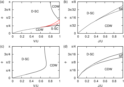
Figure 4: (Color online) Phase diagrams at quarter-filling with $t=1$, $t_{\perp}=0.01$, $U=2$ and (a) $N=2$, $J=0$ (b) $N=2$, $V=0$ (c) $N=10$, $J=0$ (d) $N=10$, $V=0$. Dashed lines indicate where $\phi$ is small enough so that some interactions not considered are larger than some which are considered.

The region in Fig. 4(a) which is marked in red describes a region of unusual scaling. The phase in this region is either D-SC or S-SC, with the D-SC to S-SC phase transition running approximately through the center. Each phase is characterized by a unique set of RG solutions of the eight coupling constants and generally, while renormalizing, the coupling constants flow gradually towards this final final solution. In the red region the coupling constants do not initially flow towards either a D-SC or S-SC solution but instead towards a solution typical of the D-SC to S-SC phase transition. This scaling behavior continues as $\ell$ increases, but at some point there is a sudden change and the RG will flow rapidly to either a D-SC or S-SC solution. This scaling behavior is typical when extremely close to a phase transition, but it is not usually observed in regions as large as the red region in Fig. 4(a). It is quite possible that this region could be mistaken for a TLL phase, as we shall explain in more detail in the next section. Note that this region is very close to $\phi=\pi/2$ so it may explain the TLL observations in LPB. Wang06

IV Tomanaga-Luttinger liquid

In the previous section we constructed various phase diagrams while assuming physically realistic conditions, yet did not observe a TLL. In this section we look more closely at what is required for the RG equations to flow towards a TLL solution. We simplify the problem a little by considering a two-leg ladder with the interaction cutoff $N=1$. Note that in this limit, the zigzag angle $\phi$ does not affect the initial values of the couplings and thus can be ignored. This model was discussed in Ref. Wang06, to describe LPB and solved using RG flow equations equivalent to the ones used here. Note that one of the key features for TLL is the critical exponent $\alpha$ of the single-particle density of states. Quasi-particle excitations are not found in a zero-temperature TLL so the single-particle density of states $\rho(\epsilon)$ at energy $\epsilon$ should be suppressed near the Fermi energy $\epsilon_{F}$. This suppression is expected to follow a power law $\rho(\epsilon)\propto|\epsilon-\epsilon_{F}|^{\alpha}$ for some positive constant $\alpha$ as the temperature approaches zero. Voit94

In Ref. Wang06, , it was argued, both experimentally and theoretically, that the nature of the critical exponent $\alpha$ indicates that LPB has a TLL phase. A remarkable agreement was found between the experimental value of $\alpha$ and the theoretical value obtained from the RG solutions, but what electron-electron interactions would provided the required initial conditions of the RG equations were not stated. Here we will discuss the electron-electron interactions which may support a TLL in a LPB-like two-leg ladder.

We can evaluate $\alpha$ numerically at different temperatures from the coupled RG equations. Note that the the temperature scales as $T=T_{0}e^{-\ell}$ under RG transformations, where $T_{0}$ is the initial (bare) temperature. Therefore, when calculating the couplings’ flow with the logarithmic length scale $\ell$, we can compute the critical exponent $\alpha$ at different temperatures. It is known that the exponent takes the form,

$$\alpha=(K_{\rho+}+K_{\rho+}^{-1}+K_{\rho-}+K_{\rho-}^{-1}-4)/8.$$ (24)

If it approaches a constant during the RG analysis we have a hint of TLL behaviour. Wang06 For convenience we separate this critical exponent into two parts, $\alpha=\alpha_{+}+\alpha_{-}$ where

$$\alpha_{\pm}=(K_{\rho\pm}+K_{\rho\pm}^{-1}-2)/8.$$ (25)

As has been discussed previously, the couplings in front of the sinusoidal terms in Eq. (15) determine the energy gaps and thus the nature of the phase. If none of these couplings become relevant under RG transformation, the ground state is gapless and is characterize by the so-called Luttinger parameters $K_{\rho\pm}$ and $K_{\sigma\pm}$ in the charge and spin sectors. In this case only the first line of Eq. (15) remains, which corresponds to the TLL Hamiltonian. vonDelft98 If at least one of the coefficients of the sinusoidal terms does not flow to zero we have any one of the Mott, SC, or density wave states discussed above. Three couplings, $b^{\rho}_{qq}$ with $q=1,2$ and $f^{\rho}_{12}$, are not coefficients of sinusoidal terms so need not vanish in a TLL. From the RG equations it can be seen that these three couplings will remain roughly constant when, and only when, all the other gap-inducing couplings are irrelevant. Lin98 ; Chang05 Furthermore, only these three couplings appear in Eq. (24) which defines $\alpha$. This is in agreement with what we have already stated about a TLL, i.e. the RG solution of $\alpha$ must flow to a constant value.

We can make some comments about the general behavior of $\alpha$. From the RG flow equations we determine that $b^{\rho}_{qq}$ always decreases, but $f^{\rho}_{12}$ always increases. In fact, $b^{\rho}_{11}+b^{\rho}_{22}+2f^{\rho}_{12}$ remains constant in RG flows. Therefore $K_{\rho+}$ must be a constant and $K_{\rho-}$ always increases. This implies $\alpha_{+}$ is a constant and the flow of the exponent $\alpha$ is essentially determined by $\alpha_{-}$. The minimum of $\alpha$ will be when $\alpha=\alpha_{+}$, which corresponds to $\alpha_{-}=0$ and $K_{\rho-}=1$, or equivalently $b^{\rho}_{11}+b^{\rho}_{22}=2f^{\rho}_{12}$. When $K_{\rho-}<1$ (or $b^{\rho}_{11}+b^{\rho}_{22}>2f^{\rho}_{12}$) $\alpha_{-}$ will decrease, as must $\alpha$, but when $K_{\rho-}>1$ both $\alpha_{-}$ and $\alpha$ will increase. The point $b^{\rho}_{11}+b^{\rho}_{22}=2f^{\rho}_{12}$ is more significant that just the turning point of $\alpha$. The RG flow equations indicate that once this point has been reached our system cannot be a TLL and $\alpha$ will increase at an increasing rate. So, once $b^{\rho}_{11}+b^{\rho}_{22}<2f^{\rho}_{12}$, or equivalently $K_{\rho-}>1$, in the RG flows, the TLL phase is unstable and some energy gaps will appear. However, it is important to emphasize that with $b^{\rho}_{11}+b^{\rho}_{22}>2f^{\rho}_{12}$ satisfied we may have a TLL but it is not guaranteed.

Returning to our specific example of LPB, we again assume quarter-filling and set $t=1$, $t_{\perp}=0.01$. In this case $k_{F1},k_{F2}\sim\pi/4$. Using the initial conditions in Eqs. (12) and (13) it can be shown that the condition $b^{\rho}_{11}+b^{\rho}_{22}>2f^{\rho}_{12}$ is equivalent to

$$J_{\perp 0}+2\sum_{n=1}^{N/2}(-1)^{n}J_{\perp 2n}<-{\textstyle{\frac{4}{3}}}[V_{\perp 0}+2\sum_{n=1}^{N/2}(-1)^{n}V_{\perp 2n}].$$ (26)

In order to compare our results with Ref. Wang06, we only consider the charge interactions $V_{\perp}=V_{\perp 0}$, $V_{d}=V_{\perp 1}$, $V_{\parallel}=V_{\parallel 1}$ and the spin interactions $J_{\perp}=J_{\perp 0}$, and $J_{\parallel}=J_{\parallel 1}$ which corresponds to a cutoff $N=1$, and so the necessary but not sufficient condition for a TLL reduces to $J_{\perp}<-{\textstyle{\frac{4}{3}}}V_{\perp}$. We wish to restrict ourselves to physically possible cases so we must have $V_{\perp}\geq 0$ and therefore the spin interaction across rungs $J_{\perp}$ must be negative, implying ferromagnetic exchange coupling. In Fig. 5 we present four phase diagrams, all of which show a LL may be obtained for negative $J_{\perp}$. In all cases the condition $J_{\perp}<-{\textstyle{\frac{4}{3}}}V_{\perp}$ is satisfied when we have a TLL, but clearly it does not imply that we must have a TLL.

Figure 5: Phase diagrams at quarter-filling with $t=1$, $t_{\perp}=0.01$, $U=2$ and (a) $V_{\parallel}=V_{d}=J_{\parallel}=0$, (b) $V_{\perp}=V_{d}=J_{\parallel}=0$, (c) $V_{\perp}=V_{\parallel}=J_{\parallel}=0$, (d) $V_{\perp}=V_{\parallel}=V_{d}=0$

If we wish to choose initial conditions which will enable the RG flow of $\alpha$ to closely resemble the experimental data in Ref. Wang06, then even greater restrictions are placed on $J_{\perp}$. As the interaction strengths are unknown we must attempt to make a reasonable guess. We set $U=2$ and to make the numerical search practical we set $V_{\perp}=V_{\parallel}$. Then, we fit the experimental data by varying the bare values of the charge interactions $V_{\perp},V_{d}$ and the spin interactions $J_{\perp},J_{\parallel}$. According to experimental data Wang06 $0.6\lesssim\alpha<1$, with $\alpha=1$ corresponding to the highest temperature measurement. So, we set $\alpha_{+}=0.6$ as this marks the minimum of $\alpha$ and this sets $K_{\rho+}=0.15$. The maximum value is set to $\alpha(T_{0})=1$ so $\alpha_{-}(T_{0})=\alpha(T_{0})-\alpha_{+}=0.4$ and $K_{\rho-}(\ell=0)=0.20$. These conditions determine the initial values of $b^{\rho}_{11}+b^{\rho}_{22}\pm 2f^{\rho}_{12}$ which in turn determine $V_{\perp},V_{d}$ for a given choice of $J_{\perp},J_{\parallel}$. The RG flow of $\alpha$ which corresponds to the experimental data is shown in Fig. 6, with the initial temperate $T_{0}=300$ K. We find that a TLL with $0.6\lesssim\alpha<1$ is only obtained when $J_{\perp}$ is quite large (significantly larger than $U$) and negative, which is unrealistic for LPB. This does not mean that a TLL phase is impossible for LPB as we must bear in mind that these simple one-loop RG solutions are not expected to be quantitatively correct and should really only be used for qualitative analysis. Consequently, forcing the theoretical value of $\alpha$ to fit the experimental data is not recommended and will not give a good prediction of the interactions in the lattice.

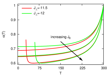
Figure 6: (Color online) The critical exponent $\alpha$ at quarter-filling with $t=1$, $t_{\perp}=0.01$, $U=2$,$V_{\parallel}=V_{\perp}$ and $J_{\parallel}=(1+2j)$ with $j=0,1,2$. While the arrow indicates increasing $J_{\parallel}$ for the curves show here, it does not indicate a general trend. The lowest red line and the lowest green line diverge so are not TLL, while the other four lines approach constant values and imply a TLL state.

Despite the limitations of this RG method it has had some success in predicting phases of various systems. Rather than attempt to obtain the exact experimental values of $\alpha$ one could simply try to replicate the line shape of $\alpha$ as the temperature decreases. In Fig. 7(a) we show that the general line shape observed in experiments is obtainable when $J_{\perp}$ is not particularly large, although it must be ferromagnetic because we are still bound by the condition $J_{\perp}<-{\textstyle{\frac{4}{3}}}V_{\perp}$ if we wish to have a TLL. In Fig. 7(b) we show that when we do not have a TLL $\alpha$ may still adopt a variety of line shapes, some of which strongly resemble a TLL as their turning point is very close to $T=0$, in particular the $J_{\parallel}=-J_{\perp}=1/2$ case. Also, by rescaling the interaction strengths it is possible to rescale almost any $\alpha$ to have a very low temperature turning point.

If we rescale all interactions by the same factor $R$ so that $(U,J_{n\parallel},J_{n\perp},V_{n\parallel},V_{n\perp})\rightarrow(U,J_{n\parallel},J_{n\perp},V_{n\parallel},V_{n\perp})/R$ then, because the initial couplings are linear in the interactions we can define a new set of couplings $\tilde{g}_{i}$ in terms of these rescaled interactions, $g_{i}(\ell=0)=R\tilde{g}_{i}(\ell=0)$. Rescaling the RG flow equations in the same way gives $d\tilde{g}_{i}/d\tilde{\ell}=\sum_{jk}A^{jk}_{i}\tilde{g}_{j}\tilde{g}_{k}$ where $\tilde{\ell}=R\ell$ and because it is the ratios $(J_{n\parallel},J_{n\perp},V_{n\parallel},V_{n\perp})/U$ which essentially determine the phase both $g_{i}$ and $\tilde{g}_{i}$ should flow towards the same solution and eventually describe the same phase. However, this does not mean they will have the same scaling. The rescaled temperature is $\tilde{T}=T_{0}e^{-\tilde{l}}$ and so $\tilde{T}=T_{0}(T/T_{0})^{-R}$ and therefore, by choosing an appropriate $R$ we may rescale $\alpha$ so that its turning point is very close to $T=0$ and the phase may closely resemble a TLL over a large temperature scale. For example, the $J_{\parallel}=-J_{\perp}=4$ curve in Fig. 7(b) has a turning point at $T$=115 K, but if we choose $R=2$ we rescale to $U=1$ and $J_{\parallel}=-J_{\perp}=2$ which rescales the turning point of $\alpha$ to $T=44$ K. Similarly, if we choose $R=4$ we obtain a turning point at $T=6.4$ K.

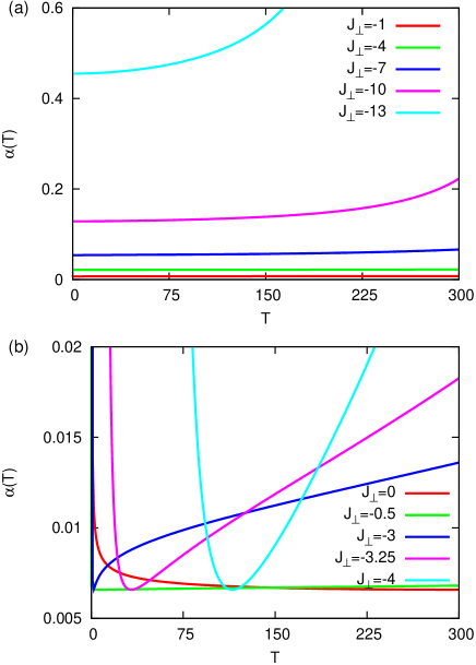
Figure 7: (Color online) The critical exponent $\alpha$ at quarter-filling with $t=1$, $t_{\perp}=0.01$, $U=2$ and (a) $J_{\parallel}=V_{\perp}=V_{\parallel}=V_{d}=0$ resulting in a TLL, (b) $J_{\parallel}=-J_{\perp}$, $V_{\perp}=V_{\parallel}=V_{d}=0$ not resulting in a TLL.

In Fig (8) we show the RG flow of the couplings for the $U=2$, $J_{\parallel}=-J_{\perp}=1/2$ case. These couplings mostly behave very much like one would expect in a TLL, with $f^{\sigma}_{12}$, $b^{\sigma}_{12}$ and $b^{\sigma}_{11}$ approaching zero while $b^{\rho}_{11}$ and $f^{\rho}_{12}$ are fairly constant, resulting in a fairly constant $\alpha$ over a large temperature range. Only $b^{\rho}_{12}$ does not have typical TLL behavior as it does not approach zero. Because of this the RG eventually flows away from typical TLL behavior and the couplings become large, in this case flowing towards a typical D-SC solution. In the previous section it was mentioned that the region outlined in red in Fig. 4(a) is not a TLL, but may be mistaken for one. This is because these couplings scale similarly to the ones shown in Fig (8), specifically $b^{\rho}_{11}$ and $f^{\rho}_{12}$ (and therefore $\alpha$) remain fairly constant over a significant $\ell$ range but at some point they make a rapid change and approach values typical of a superconductor. As the experimental data of LPB also hints at an increase in the critical exponent $\alpha$ near $T=0$, Wang06 it cannot be ruled out that the observed scaling is indeed a close crossover from TLL-like behavior to some superconducting or density wave phase near zero temperature.

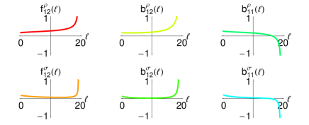
Figure 8: (Color online) The renormalized coupling constants (rescaled by $4\pi v_{q}$) at quarter-filling with $t=1$, $t_{\perp}=0.01$, $U=2$, $J_{\parallel}=-J_{\perp}=0.5$ and $V_{\parallel,\perp,d}=0$.

V Conclusions

We have derived a Hamiltonian for a two-leg ladder which allows consideration of generic short-range charge and spin interactions. One can choose the interactions to extend only to nearest neighbors, or one can choose to have interactions which extend across several lattice sites. When increasing the range of the interactions the number of variables inevitably increases. Rather than considering each interaction strength as an independent variable and dealing with all the associated problems, we can simply assume that the interactions are inversely proportional to the distance between lattice sites, thus keeping the number of parameters to a minimum. Using this method we were able to solve the RG solutions for any number of interactions while only needing three variables, $U$, $V$ and $J$, to describe the electron-electron interactions.

The Hamiltonian derived here is applicable to several different materials, and not just those materials like LPB which have an obvious ladder structure. Carbon nanotubes, for example, have an hexagonal lattice structure which may be mapped onto a two-leg ladder, and results obtained from two-leg ladder RG equations have been applied to carbon nanotubes with nearest-neighbor interactions. Bunder08 However, carbon nanotubes are known to support long-range interactions so the Hamiltonian presented here, with slight modifications, would provided a more accurate picture of the phases of a carbon nanotube.

Our RG analysis of LPB is somewhat limited because we have no experimental data which gives any clear indication of the charge and spin interaction strengths. It is important to note that this data should not be obtained indirectly by attempting to fit the experimental flow of the critical exponent $\alpha$ to numerical solutions of $\alpha$ obtained from the RG equations as these numerical solutions are not expected to be quantitatively accurate. Because of these limitations we are unable to make a definite statement concerning a TLL phase in LPB. The observed behavior may be a true TLL phase, or it may simply be a non-TLL phase which strongly resembles a TLL over a large temperature range. The power of these one-loop RG solutions is that they are relatively simple and tend to provide a qualitative description of the phase of the system. More quantitative accuracy may possibly be achieved from second-loop or higher order corrections. Tsuchiizu06

We acknowledge support from the National Science Council of Taiwan through grants NSC-96-2112-M-007-004 and NSC-97-2112-M-007-022-MY3 and also support from the National Center for Theoretical Sciences in Taiwan.

References

- (1) E. Dagotto and T. M. Rice, Science 271, 618 (1996).
- (2) S. Maekawa, Science 273, 1515 (1996).
- (3) D. Scalapino, Nature (London) 377, 12 (1995).
- (4) H. Mayaffre, P. Auban-Senzier, M. Nardone, D. Jérome, D. Poilblanc, C. Bourbonnais, U. Ammerahl, G. Dhalenne, A. Revcolevschi, Science 279, 345 (1998).
- (5) G. Blumberg, P. Littlewood, A. Gozar, B. S. Dennis, N. Motovama, H. Eisaki, and S. Uchida, Science 297, 584 (2002).
- (6) H.-H. Lin, L. Balents and P. A. Fisher, Phys. Rev. B 58, 1794 (1998).
- (7) J. O. Fjaerestad and J. B. Marston, Phys. Rev. B 65, 125106 (2002).
- (8) F. Wang, J. V. Alvarez, S.-K. Mo, J. W. Allen, G.-H. Gweon, J. He, R. Jin, D. Mandrus and H. Höchst, Phys. Rev. Lett. 96, 196403 (2006).
- (9) M. Tsuchiizu and A. Furusaki, Phys. Rev. B bf 66, 245106 (2002).
- (10) C. Wu, W. V. Liu and E. Fradkin, Phys. Rev. B 68, 115104 (2003).
- (11) M. Tsuchiizu and Y. Suzumura, Phys. Rev. B 72, 075121 (2005).
- (12) G. Y. Chitov, B. W. Ramakko and M. Azzouz, Phys. Rev. B 77, 224433 (2008).
- (13) Z. S. Popović and S. Satpathy, Phys. Rev. B 74 045117 (2006).
- (14) C. Brünger, F. F. Assaad, S. Capponi, F. Alet, D. N. Aristov and M. N. Kiselev, Phys. Rev. Lett. 100, 017202 (2008).
- (15) C. Kim, A. Y. Matsuura, Z.-X. Shen, N. Motoyama, H. Eisaki, S. Uchida, T. Tohyama, and S. Maekawa, Phys. Rev. Lett. 77 4054 (1996).
- (16) P. Segovia, D. Purdie, M. Hengsberger and Y. Baer, Nature 402, 504 (1999).
- (17) M. Bockrath, D. H. Cobden, J. Lu, A. G. Rinzler, R. E. Smalley, L. Balents and P. L. McEuen, Nature 397, 598 (1999).
- (18) H. Ishii, H. Kataura, H. Shiozawa, H. Yoshioka, H. Otsubo, Y. Takayama, T. Miyahara, S. Suzuki, Y. Achiba, M. Nakatake, T. Narimura, M. Higashiguchi, K. Shimada, H. Namatame and M. Taniguchi, Nature 426, 540 (2003).
- (19) M. Hilke, D. C. Tsui, M. Grayson, L. N. Pfeiffer and K. W. West, Phys. Rev. Lett. 87 186806 (2001).
- (20) X. G. Wen, Phys. Rev. B 41, 12838 (1990).
- (21) U. Ledermann, K. Le Hur and T. M. Rice, Phys. Rev. B 62, 16383 (2000).
- (22) J. von Delft and H. Schoeller, Ann. Phys. 7, 225 (1998).
- (23) M.-S. Chang, W. Chen and H.-H. Lin, Prog. Theor. Phys. 160, 79 (2005).
- (24) D. Jaksch and P. Zoller, Ann. Phys. 315, 52 (2005).
- (25) J. Voit, Rep. Prog. Phys. 57, 977 (1994).
- (26) J. E. Bunder and H.-H. Lin, Phys. Rev. B 78, 035401 (2008).
- (27) M. Tsuchiizu, Phys. Rev. B 74, 155109 (2006).