Quantitative analysis of clumps in the tidal tails of star clusters

Abstract

Tidal tails of star clusters are not homogeneous but show well defined clumps in observations as well as in numerical simulations. Recently an epicyclic theory for the formation of these clumps was presented. A quantitative analysis was still missing. We present a quantitative derivation of the angular momentum and energy distribution of escaping stars from a star cluster in the tidal field of the Milky Way and derive the connection to the position and width of the clumps. For the numerical realization we use star-by-star $N$-body simulations. We find a very good agreement of theory and models. We show that the radial offset of the tidal arms scales with the tidal radius, which is a function of cluster mass and the rotation curve at the cluster orbit. The mean radial offset is 2.77 times the tidal radius in the outer disc. Near the Galactic centre the circumstances are more complicated, but to lowest order the theory still applies. We have also measured the Jacobi energy distribution of bound stars and showed that there is a large fraction of stars (about 35%) above the critical Jacobi energy at all times, which can potentially leave the cluster. This is a hint that the mass loss is dominated by a self-regulating process of increasing Jacobi energy due to the weakening of the potential well of the star cluster, which is induced by the mass loss itself.

1 Introduction

Recently well-defined clumps were observed in the tidal tails of globular clusters by Leon et al. (2000) for NGC 6254 and Pal 12 and by Odenkirchen et al. (2001, 2003) for Pal 5. External perturbations like crossing of the galactic disc, peri-centre passage or near-encounters with other globular clusters were discussed as the source of the clumps (Capuzzo Dolcetta et al., 2005). In Capuzzo Dolcetta et al. (2005) the formation of these clumps in tidal tails of star clusters on eccentric orbits were confirmed by numerical studies. But the clumps occur also in the tidal tails of star clusters on circular orbits with no external push. Recently, Küpper et al. (2008) presented a theoretical explanation for the clump formation in a constant tidal field. It is essentially due to the epicyclic motion of the stars lost by the star cluster.

We present a quantitative analysis of the tidal tail structure for star clusters moving on a circular orbit in the galactic disc. The analysis is based on numerical simulations with realistic particle numbers including an initial mass function (IMF) and stellar evolution. We compare the results for star clusters at the solar circle and near the Galactic centre. Since the epicycle theory is a perturbation theory with respect to a circular orbit with constant tidal field, we cannot apply it for predictions of clump distances to the eccentric orbits of the observed globular clusters. On the other hand the observation of tidal tail clumps of open clusters in the galactic disc are hampered by the overwhelming number of field stars with similar properties. For an identification the contrast in density and velocity with respect to the field stars may be too small. Additionally the tidal tails may be destroyed quickly by the same gravitational scattering process, which is also responsible for the dynamical heating of the stellar disc. We discuss the observability further in Sect. 5.

In Section 2 we present the epicyclic theory for the stars in the tidal tails and the connection to the mass loss and the orbit of the star cluster. In Section 3 we present the numerical codes used and the properties of the star clusters. Section 4 contains the quantitative comparison of the numerical results with the theoretical predictions. In Section 5 we summarize our results.

2 Dynamics of escaping stars

In the first part of this section we derive the orbital properties of the stars in the tidal tails in terms of angular momentum and energy. Then we discuss the connection of mass loss with the Jacobi energy distribution of the stars. Finally the tidal tail properties are determined with respect to the star cluster orbit.

Classically the gravitational potential $\Phi_{\mathrm{g}}(R)$ and kinetic energy $\Omega^{2}R^{2}/2$ are approximated to second order in the variable $r=R-R_{0}$, which we will also use. For the determination of the tidal tail properties with respect to the star cluster orbit in Section 2.3 we switch to the Taylor expansion with respect to angular momentum (e.g. for $R_{0}(L)=\sqrt{L/\Omega(L)}$ equation A), because $L$ is a constant of motion for the tidal tail stars and easily measurable.

2.1 Motion of tidal tail stars

As soon as the gravitational potential of the star cluster is negligible, stars in the tidal tails move in the axisymmetric potential of the Galaxy. The orbits can be calculated in the epicyclic approximation (see Küpper et al. (2008) for a recent application to tidal tail structure). The radial offset of the epicyclic motion relative to the orbit of the star cluster is first order in the angular momentum. The radial amplitude depends on the energy excess, which is of second order.

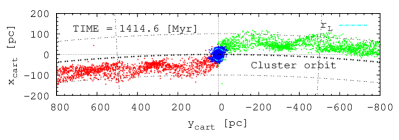
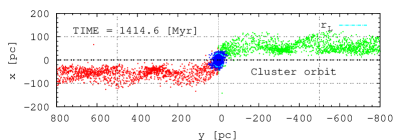
Figure 1: Visualization of the local cartesian (top) and local cylindrical coordinates (bottom) for the snapshot at t=1.414 Gyr of model 10, where the origin is moved from the galactic centre to the star cluster centre. Black (blue) dots are the bound stars, dark grey dots to the left (red) are the stars of the leading arm and light grey dots to the right (green) are the stars in the trailing arm. The light dashed (cyan) circle marks the tidal radius.

Since the tidal tails may extend over a considerable range in azimuth, we use polar coordinates $R,\varphi,z$ with origin at the galactic centre. Fig. 1 shows the effect of switching from local cartesian ($x_{\mathrm{cart}},y_{\mathrm{cart}}$) to local polar ($x,y$) coordinates. We restrict the investigation to orbits in the galactic plane $z=0$, but a generalization is straightforward. Energy $E$ and the z-component of angular momentum $L=L_{z}$ are isolating integrals of motion in the axisymmetric potential of the Galaxy. The motion is a 2-dimensional harmonic oscillation with the epicyclic frequency $\kappa$ (see equation 38). We use the normalized epicyclic frequency $\beta=\kappa/\Omega$. The ’epicentre’ (guiding centre) of the oscillation is described by

$$(R,\varphi)_{0}=(R_{0},\Omega_{0}t)$$ (1)

where $\Omega(R)$ is the angular frequency of the galactic rotation and $\Omega_{0}=\Omega(R_{0})$. $R_{0}$ is determined by the angular momentum of the star via

$$L=L_{0}=\Omega_{0}R_{0}^{2}$$ (2)

In one epicyclic period $T=2\pi/\kappa_{0}$ the epicentre moves along the circle with radius $R_{0}$ by

$$D_{0}(T)=\frac{2\pi}{\kappa_{0}}\Omega_{0}R_{0}=\frac{2\pi}{\beta_{0}}R_{0}$$ (3)

The energy of the star determines the amplitude of the oscillation. At the apo- and pericentre $R_{\mathrm{m}}$, where the radial motion vanishes, it can be written as

$$E=\Phi_{\mathrm{g}}(R_{\mathrm{m}})+\frac{L_{0}^{2}}{2R_{\mathrm{m}}^{2}}$$ (4)

with the galactic potential $\Phi_{\mathrm{g}}(R)$. Relative to the circular motion with

$$E_{0}=\Phi_{\mathrm{g}}(R_{0})+\frac{L_{0}^{2}}{2R_{0}^{2}}$$ (5)

the radial amplitude $r_{\mathrm{m}}=R_{\mathrm{m}}-R_{0}$ is determined by the energy excess

$$\Delta E=E-E_{0}=\Phi_{\mathrm{g}}(R_{\mathrm{m}})-\Phi_{\mathrm{g}}(R_{0})+\frac{L_{0}^{2}}{2}\left(\frac{1}{R_{\mathrm{m}}^{2}}-\frac{1}{R_{0}^{2}}\right)$$ (6)

To second order in $r$ (see App. A) we find for the radial amplitude $r_{\mathrm{m}}$ and peri/apocentre position $R_{\mathrm{m}}$

$$R_{\mathrm{m}} = R_{0}\pm r_{\mathrm{m}}=R_{0}\pm\frac{\sqrt{2\Delta E}}{\beta_{0}\Omega_{0}}$$ (7)

Note that the epicentre is determined by the angular momentum $L$ of the star and the radial amplitude by the energy excess $\Delta E$.

The amplitude in tangential direction is

$$y_{\mathrm{m}}=R_{0}\Delta\varphi_{\mathrm{m}}=\frac{2}{\beta_{0}}r_{\mathrm{m}}$$ (8)

The epicyclic ellipse is elongated into the radial direction, because $1\leq\beta\leq 2$ for reasonable rotation curves.

2.2 Mass loss of the star cluster

We investigate the mass loss of a star cluster on a circular orbit with $R_{\mathrm{C}},\Omega_{\mathrm{C}}$ in the tidal field of the Galaxy. The orbit of the cluster is offset to the epicentres $R_{0},\Omega_{0}$ of the stars in the tidal tails. The differential rotation results in the elongation of the tidal tails.

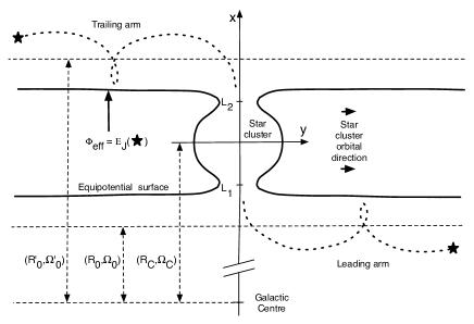
Figure 2: Top: Effective potential of a star cluster in the corotating frame. L1 and L2 are the Lagrange points. Bottom: Sketch of escaping stars in the effective potential of a star cluster through the Lagrange points L1 and L2.

As long as the stars are influenced by the gravitational potential of the cluster, it is appropriate to use a reference frame corotating with the star cluster. We use cylindrical coordinates $(R,\varphi)$ corotating with the star cluster and with the origin at the galactic centre. The angular speed is $\Omega_{\mathrm{C}}$ and the star cluster centre is at $(R_{\mathrm{C}},\varphi=0)$. Then we shift the origin to the star cluster centre and use a local cylindrical coordinate system with $x=R-R_{\mathrm{C}}$ and $y=R\varphi$ (for an illustration see figure  1).

In the corotating system we set the zero point of the galactic potential $\Phi_{g}$ such that the effective potential $\Phi_{\mathrm{g,eff}}(R_{\mathrm{C}})=\Phi_{g}-\Omega_{\mathrm{C}}^{2}R_{\mathrm{C}}^{2}/2=0$ vanishes at $R_{\mathrm{C}}$. We get

$$\Phi_{\mathrm{eff}}=\Phi_{\mathrm{cl}}+\Phi_{\mathrm{g}}-\Phi_{\mathrm{g}}(R_{\mathrm{C}})-\frac{\Omega_{\mathrm{C}}^{2}}{2}(R^{2}-R_{\mathrm{C}}^{2})$$ (9)

The Jacobi energy $E_{\mathrm{J}}$, which is the only known constant of motion (Binney & Tremaine, 1987), is given by

$$E_{\mathrm{J}}=E-\Omega_{\mathrm{C}}L=\Phi_{\mathrm{eff}}+\frac{v^{2}}{2}$$ (10)

with velocity $v$ in the corotating rest frame. The Jacobi energy of the cluster motion in the galactic potential vanishs. The effective potential has saddle points at the inner and outer Lagrange points L1/L2 (Fig. 2), where the stars are leaking out. All stars with Jacobi energy exceeding the critical value $E_{\mathrm{J,crit}}=\Phi_{\mathrm{eff}}(L1/L2)$ can in principle leave the cluster.

For the effective potential we get at $y=0$

$$\Phi_{\mathrm{eff}}(x,0)=\frac{\beta_{\mathrm{C}}^{2}-4}{2}\Omega_{\mathrm{C}}^{2}x^{2}+\Phi_{\mathrm{cl}}(x,0)$$ (11)

The tidal radius $r_{\mathrm{L}}$ is given by the distance of the Lagrange points to the cluster centre. It is determined by

$$0 = \frac{\mbox{\rm d}\Phi_{\mathrm{eff}}}{\mbox{\rm d}x}=\Omega_{\mathrm{C}}^{2}(\beta_{\mathrm{C}}^{2}-4)r_{\mathrm{L}}\pm\frac{GM_{\mathrm{cl}}(r_{\mathrm{L}})}{r_{\mathrm{L}}^{2}}$$ (12)

where $M_{\mathrm{cl}}(r_{\mathrm{L}})$ is the cluster mass enclosed in $|r_{\mathrm{L}}|$. We find the well known equation for the tidal radius

$$r_{\mathrm{L}}^{3}=\frac{\pm GM_{\mathrm{cl}}}{(4-\beta_{\mathrm{C}}^{2})\Omega_{\mathrm{C}}^{2}}$$ (13)

where we assumed that the full cluster mass is enclosed in $|r_{\mathrm{L}}|$. The effective potential at the Lagrange points is

$$\Phi_{\mathrm{eff}}(|r_{\mathrm{L}}|,0)=E_{\mathrm{J,crit}}=-\frac{3}{2}(4-\beta_{\mathrm{C}}^{2})\Omega_{\mathrm{C}}^{2}r_{\mathrm{L}}^{2}=-\frac{3}{2}\frac{GM_{\mathrm{cl}}}{|r_{\mathrm{L}}|}$$ (14)

The last expression shows that the contribution from the star cluster potential is twice that of the effective potential of the Galaxy.

A star starting near L1 or L2 with velocity $v_{\mathrm{L}}$ escapes at constant Jacobi energy but with changing energy and angular momentum until the cluster potential can be neglected. Then the position ($x,y$) and velocity $v=(v_{\mathrm{r}},v_{\mathrm{t}})$ in the tidal tail are related to ($r_{\mathrm{L}},0$) and $v_{\mathrm{L}}$ by

$$E_{\mathrm{J}}=\Phi_{\mathrm{eff}}(r_{\mathrm{L}},0)+\frac{v_{\mathrm{L}}^{2}}{2}=\Phi_{\mathrm{g,eff}}(x)+\frac{v^{2}}{2}$$ (15)

leading to

$$x^{2}=3r_{\mathrm{L}}^{2}+\frac{\Delta(v^{2})}{(4-\beta_{\mathrm{C}}^{2})\Omega_{\mathrm{C}}^{2}}$$ (16)

or

$$\frac{x^{2}}{r_{\mathrm{L}}^{2}}=3+\frac{\Delta(v^{2})}{GM_{\mathrm{cl}}/|r_{\mathrm{L}}|}$$ (17)

with $\Delta(v^{2})=v^{2}-v_{\mathrm{L}}^{2}$. Stars moving along the equipotential surface ($\Delta(v^{2})=0$) yield as initial position $x=\sqrt{3}r_{\mathrm{L}}$ and initial velocity essentially tangential $v_{\mathrm{t}}\approx v_{\mathrm{L}}$. This approximation fits well with the radial position of the equipotential surface through L1/L2 at large distances from the cluster in Fig. 2. Stars moving radially gain kinetic energy ($\Delta v^{2}>0$) resulting in a larger $x$ and stars starting tangentially loose kinetic energy ($\Delta v^{2}<0$) leading to a smaller $x$.

For a continuous mass loss until dissolution it is necessary that the Jacobi energy of bound stars is lifted above the critical value $E_{\mathrm{J,crit}}$, which increases due to the mass loss. There are two physical effects, which are responsible for a continuous mass loss of the cluster. The first one is triggered by the mass loss of the cluster itself. Mass loss on a timescale large compared to the dynamical time of the cluster leads to an increase of $E_{\mathrm{J}}$ of the bound stars by

$$\frac{\mbox{\rm d}E_{\mathrm{J}}}{\mbox{\rm d}t}=\frac{\delta\Phi_{\mathrm{cl}}}{\delta t}\propto\dot{M}_{\mathrm{cl}}$$ (18)

But the critical value $E_{\mathrm{J,crit}}$ increases more slowly, because the tidal radius decreases with decreasing mass

$$\frac{\mbox{\rm d}\Phi_{\mathrm{eff}}(r_{\mathrm{L}},0)}{\mbox{\rm d}t}\propto\dot{M}_{\mathrm{cl}}^{2/3}$$ (19)

Initiated by mass loss due to stellar evolution or by a few stars above $E_{\mathrm{J,crit}}$ mass loss will continue by stars lifted above the critical value.

The second process is dynamical evolution of the cluster due to 2-body encounters. With the relaxation timescale stars are scattered above $E_{\mathrm{J,crit}}$ and can leave the cluster. The relative importance of the two effects depend on the mass, number of stars and the structure of the cluster.

2.3 Dynamic parameters of tidal tail stars

Since the orbits are epicycles perturbed by the acceleration of the cluster, the connection of the initial position and velocity $(r_{\mathrm{L}},v_{\mathrm{L}})$ to $(x,v)$ at a later time, when the cluster potential can be neglected, is very complicated. Here we are interested in the statistics of initial and final properties of the escaping stars.

For the transition from bound stars to escaped stars, we need to combine the motion in the frame corotating with the cluster $R_{\mathrm{C}},\Omega_{\mathrm{C}}$ and that in the non-rotating reference frame, where we derived the properties of the epicycles around $R_{0},\Omega_{0}$. For measuring the shape and kinematics of the tidal tails we stay in the corotating rest frame centered at the cluster. Therefore we transform the epicyclic motion to the corotating frame with respect to $R_{\mathrm{C}},\Omega_{\mathrm{C}}$.

The radial offset $\Delta R_{0}=R_{0}-R_{\mathrm{C}}$ of the epicentre of a star is determined by the angular momentum difference $\Delta L=L-L_{\mathrm{C}}$ (see equation A). Here we need only the first order term of $\Delta R_{0}$ in $\Delta L$, which is

$$\frac{\Delta R_{0}}{R_{\mathrm{C}}} = \frac{2}{\beta_{\mathrm{C}}^{2}}\frac{\Delta L}{L_{\mathrm{C}}}=\frac{2}{\beta_{\mathrm{C}}^{2}R_{\mathrm{C}}}\left(2x+\frac{v_{\mathrm{t}}}{\Omega_{\mathrm{C}}}\right)$$ (20)

Since the epicycles are counterrotating with respect to the disc rotation, the relative velocity in the tidal tails is smallest at the pericentres (with respect to the cluster motion). These are the locations where the clumps occur. The tangential distance $y_{0}(T)$ of the pericentres in the corotating frame are determined by the shear flow of the epicentre motion. The period is $T=2\pi/\kappa_{0}$ leading to

$$y_{0}(T) = \frac{2\pi}{\kappa_{0}}R_{0}\left(\Omega_{0}-\Omega_{\mathrm{C}}\right)=\frac{2\pi}{\beta_{\mathrm{C}}}\frac{R_{\mathrm{C}}}{\Omega_{\mathrm{C}}}\Omega_{\mathrm{C}}^{\prime}\Delta R_{0}$$ (21)

$$= \frac{2\pi}{\beta_{\mathrm{C}}}\frac{\beta_{\mathrm{C}}^{2}-4}{2}\Delta R_{0}=\frac{2\pi}{\beta_{\mathrm{C}}}\frac{\beta_{\mathrm{C}}^{2}-4}{\beta_{\mathrm{C}}^{2}}\frac{\Delta L}{L_{\mathrm{C}}}R_{\mathrm{C}}$$

$$= \frac{4\pi}{\beta_{\mathrm{C}}}\frac{\beta_{\mathrm{C}}^{2}-4}{\beta_{\mathrm{C}}^{2}}\left(x+\frac{v_{\mathrm{t}}}{2\Omega_{\mathrm{C}}}\right)$$

For the special case of $x=r_{\mathrm{L}}$ and $v_{\mathrm{t}}=0$ we recover the equation given in Küpper et al. (2008). The spread in $\Delta L$ of the escaping stars leads to a corresponding tangential width of the first clump. In the succeeding clumps the tangential spread increases linearly and quickly smears out the pericentre positions over a whole period of $y_{0}(T)$.

The radial spread of the tidal tail stars is determined by the combined spread in $\Delta R_{0}$ and in the amplitudes $r_{\mathrm{m}}$. The amplitudes are determined by the second order terms in the energy excess of the stars with respect to the epicentre energy $E_{0}$. Relative to the cluster center energy $E_{\mathrm{C}}=\Phi_{\mathrm{g}}(R_{\mathrm{C}})+\Omega_{\mathrm{C}}^{2}R_{\mathrm{C}}^{2}/2$ and with the help of equation 5 we get for the energy difference of the epicentre

$$\Delta E_{0} = E_{0}-E_{\mathrm{C}}=\Omega_{\mathrm{C}}\Delta L-\frac{4-\beta_{\mathrm{C}}^{2}}{2\beta_{\mathrm{C}}^{2}}\frac{\Omega_{\mathrm{C}}}{L_{\mathrm{C}}}\Delta L^{2}$$ (23)

The amplitude of the epicycle is determined by the energy excess with respect to the epicentre energy $E_{0}$ and can be calculated using the Jacobi energy of the star

$$E_{\mathrm{J}} = \Phi_{\mathrm{g,eff}}(R_{\mathrm{C}}+x)+\frac{v^{2}}{2}=-\frac{4-\beta_{\mathrm{C}}^{2}}{2}\Omega_{\mathrm{C}}^{2}x^{2}+\frac{v^{2}}{2}$$ (24)

(taking into account the zero-point $\Phi_{\mathrm{g,eff}}(R_{\mathrm{C}})=0$) and equation 23 leading to

$$\Delta E = E-E_{0}=E_{\mathrm{J}}+\Omega_{\mathrm{C}}\Delta L-\Delta E_{0}$$ (25)

$$= E_{\mathrm{J}}+\Omega_{\mathrm{C}}L_{\mathrm{C}}\frac{4-\beta_{\mathrm{C}}^{2}}{2\beta_{\mathrm{C}}^{2}}\frac{\Delta L^{2}}{L_{\mathrm{C}}^{2}}$$ (26)

$$= E_{\mathrm{J}}+\Omega_{\mathrm{C}}^{2}\frac{\beta_{\mathrm{C}}^{2}}{2}\frac{4-\beta_{\mathrm{C}}^{2}}{4}\Delta R_{0}^{2}$$ (27)

Now the epicyclic amplitude $r_{\mathrm{m}}$ is determined by

$$r_{\mathrm{m}}^{2} = \frac{2\Delta E}{\beta_{\mathrm{C}}^{2}\Omega_{\mathrm{C}}^{2}}=\frac{4-\beta_{\mathrm{C}}^{2}}{4}\Delta R_{0}^{2}+\frac{2}{\beta_{\mathrm{C}}^{2}}\frac{E_{\mathrm{J}}}{\Omega_{\mathrm{C}}^{2}}$$

$$= \frac{2}{\beta_{\mathrm{C}}^{2}}\left[\frac{4-\beta_{\mathrm{C}}^{2}}{2\beta_{\mathrm{C}}^{2}}R_{\mathrm{C}}^{2}\frac{\Delta L^{2}}{L_{\mathrm{C}}^{2}}+\frac{E_{\mathrm{J}}}{\Omega_{\mathrm{C}}^{2}}\right]$$

The position of the apo/pericentre with respect to the cluster centre is given by

$$x_{\mathrm{m}} = R_{\mathrm{m}}-R_{\mathrm{C}}=\Delta R_{0}\pm r_{\mathrm{m}}$$ (29)

In terms of position $x$ and velocity $v_{\mathrm{r}},v_{\mathrm{t}}$ in the corotating frame the apo- and pericentre are given by

$$x_{\mathrm{m}} = \frac{1}{\beta_{\mathrm{C}}^{2}}\left(4x+\frac{2v_{\mathrm{t}}}{\Omega_{\mathrm{C}}}\right)$$

$$\pm\frac{1}{\beta_{\mathrm{C}}^{2}}\sqrt{\left(\left(4-\beta_{\mathrm{C}}^{2}\right)x-\frac{2v_{\mathrm{t}}}{\Omega_{\mathrm{C}}}\right)^{2}+\beta_{\mathrm{C}}^{2}\frac{v_{\mathrm{r}}^{2}}{\Omega_{\mathrm{C}}^{2}}}$$

If the star starts at peri/apo-centre (with no radial velocity $v_{\mathrm{r}}=0$) we find the corresponding apo/peri-centre by

$$v_{\mathrm{r}}=0: x_{\mathrm{m}}=\frac{1}{\beta_{\mathrm{C}}^{2}}\left(4x+\frac{2v_{\mathrm{t}}}{\Omega_{\mathrm{C}}}\pm\left|(4-\beta_{\mathrm{C}}^{2})x-\frac{2v_{\mathrm{t}}}{\Omega_{\mathrm{C}}}\right|\right)$$ (31)

In Küpper et al. (2008) the special case of $v_{\mathrm{r}}=v_{\mathrm{t}}=0$ and $x=r_{\mathrm{L}}$ was adopted, where the star has a Jacobi energy of $E_{\mathrm{J}}=-GM_{\mathrm{cl}}/(2r_{\mathrm{L}})=E_{\mathrm{J,crit}}/3$.

3 Numerical modeling

For the main investigation we used the direct $\phi$GRAPE $N$-body code to calculate the evolution of star clusters in an analytic Galaxy model. It is described in this section. For the case of a star cluster near the Galactic centre and for testing the reliability of the simulations we used a variant of the direct $N$-body6++ code, which is described in Section 4.4.

3.1 $\phi$GRAPE $N$-body code

For the high resolution direct $N$-body simulations at large galactocentric distances we used the specially developed $\phi$GRAPE code. The code itself and also the special GRAPE hardware is described in more detail in Harfst et al. (2007). Here we mention briefly the most important special features of the code. The program was already well tested with different $N$-body applications including the high resolution study of the dynamical evolution of the galactic centre with a binary (or single) Super-massive Black Hole (Berczik et al., 2005, 2006; Merritt et al., 2007). The same code was also recently used to study the shape parameters of a large set of rotating open star clusters (Kharchenko et al., 2008).

The program acronym $\phi$GRAPE means: Parallel Hermite Integration with GRAPE. The serial and parallel version of the program has been written from scratch in ANSI-C and uses the standard MPI library for communication. For the calculation of the star cluster dynamics in the galactic potential we use the parallel GRAPE systems built at the Astronomisches Rechen-Institut in Heidelberg, and at the Main Astronomical Observatory in Kiev.

The program uses the 4-th order Hermite integration scheme for the particles with hierarchical individual block timesteps, together with the parallel usage of GRAPE6a cards for the hardware calculation of the acceleration ${\bf a}$ and the first time derivative of the acceleration ${\bf\dot{{a}}}$ (this term is usually called ’jerk’ in the $N$-body community).

For the simulation of star clusters in the tidal field of the Galaxy an analytic external potential is added. We use an axi-symmetric three component model, where bulge, disc and halo are described by Plummer-Kuzmin models (Miyamoto & Nagai, 1975) with

$$\Phi(R,z)=-\frac{G\cdot M}{\sqrt{R^{2}+(a+\sqrt{b^{2}+z^{2}})^{2}}},$$ (32)

where $b$ is a measure of the core radius and $a$ a measure of the flattening.

Table 1: The list of galaxy component parameters. The first column gives the component, the second the mass, and the third and fourth the Plummer-Kuzmin parameters (equation 32).

Mass component	M [M⊙]	$a~{}[{\rm kpc}]$	$b~{}[{\rm kpc}]$
Bulge	$1.4\cdot 10^{10}$	0.0	0.3
Disk	$9.0\cdot 10^{10}$	3.3	0.3
Halo	$7.0\cdot 10^{11}$	0.0	25.0

For the parameters we use similar values as in Douphole & Colin (1995) with slightly corrected masses (see Table 1) to reproduce the observed Milky Way rotation curve in the solar neighbourhood. The rotation curve, the epicyclic frequency $\beta=\kappa/\Omega$ (normalized to the orbital frequency $\Omega$) and the logarithmic derivative $\beta^{\prime}=\mbox{\rm d}\beta/\mbox{\rm d}\ln R$ are shown in Fig. 3.

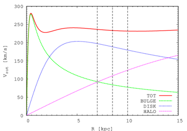
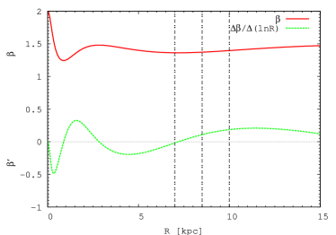
Figure 3: Top: Rotation curve of the Galaxy model and the contributions from bulge, disk and halo. Bottom: Epicyclic frequency parameter $\beta$ and the logarithmic derivative $\beta^{\prime}$. The vertical dashed lines mark the orbits of the star clusters selected for the investigation.

3.2 Initial conditions for the star cluster

The star clusters are modeled star by star using a Salpeter IMF (Salpeter, 1955) in the mass range of $0.08\leq m/\rm{M}_{\mathrm{\rm\sun}}\leq 8$. We include a simple model for stellar evolution from van den Hoek & Groenewegen (1997) and distribute the stellar mass loss uniformly over the metallicity dependent stellar lifetimes (Raiteri et al., 1996).

For the generation of the initial particle distribution and velocities we use a nonrotating King model with W${}_{0}=6.0$. In the $N$-body code the physical quantities are normalized by $G=M_{\mathrm{cl}}=1$ and total energy $E^{TOT}=-0.25$ as first introduced by Aarseth et al. (1974).

After generating the dimensionless parameters for the cluster data we set the different physical mass & half-mass radius parameters for the clusters. In general these two parameters can be set independently, but in order to reduce the number of free parameters we decided to use a physically motivated relation between initial mass and initial half-mass radius of the star clusters. For this purpose we use the extension of the well known mass vs. radius relation observed in molecular clouds and clumps in our Milky Way. For relevant references see the list of observational and theoretical papers Larson (1981); Solomon et al. (1987); Maloney (1990); Theis & Hensler (1993); Inoue & Kamaya (2000). Using such an approximation we can write down a scaling relation for our initial cluster size and mass. For fixing the size of the cluster we use the radius $r_{\mathrm{k}}$ containing 60% of the cluster mass (because this radius is approximately independent of rotation for future extension to rotating King models). We set

$$r_{\mathrm{k}}\approx 100\cdot\sqrt{\frac{M_{\mathrm{cl}}}{10^{6}\rm{M}_{\mathrm{\rm\sun}}}}~{}[{\rm pc}]$$ (33)

For the used three physical masses M_cl = 10³, 5$\cdot$10³ and 10⁴ [M${}_{\odot}]$ we get the corresponding radii $r_{\mathrm{k}}$ = 3.0, 7.0 and 10 [pc]. We do not adapt the ’tidal radius’ of the King models, where the density vanishes, to the tidal radius $r_{\mathrm{L}}$ of the galactic field. The starting point of the star cluster orbit is determined by the position in the galactic disk (0.0, $R_{\mathrm{C}}$, 0.0) with corresponding velocity (-$V_{\mathrm{C}}$, 0.0, 0.0) added to each star. The star cluster is nonrotating and has exactly the angular momentum $V_{\mathrm{C}}R^{2}_{\mathrm{C}}$. If $V_{\mathrm{C}}$ is exactly the circular velocity at $R_{\mathrm{C}}$, then the angular momentum corresponds to $L_{\mathrm{C}}$ of the circular orbit at $R_{\mathrm{C}}$. In contrast Fukushige et al. (2000) started with clusters in the corotating frame leading to an additional spin of the star cluster. For practical reasons the initial velocity was slightly smaller then the correponding circular speed at $R_{\mathrm{C}}$ by neglecting the decimal places. Therefore the star clusters in models 01–09 started at apo-centre and moved on an epicycle relative to the cluster epicentre motion. It turned out that the galactocentric distance variations of the cluster orbits are comparable to the tidal radii of the star clusters. Since the Jacobi energy is conserved only in a rest frame with constant angular speed, the origin of the coordinate system must be determined by the epicentre motion of the cluster and therefore the cluster centre is moving on an epicycle in that coordinate system. The main effect on the evolution of the tidal tails is an additional periodic force with the epicyclic frequency. In order to test the effect of this ’resonant forcing’ we set up model 10 which is on an exact circular orbit. The only difference to model 08 is the larger initial velocity by 0.3 km/s. The differences between these two models in the mass loss rate and in the position and strength of the tidal clumps are negligible. Therefore we use model 10 as the fiducial model for the detailed investigations. The other models are used to investigate the parameter dependences of the tidal tail structure. The cluster parameters of the models are listed in Table 2.

Table 2: The model parameters of all runs. Column 1 gives the number of the model, columns 2–4 are initial mass, number of particles and scale radius of the cluster, columns 5 and 6 are the initial position and velocity of the cluster, column 7 is the epicycle parameter at distance $R_{\mathrm{C}}$, column 8 is the initial Lagrange radius of the cluster.

#	Mcl [M⊙]	N	rk [pc]	RC [kpc]	VC [km/s]	$\beta$	rL [pc]
01	103	4040	3.0	7.0	236	1.363	12.08
02	103	4040	3.0	8.5	233	1.372	13.93
03	103	4040	3.0	10.0	231	1.396	15.78
04	5$\cdot$103	20202	7.0	7.0	236	1.363	20.66
05	5$\cdot$103	20202	7.0	8.5	233	1.372	23.82
06	5$\cdot$103	20202	7.0	10.0	231	1.396	26.98
07	104	40404	10.0	7.0	236	1.363	26.04
08	104	40404	10.0	8.5	233	1.372	30.00
09	104	40404	10.0	10.0	231	1.396	34.00
10	104	40404	10.0	8.5	233.297	1.372	30.00

4 Results

We discuss in detail the properties of model 10 on an exact circular orbit. In this case the origin of the corotating coordinate system is at the cluster centre. Firstly we analyze the mass loss and the Jacobi energy distribution of the bound stars. Then we determine Jacobi energy, angular momentum and energy excess of the stars in the tidal tails and compare the predictions with the clump positions and widths. Then we discuss the parameter dependence of the tidal tail structure. Finally we present a numerical simulation of a star cluster near the galactic centre to demonstrate the generality of the theory.

4.1 Cluster mass loss

There is no unique definition of bound stars for star clusters in tidal fields. The main reason is that many stars with Jacobi energy exceeding the critical value remain for a long time in the vicinity of the cluster. For determining the mass loss rate and for visualisation we use a rather conservative measurement by using an energy criterion in the comoving, but not corotating, reference system. We assume, that all particles which have a negative relative energy in the cluster potential are still bound to the cluster:

$$|E^{\mathrm{GRA}}_{\mathrm{i}}|_{\mathrm{cl}}>E^{\mathrm{KIN}}_{\mathrm{i}}.$$

An inspection of the particle distribution shows that this criterion coincides approximately with stars inside $|r_{\mathrm{L}}|$. On the basis of this criterium we create the list of particles denoted by ’dynamical’ cluster members. In Fig. 4 the difference in the Jacobi energy distribution of dynamical cluster members and of stars inside a sphere with radius $|r_{\mathrm{L}}|$ are shown. There are only small deviations at the high energy end.

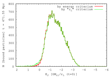
Figure 4: Jacobi energy distribution of dynamical cluster members and of stars inside a sphere with radius $|r_{\mathrm{L}}|$ at t=471 Myr of model 10. Note that lower values of $E_{\mathrm{J}}$ are to the right.

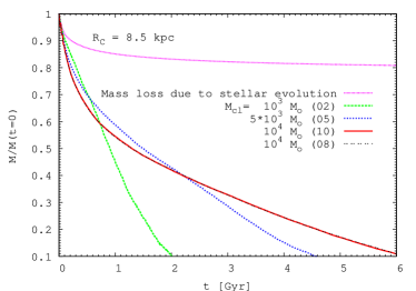
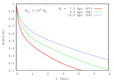
Figure 5: The time evolution of bound mass of the different models. Top: All models at distance $R_{\mathrm{C}}=8.5$ kpc. The top-most line shows the mass loss due to stellar evolution of all stars. Bottom: Models with initial mass $M_{\mathrm{cl}}=10^{4}\,\rm{M}_{\mathrm{\rm\sun}}$ at different distances to the galactic centre.

In Figure 5 we present the mass evolution of the star clusters. In the upper panel the models at $R_{\mathrm{C}}=8.5$ kpc are shown. Mass loss of model 08 at a slightly eccentric orbit shows a very small modulation compared to the corresponding model 10 on the exact circular orbit. The top line shows the mass loss of all stars due to stellar evolution for model 10. The bottom panel shows the mass evolution of models with initial mass $M_{\mathrm{cl}}=10^{4}\rm{M}_{\mathrm{\rm\sun}}$ at different galactocentric distances.

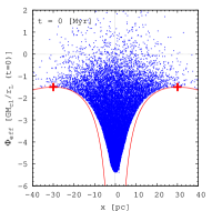
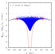
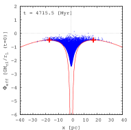
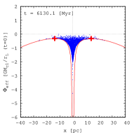
Figure 6: The effective potential of all bound particles for different times of model 10. The full (red) lines show the analytic approximation according to equation 11. The vertical tics show the position and energy of the Lagrange points $r_{\mathrm{L}}$.

Figure 6 shows the effective potential of bound stars in units of initial $GM_{\mathrm{cl}}/r_{\mathrm{L}}$ at different times as a function of radial position $x$ covering a mass loss range of 50% to 90%. At the last timestep the cluster mass is already reduced to 10% of the initial mass. The full lines show the approximation of $\Phi_{\mathrm{eff}}(x,0,0)$ from equation 11 using a point mass potential for the star cluster. It is a lower boundary of $\Phi_{\mathrm{eff}}(x,y,z)$ in projection and shows a perfect agreement in the vicinity of the tidal radius $r_{\mathrm{L}}$, which is marked by the tics. According to equations 13 and 14 the tidal radius $r_{\mathrm{L}}$ and the critical energy $E_{\mathrm{J,crit}}$ scale with $M_{\mathrm{cl}}^{1/3}(t)$ and $M_{\mathrm{cl}}^{2/3}(t)$, respectively.

Figure 7 shows the Jacobi energy $E_{\mathrm{J}}$ in units of initial $GM_{\mathrm{cl}}/r_{\mathrm{L}}$ of all bound stars as in Figure 6 but as function of distance to the cluster centre $r_{\mathrm{dc}}$. The full lines are the same functions as in Figure 7. At all times there is a considerable number of stars exceeding the critical value $E_{\mathrm{J,crit}}$ which is marked by the dashed horizontal lines. These potential escapers are well distributed all over the cluster. In Figure 8 we quantify the energy distribution of the bound stars. The histograms of $E_{\mathrm{J}}$ in the upper panel of Figure 8 show the temporal evolution of bound stars, which demonstrates that the maximum of the distribution is near the critical energy with a large fraction of stars above the critical energy. The lower panel shows the cumulative distributions of $E_{\mathrm{J}}$ starting at the high energy end. The critical values are marked by crosses showing that at all times up to the dissolution the fraction of ’potential escapers’ is 35%. In order to measure the importance of 2-body encounters on the evolution of $E_{\mathrm{J}}$ more detailed star-by-star investigations are necessary. This is beyond the scope of this paper.

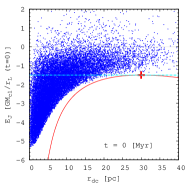
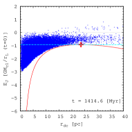
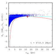
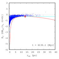
Figure 7: The $E_{\mathrm{J}}$ distribution of all bound stars as function of distance to the cluster centre $r_{\mathrm{dc}}$ defined by the density centre for different times of model 10. The full (red) lines are the same as in Figure 6. The dashed (cyan) lines mark the critical Jacobi energy.

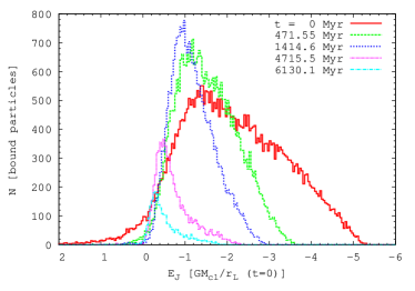
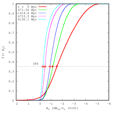
Figure 8: Top: The Jacobi energy distribution of bound particles at different times of model 10. Bottom: The cumulative distribution of bound particles as function of decreasing Jacobi energy for different times. The critical Jacobi energy is marked by crosses.

4.2 Tidal tail clumps

The structure of the tidal tails are determined by the angular momentum offset $\Delta L$ and energy excess $\Delta E$ of the stars. All stars move on epicycles with angular frequency $\kappa$. The epicentres are determined by $\Delta L$ (see equation 20) and the amplitudes by $\Delta E$ (see equation 2.3). Clumps form at the pericentres, where the streaming velocity is minimal. Figure 9 shows the clumps in the tidal tails for two different times. The local density at the position of each star is determined by the neighbour criterion of Casertano & Hut (1985) using 10 neighbours. It is colour coded in logarithmic scale. Note that the clump density does not decrease with decreasing cluster mass. The circle marks the tidal radius. The structure is similar in the trailing and leading arm as expected from the symmetry in the epicyclic approximation.

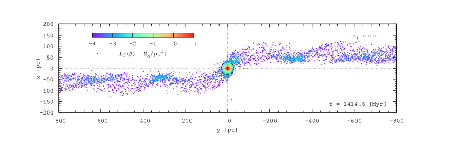
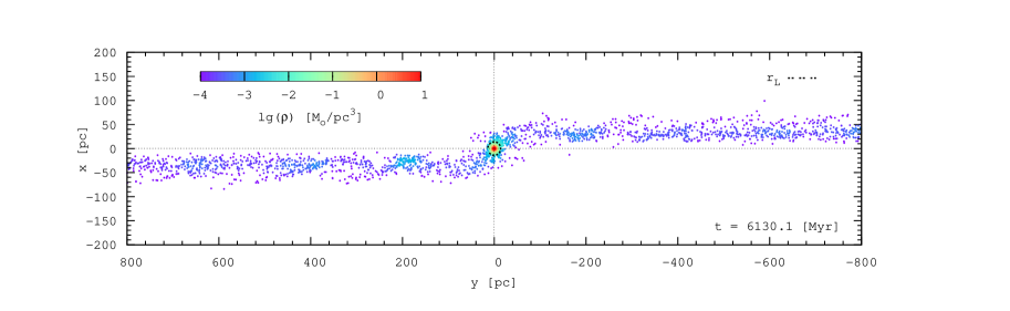
Figure 9: Positions and local densities of the stars of model 10 at an early and late time with about 50% and 10% bound mass, respectively.

The radial offset $\Delta R_{0}$ of the epicentres of the tidal tail stars is predicted by equation 20 from the measured $\Delta L$. In Figure 10 the histograms of calculated $\Delta R_{0}$ scaled to the corresponding tidal radii $r_{\mathrm{L}}$ are shown for different times. For the time resolution we have selected stars at tangential distances 200 pc$<|y|<$400 pc. We find that $\Delta R_{0}$ is proportional to $r_{\mathrm{L}}$ which scales with $M_{\mathrm{cl}}^{1/3}$. In the next section we quantify the scaling. The corresponding distributions of Jacobi energies $E_{\mathrm{J}}$ are shown in the lower panel of Figure 10. Here $E_{\mathrm{J}}$ is normalized to the actual $GM_{\mathrm{cl}}(t)/r_{\mathrm{L}}(t)$.

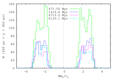
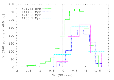
Figure 10: Top: The histograms show the distribution of the radial offsets $N(\Delta R_{0})$ of model 10 at different evolution times normalized to the corresponding tidal radii $r_{\mathrm{L}}(t)$. Stars at distances between 200 pc$<|y|<$400 pc along the tidal arms were selected. Bottom: The Jacobi energy distribution $N(E_{\mathrm{J}})$ of the same stars normalized to the actual $GM_{\mathrm{cl}}(t)/r_{\mathrm{L}}(t)$. Note that $N$ is the number of particles per bin and the bin width varies due to the different scaling.

The tangential positions of the clumps are multiples of $y_{0}(T)$, which are connected to $\Delta L$ (equation 2.3). Figures 11 and 12 show a comparison of the density distribution along the tidal tails and predicted histograms of $1,2,3\times y_{0}(T)$ for the early and late time. The position and width of the clumps agree well in both plots and the second and third clump show some overlap as predicted.

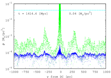
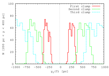
Figure 11: Density and $y_{0}(T)$ plot along the tidal tails at t=1.4 Gyr of model 10. Grey (green) dots are the local densities and black (blue) dots show the mean density averaged over a 30 pc sphere. The horizontal line corresponds to the stellar density in the solar neighbourhood.

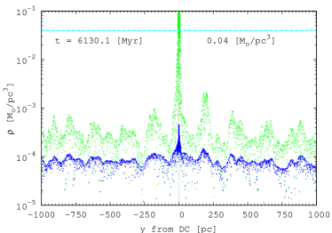
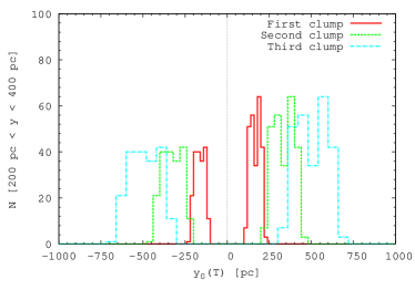
Figure 12: Same as in Figure 11 at time t=6.1 Gyr.

A similar comparison of the apo- and pericentre distribution in the radial coordinate of the numerical simulation also matches the spread of the analytic prediction.

In Figure 13 the peri- and apocentre positions of the selected stars are shown as function of $\Delta R_{0}$. There is a strong correlation between epicentre offset $\Delta R_{0}$ and amplitude, that is of $\Delta L$ and $\Delta E$. The double dotted (black) line shows the epicentre position and the dotted (blue) lines show the pericentre position with $v_{\mathrm{t}}=0$ and the corresponding apocentre (cycloids in the corotating reference frame). The dot-dashed (orange) lines are for $E_{\mathrm{J}}=0$ which determines the maximum amplitude for most stars. Only very few stars fall outside this limit. The orbit adopted by Küpper et al. (2008) with ($x,v$)=($r_{\mathrm{L}},0$) is marked by the (blue) crosses. It is a typical orbit with a slightly smaller epicentre offset $\Delta R_{0}$ compared to the mean value. Therefore they underestimated the distance of the clumps slightly as was already obvious from their simple $N$-body simulation.

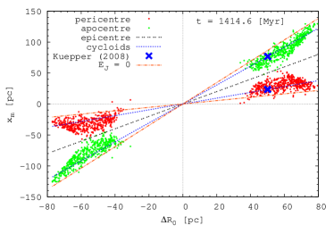
Figure 13: Apo- and pericentre positions of tidal tail stars of model 10 as function of $\Delta R_{0}$. The double-dotted (black) line shows the epicentre position, the dotted (blue) lines are the peri- and apocentre positions with zero velocity at pericentre in the corotating frame, and the dot-dashed (orange) lines are peri- and apocentre positions with $E_{\mathrm{J}}=0$. The cross marks the orbital parameters adopted in Küpper et al. (2008).

4.3 Parameter variation

In models 01-09 of Table 2 we vary the cluster mass and the galactocentric distance. Model 10 at an exact circular orbit differs in the evolution of model 08 only in a small modulation of the mass loss. Therefore we discuss here models 01-09 only. In the Section 4.4 a model near the galactic centre is discussed to show that the theory holds also in this extreme case.

Already in the temporal evolution of model 10 we found that the tidal tail structure scales with the tidal radius $r_{\mathrm{L}}$. For testing the dependence of $\Delta R_{0}$ and $y_{0}(T)$ on the cluster mass $M_{\mathrm{cl}}$ and on the distance $R_{\mathrm{C}}$ to the Galactic centre we measure for all nine models the value of $y_{0}(T)$ numerically. We add the trailing and leading arm density distributions and determine $y_{0}(T)$ by fitting the positions of clumps 1 and 2 to the value of 1$\times y_{0}(T)$ and 2$\times y_{0}(T)$. The result is plotted in Figure 14. The upper panel shows the mass dependence. Best power law fits for each $R_{\mathrm{C}}$ give a power law index of 1/3 to better than 1%. We test the scaling of $\Delta R_{0}$ with $r_{\mathrm{L}}$ by defining a scaling factor $A$

$$\Delta R_{0}=A\,r_{\mathrm{L}}$$ (34)

and calculating $A$ from $y_{0}(T)$ using equation 21

$$A=\frac{1}{\pi}\frac{\beta}{4-\beta^{2}}\frac{y_{0}(T)}{r_{\mathrm{L}}}$$ (35)

The result for the nine models is shown in the lower panel of Figure 14. The values of $A$ are independent of $y_{0}(T)$, that is of $M_{\mathrm{cl}}$ and $R_{\mathrm{C}}$. The best fit value is $A=2.77\pm 0.02$. A possible dependence on $\beta$ cannot be tested here, because the $\beta$ values are very similar. A further discussion is given in Section 4.4.

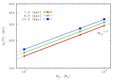
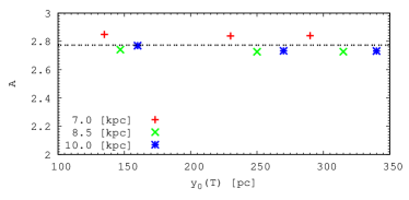
Figure 14: Top: Mass dependence of $y_{0}(T)$ for the nine different models. The lines show power law best fits of $y_{0}$. The points and lines are sampled by galactocentric distance. Bottom: Scaling factor $A=\Delta R_{0}/r_{\mathrm{L}}$ for models 01-09 with the same coding as above and the best fit value for $A$.

4.4 The Galactic centre case

Table 3: The list of tidal clump parameters for the Galactic centre case as described in the text.

Arm	Clump	$\Delta L/L_{\mathrm{C}}$	$\varphi_{0}$ [deg.]	$\varphi_{\mathrm{L1}}[deg.]$	$\varphi_{\mathrm{L2}}$ [deg.]	$\Delta\varphi/\varphi_{0}$ [%]	$r_{\mathrm{L}}$ [pc]	$y_{0}$ [pc]	$A_{\mathrm{\varphi}}$	$A_{\mathrm{L2}}$	$\Delta A/A_{\mathrm{L2}}$ [%]
Leading	1	-0.2179	51.6	43.3	44.1	14.5	2.45	16.9	1.81	1.54	14.9
	2	-0.2242	55.3	44.5	45.4	17.9	2.76	18.1	1.72	1.40	18.6
Trailing	1	0.2835	65.8	56.3	54.8	16.7	2.45	21.6	2.31	1.95	15.6

Near the Galactic centre the tidal forces are much stronger and the size of star clusters relative to the distance to the Galactic centre is much larger. Therefore it is an interesting case to test the epicyclic approximation in this extreme regime. We use the code nbody6gc to simulate the evolution of a star cluster in the tidal field of the Galactic centre. This code is based on the parallel $N$-body code nbody6++ (Aarseth, 1999, 2003; Spurzem, 1999) and in detail described in Ernst et al. (2008). The orbits of the stars in the star cluster are followed with a $4$th-order Hermite scheme (Makino & Aarseth, 1992) including Kustaanheimo-Stiefel regularization of close encounters (Kustaanheimo & Stiefel, 1965) and Chain regularization (Mikkola & Aarseth, 1998). In addition, the orbit of the star cluster in the analytic background potential of the galactic centre is followed using an $8$th-order composition scheme (Yoshida, 1990; McLachlan, 1995) including the Chandrasekhar dynamical friction force with a variable Coulomb logarithm (Just & Peñarrubia, 2005). The dissipative force is numerically implemented with an implicit midpoint method (Mikkola & Aarseth, 2002).

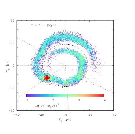
Figure 15: Clumps in the tidal tails of a star cluster with $N=10^{5}$ particles near the Galactic centre at $t=1.3$ Myr. The color coding shows the local stellar density in logarithmic scale. The solid lines show the tidal radius and assigns the galactocentric distance of the cluster. The radial lines mark the angles of the first and second clump of the leading arm and the first clump of the trailing arm with respect to the cluster centre.

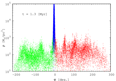
Figure 16: Density along the tidal arms as a function of the angle with respect to the cluster centre. The density maxima can be clearly identified. Stars inside the tidal radius corresponding to bound stars are in black (blue), the leading arm in dark grey at positive angles (red), and the trailing arm in light grey at negative angles (green). The wrap of the tidal tails can be seen from the $\varphi$-range exceeding 360⁰.

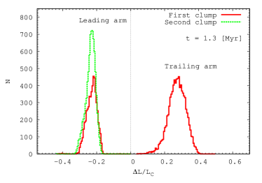
Figure 17: Histogram of angular momentum differences $\Delta L/L_{\mathrm{C}}$ scaled by the angular momentum of the circular orbit. $N$ is the number of particles with a certain angular momentum difference. Only stars within 25 degrees around the density maxima in the clumps have been included in the statistics.

For the Galactic centre, we used a scale free model (i.e., with a power law density profile, e.g. Mezger et al. (1996)) with a supermassive black hole (Eisenhauer et al., 2005) added at the centre. The cumulative mass profile is given by $M(R)=M_{\mathrm{bh}}+M_{0}(R/R_{0})^{\alpha}$. The parameters were taken to roughly match those in the centre of the Milky Way. We used $M_{\mathrm{bh}}=3.6\times 10^{6}M_{\odot}$, $M_{0}=1.67\times 10^{8}M_{\odot}$ at $R_{0}=20$ pc and $\alpha=1.2$. At a distance of $R_{\mathrm{C}}$=20 pc the influence of the central black hole can be neglected and the model is scale free. In the limit of a scale free model, the ratio $\beta=\kappa/\Omega$ is independent of galactocentric distance and is given by $\beta_{\mathrm{S}}^{2}=\alpha+1=2.2$. For the star cluster, we used a King model (King, 1966) with $W_{0}=6$, mass of $M_{\rm cl}=10^{6}M_{\odot}$, and half-mass radius of $r_{\mathrm{h}}=1.64$ pc starting at a galactocentric radius of $R_{\mathrm{C}}=20$ pc. The particle number is $N=10^{5}$. The initial tidal radius is $r_{\mathrm{L}}=2.72$ pc (mean of L1 and L2).

Figure 15 shows the tidal arms for the simulation after an evolution time of $t$=1.3 Myr. At $t$=1.3 Myr the galactocentric distance has slowly decayed due to dynamical friction to $R_{\mathrm{C}}=18.8$ pc and the tidal radius decayed mainly due to cluster mass loss to $r_{\mathrm{L}}=2.26$ pc according to equation 13 (both marked by circles). The local density is colour coded showing clearly the density maxima in the tidal tails. Three clumps can be identified in the leading arm and two clumps in the trailing arm. The radial lines from the Galactic centre mark the angles of three of these clumps with respect to the cluster centre.

Figure 16 shows the density along the tidal arms as a function of azimuth angle $\varphi$ with respect to the cluster centre. The clumps can be clearly identified as peaks. The $\varphi$-range exceeds 360⁰ showing the wrap of the tidal tails.

Figure 17 shows the histogram of the number of stars as function of angular momentum difference $\Delta L/L_{\mathrm{C}}$. We included only stars within an angle of 25 degrees around the density maxima in the statistics. The distribution is asymmetric with respect to the leading and trailing arms which cannot be explained in the frame of the epicyclic theory. The maxima in the histogram correspond to the density maxima of the clumps in the leading and trailing arms, respectively.

The measured angles $\varphi_{0}=y_{0}(T)/R_{\mathrm{C}}$ of the density maxima in the clumps can be compared to the theoretical estimates $\varphi_{\mathrm{L}}$ detrived from $\Delta L$. Note that these are the angles between the cluster centre and the first clump or the first and the second clump. For the theoretical estimate, we plugged the most frequent angular momentum differences of the leading and trailing arms from Figure 17 into equation

$$\varphi = \frac{2\pi}{\beta_{\mathrm{S}}}\left[1-\frac{\Omega_{\mathrm{C}}}{\Omega}\right]$$ (36)

$$\simeq \frac{2\pi}{\beta_{\mathrm{S}}}\left[\frac{\beta_{\mathrm{S}}^{2}-4}{\beta_{\mathrm{S}}^{2}}\frac{\Delta L}{L_{\mathrm{C}}}-\frac{\beta_{\mathrm{S}}^{2}-2}{\beta_{\mathrm{S}}^{2}}\frac{\beta_{\mathrm{S}}^{2}-4}{\beta_{\mathrm{S}}^{2}}\frac{\Delta L^{2}}{L_{\mathrm{C}}^{2}}\right].$$ (37)

Compared to equation 2.3 we added here the second order term to test the sensitivity of the results. The results are shown in Table 3 for the first two clumps in the leading arm and the first clump in the trailing arm. The density maximum of the second clump in the trailing arm is not well-defined. We denoted the measured angle as $\varphi_{0}$. The theoretical estimates from the measured $\Delta L/L_{\mathrm{C}}$ have been denoted as $\varphi_{\mathrm{L1}}$ (first-order) and $\varphi_{\mathrm{L2}}$ (second-order). We defined $\Delta\varphi=\varphi_{0}-\varphi_{\mathrm{L2}}$ for the error. Note that $\varphi_{\mathrm{L2}}$ is systematically lower than $\varphi_{0}$, but in principle we find a good agreement between measurement and theory. We also calculate the A values $A_{\mathrm{L2}}$ and $A_{\mathrm{\varphi}}$ from equations (34) and (35). $A_{\mathrm{L2}}$ is calculated from the Taylor expansion of $\Delta R_{0}$ in $L$ to second-order. For $A_{\mathrm{\varphi}}$ we used the measured $y_{0}=R_{\mathrm{C}}\varphi_{0}$. We used the tidal radius according to equation (13) at the time $t-cT$, where the stars in the clumps were released from the cluster. Here $T$ is the epicyclic period at $R_{\mathrm{C}}$ and $c=1$ and $c=2$ correspond to the first and second clump, respectively. We defined $\Delta A=A_{\mathrm{\varphi}}-A_{\mathrm{L2}}$ for the error. Again, the agreement is relatively good. However, the $A$ value is significantly smaller than that at large galactocentric distances.

There are some aspects of the tidal tail structure which cannot be explained by the simple epicyclic theory. The most prominent one is the asymmetry in the tidal arms concerning the angular momentum and Jacobi energy distribution. The errors $\Delta\varphi/\varphi_{0}$ and $\Delta A/A_{L2}$ stem from a slight non-conservation of angular momentum in the tidal arms. The reason is the influence of the cluster potential. This needs to be investigated further. The asymmetry between the inner and outer Lagrange points with respect to the central potential of the cluster is only a few percent. However, due to the proximity to the Galactic centre, the phase space for the particles which escape into the leading arm is considerably smaller than for those which escape into the trailing arm. The streaming velocitiy differs considerably between the leading and trailing arms. Thus the redistribution of energy and angular momentum for fixed $E_{\mathrm{J}}$ can be different. Since the radial offset is not small compared to the distance to the Galactic centre, an epicyclic theory for larger amplitudes would be helpful. A Taylor expansion in $\eta=1/R$ holds up to eccentricities of 0.5 as was shown by Dekker (1976) (see also Arifyanto & Fuchs (2006) for a derivation in the solar neighbourhood). For a further investigation we refer to Ernst et al. (2008), where the effects due to third- and higher-order terms in the Taylor expansion of the effective potential are discussed.

5 Summary

We presented a quantitative derivation of the angular momentum and energy distribution of escaping stars from a star cluster in the tidal field of the Milky Way. Despite the motion on a circular orbit, the tidal tails are clumpy due to the epicyclic motion of the stars. We compared the derived distances and widths of the clumps with numerical simulations using star-by-star simulations. For star clusters at the solar circle we included an IMF and mass loss due to stellar evolution in the calculations. The same equations were applied to a star cluster very close to the Galactic centre, where the tidal forces are very strong.

We find a very good agreement of theory and models concerning the tidal tail structure. The positions of the clumps are determined by the angular momentum offset of the stars, which lead to a radial offset of the epicenters with respect to the cluster orbit. The investigation of Küpper et al. (2008) is a special case of our investigations but for a Kepler potential. We find that the radial offset of the tidal arms is proportional to the tidal radius. However near the Galactic centre the factor of proportionality is considerably smaller.

The tidal arm structure at large galactocentric radii is symmetric, whereas the asymmetry near the galactic centre is considerable. This can be reproduced only partly by taking into account the correction of the epicyclic frequency at the epicentre radii.

We have also measured the Jacobi energy distribution of bound stars and showed that there are 35% of stars above the critical Jacobi energy independent of the evolutionary state of the cluster. These stars can potentially leave the cluster. This is a hint, that mass loss is dominated by a self-regulating process of increasing Jacobi energy due to the diminishing gravitational potential of the star cluster induced by the mass loss itself.

Finally we consider the observability of the predicted clump properties in the tidal tails of star clusters. The identification of tidal tail stars of open clusters on a circular orbit is strongly hampered by the large number of nearby field stars with similar properties. But with differential methods using high quality data for distances and velocities it may be possible to identify the most prominent first clumps. We have shown that the maximum density in the first clump does not decrease with time until dissolution of the cluster. The first clumps are formed by escaping stars with a time delay determined by the epicyclic period $T_{\kappa}\approx 150$ Myr. The tidal tail structure will probably survive the gravitational scattering process, which is also responsible for the galactic disc heating (Wielen, 1977). On a timescale of one epicyclic period, we expect only small perturbations of the tidal clump position and velocity but no destruction. The density maximum of the first clump is of the order of a few percent of the field density of the galactic disc. The velocity imprint by the epicyclic motion is of the order of 2 km/s. An overdensity with these properties may be difficult to observe for clusters on exact circular orbits, if there is no additional separating property. For young star clusters the high fraction of early type stars can serve for such a discrimination. On the other hand most star clusters are identified by the systematic peculiar motion with respect to the field stars. If the positions and velocities of the tidal clump stars are properly predicted, they may be observable as moving groups.

For an application of the tidal clump theory to the eccentric orbits of globular clusters a perturbation theory with respect to the ’free falling’ comoving coordinate system would be necessary. In this case the Jacobi energy is no longer a constant of motion. This will be a matter of future investigations. Some numerical test runs have shown that tidal tail clumps are formed also on highly eccentric orbits without an additional external perturbation, but the geometry and density is modulated along the orbital position.

6 ACKNOWLEDGEMENTS

P. B. & M. P. thanks for the special support of his work by the Ukrainian National Academy of Sciences under the Main Astronomical Observatory GRAPE/GRID computing cluster project.

P. B. acknowledges his support from the German Science Foundation (DGF) under SFB 439 (sub-project B11) at the University of Heidelberg. His work was also supported by the Volkswagen Foundation GRACE Project No. I80 041-043.

M. P. acknowledges support by the University of Vienna through the frame of the Initiative Kolleg (IK) ”The Cosmic Matter Circuit” I033-N and computing time on the Grape Cluster of the University of Vienna.

A. E. would like to thank Rainer Spurzem, Ortwin Gerhard and Kap-Soo Oh for the provision of an earlier version of nbody6gc and gratefully acknowledges support by the International Max Planck Research School (IMPRS) for Astronomy and Cosmic Physics at the University of Heidelberg.

We thank the DEISA Consortium (www.deisa.eu), co-funded through EU FP6 projects RI-508830 and RI-031513, for support within the DEISA Extreme Computing Initiative and the Astrogrid-D, which links together the two GRAPE clusters in Kiev and Heidelberg.

Appendix A Taylor expansions

We use Taylor expansions of the radial variation of different quantities in the gravitational field of the Galaxy in $R$ and $L$ with respect to some circular orbit with $R_{0}$ and $L_{0}$. The potential $\Phi_{\mathrm{cl}}$ of the star cluster is not expanded. The Taylor expansions are applied to: 1) the energy of stars on eccentric orbits with fixed $L$ in the galactic field; 2) the effective potential in the cluster frame; 3) the epicentre position and energy excess of tidal tail stars in the cluster frame. For the Taylor expansions we use

$$\kappa^{2} = 2\Omega^{2}\left(2+\frac{\mbox{\rm d}\ln\Omega}{\mbox{\rm d}\ln R}\right)$$ (38)

$$\beta=\frac{\kappa}{\Omega} \mathrm{and} \beta^{\prime}=\frac{\mbox{\rm d}\beta}{\mbox{\rm d}\ln R}$$ (39)

$$\frac{\mbox{\rm d}\Phi_{\mathrm{g}}}{\mbox{\rm d}R}=\Omega^{2}R \mathrm{and} \frac{\mbox{\rm d}\ln\Omega}{\mbox{\rm d}\ln R}=\frac{\beta^{2}-4}{2}$$ (40)

with angular speed $\Omega$ and epicyclic frequency $\kappa$.

For the epicyclic motion in the tidal tails (Sec. 2.1 and 4.4) the gravitational potential of the galaxy is needed in terms of $r=R-R_{0}$. We find to third order

$$\Phi_{\mathrm{g}}(R) = \Phi_{\mathrm{g}}(R_{0})+\frac{L_{0}^{2}}{R_{0}^{3}}r+\left(\beta_{0}^{2}-3\right)\frac{L_{0}^{2}}{R_{0}^{4}}\frac{r^{2}}{2}$$ (42)

$$+\left[(\beta_{0}^{2}-3)(\beta_{0}^{2}-4)+2\beta_{0}\beta^{\prime}_{0}\right]\frac{L_{0}^{2}}{R_{0}^{5}}\frac{r^{3}}{6}$$

For the apo- and pericentre $R_{\mathrm{m}}=R_{0}+r_{\mathrm{m}}$ we find for the kinetic energy

$$\frac{L_{0}^{2}}{2R_{\mathrm{m}}^{2}} = \frac{L_{0}^{2}}{2R_{0}^{2}}\left(1-2\frac{r_{\mathrm{m}}}{R_{0}}+3\frac{r_{\mathrm{m}}^{2}}{R_{0}^{2}}-4\frac{r_{\mathrm{m}}^{3}}{R_{0}^{3}}\right)$$ (43)

leading to the energy excess $\Delta E=E-E_{0}$ (relative to the circular orbit with the same angular momentum $L_{0}$)

$$\Delta E = \frac{\beta_{0}^{2}}{2}\frac{L_{0}^{2}}{R_{0}^{4}}r_{\mathrm{m}}^{2}+\left[\beta_{0}^{2}(\beta_{0}^{2}-7)+2\beta_{0}\beta^{\prime}_{0}\right]\frac{L_{0}^{2}}{R_{0}^{5}}\frac{r_{\mathrm{m}}^{3}}{6}$$ (44)

For the derivation in the rest frame of the star cluster we need the Taylor expansions of $R(L)$, $\Omega(L)$ and $\Phi_{\mathrm{g}}(L)$ with respect to $\Delta L=L-L_{\mathrm{C}}$ ($L$ is the angular momentum of the circular orbit at radius $R(L)$). In terms of position $x$ and velocity $v_{\mathrm{r}},v_{\mathrm{t}}$ in the corotating frame we have

$$\Delta L=(v_{\mathrm{t}}+\Omega_{\mathrm{C}}R)R-\Omega_{\mathrm{C}}R_{\mathrm{C}}^{2}=(2\Omega_{\mathrm{C}}x+v_{\mathrm{t}})R_{\mathrm{C}}+\Omega_{\mathrm{C}}x^{2}+v_{\mathrm{t}}x$$ (45)

The Taylor expansions in $L$ are

$$R(L) = R_{\mathrm{C}}+\frac{2}{\beta_{\mathrm{C}}^{2}}\frac{R_{\mathrm{C}}}{L_{\mathrm{C}}}\Delta L$$

$$+\frac{1}{\beta_{\mathrm{C}}^{4}}\left[(2-\beta_{\mathrm{C}}^{2})-\frac{4\beta^{\prime}}{\beta}\right]\frac{R_{\mathrm{C}}}{L_{\mathrm{C}}^{2}}\Delta L^{2}$$

$$\Phi_{\mathrm{g}}(L) = \Phi_{g,C}+\frac{2}{\beta_{\mathrm{C}}^{2}}\Omega_{\mathrm{C}}\Delta L$$

$$+\frac{1}{\beta_{\mathrm{C}}^{4}}\left(\beta_{\mathrm{C}}^{2}-4-2\frac{\beta^{\prime}_{\mathrm{C}}}{\beta_{\mathrm{C}}}\right)\Omega_{\mathrm{C}}\frac{\Delta L^{2}}{L_{\mathrm{C}}}$$

$$\frac{\Omega(L)L}{2} = \frac{\Omega_{\mathrm{C}}L_{\mathrm{C}}}{2}+\frac{\beta_{\mathrm{C}}^{2}-2}{\beta_{\mathrm{C}}^{2}}\Omega_{\mathrm{C}}\Delta L$$

$$+\frac{1}{2\beta_{\mathrm{C}}^{4}}\left((\beta_{\mathrm{C}}^{2}-2)(\beta_{\mathrm{C}}^{2}-4)+4\frac{\beta^{\prime}_{\mathrm{C}}}{\beta_{\mathrm{C}}}\right)\Omega_{\mathrm{C}}\frac{\Delta L^{2}}{L_{\mathrm{C}}}$$

$$\frac{1}{\Omega(L)} = \frac{1}{\Omega_{\mathrm{C}}}-\frac{\beta_{\mathrm{C}}^{2}-4}{\beta_{\mathrm{C}}^{2}}\frac{1}{\Omega_{\mathrm{C}}}\frac{\Delta L}{L_{\mathrm{C}}}$$

$$+\frac{1}{\beta_{\mathrm{C}}^{4}}\left((\beta_{\mathrm{C}}^{2}-2)(\beta_{\mathrm{C}}^{2}-4)-8\frac{\beta_{\mathrm{C}}^{\prime}}{\beta_{\mathrm{C}}}\right)\frac{1}{\Omega_{\mathrm{C}}}\frac{\Delta L^{2}}{L_{\mathrm{C}}^{2}}$$

Here already second order terms contain $\beta^{\prime}$. Since $\beta\beta^{\prime}=\mbox{\rm d}^{2}\ln\Omega/\mbox{\rm d}(\ln R)^{2}$, the logarithmic derivative $\beta^{\prime}$ vanishes only, if $\Omega(R)\propto R^{\alpha}$ is exactly a power law with constant $\alpha$. For realistic rotation curves $\beta$ varies considerably (see Fig. 3). We find the energy excess $\Delta E_{0}=E_{0}-E_{\mathrm{C}}$ of the epicentre motion for equation 23 by adding equations A and A

$$\Delta E_{0} = \Omega_{\mathrm{C}}\Delta L+\frac{1}{2\beta_{\mathrm{C}}^{2}}\left(\beta_{\mathrm{C}}^{2}-4\right)\Omega_{\mathrm{C}}\frac{\Delta L^{2}}{L_{\mathrm{C}}}$$ (50)

Here the $\beta^{\prime}$ term vanishes.

For the derivation in the rest frame of the star cluster we need $\Phi_{\mathrm{eff}}$ only in terms of $r=R-R_{\mathrm{C}}$. The cluster potential is not expanded in a Taylor series. We find

$$\Phi_{\mathrm{eff}}(R) = \Phi_{\mathrm{cl}}+\Phi_{\mathrm{g,eff}}(R_{\mathrm{C}})+\frac{\beta_{\mathrm{C}}^{2}-4}{2}\Omega_{\mathrm{C}}^{2}r^{2}+$$ (51)

$$\left[(\beta_{\mathrm{C}}^{2}-3)(\beta_{\mathrm{C}}^{2}-4)+2\beta_{\mathrm{C}}\beta^{\prime}_{\mathrm{C}}\right]\Omega_{\mathrm{C}}^{2}\frac{r^{3}}{6R_{\mathrm{C}}}$$

References

- Aarseth et al. (1974) Aarseth S.J., Hénon M., Wielen R., 1974, A&A, 37, 183
- Aarseth (1999) Aarseth S. J., 1999, PASP, 111, 1333
- Aarseth (2003) Aarseth S. J., 2003, Gravitational -body Simulations - Tools and Algorithms, Cambridge Univ. Press
- Arifyanto & Fuchs (2006) Arifyanto M.I., Fuchs B., 2006, A&A, 449, 533
- Berczik et al. (2005) Berczik P., Merritt D., Spurzem R., 2005, ApJ, 633, 680
- Berczik et al. (2006) Berczik P., Merritt D., Spurzem R., Bischof H.-P., 2006, ApJL, 642, L21
- Binney & Tremaine (1987) Binney J., Tremaine S., 1987, Galactic dynamics, Princeton univ. press, New Jersey
- Capuzzo Dolcetta et al. (2005) Capuzzo Dolcetta R., Di Matteo P., Miocchi P., 2005, AJ, 129, 1906
- Casertano & Hut (1985) Casertano S., Hut P., 1985, ApJ, 298, 80
- Dekker (1976) Dekker E., 1976, Phys Rep., 24, 315
- Douphole & Colin (1995) Douphole B. & Colin J., 1995, A&A, 300, 117
- Eisenhauer et al. (2005) Eisenhauer F., Genzel R., Alexander T., et al., 2005, ApJ, 628, 246
- Ernst et al. (2008) Ernst A., Just A., Spurzem R., 2008, On the dissolution of star clusters in galactic centres. I. Circular orbits., 2008, MNRAS, subm.
- Fukushige et al. (2000) Fukushige T., Heggie D.C., 2000, MNRAS, 318, 753
- Harfst et al. (2007) Harfst S., Gualandris A., Merritt D., Spurzem R., Portegies Zwart S., Berczik P., 2007, NewA, 12, 357
- Inoue & Kamaya (2000) Inoue A.K. & Kamaya H., 2000, PASJ, 52, L47
- Just & Peñarrubia (2005) Just, A., Penarrubia J., 2005, A&A, 431, 861
- Kharchenko et al. (2008) Kharchenko N.V., Berczik P., Petrov M.I., Piskunov A.E., Röser S., Schilbach E., Scholz R.-D., 2008, A&A, subm.
- King (1966) King I. R., 1966, AJ, 71, 64
- Kustaanheimo & Stiefel (1965) Kustaanheimo P. & Stiefel E., 1965, J. Reine Angew. Math., 218, 204
- Küpper et al. (2008) Küpper A.H.W., Macleod A., Heggie D.C., 2008, MNRAS, 387, 1248
- Larson (1981) Larson R.B., 1981, MNRAS, 194, 809
- Leon et al. (2000) Leon S., Meylan G., Combes F., 2000, A&A, 359, 907
- Makino & Aarseth (1992) Makino J. & Aarseth S. J., 1992, PASJ, 44, 141
- Maloney (1990) Maloney P., 1990, ApJ, 349, L9
- McLachlan (1995) McLachlan R., 1995, SIAM J. Sci. Comp. 16, 151
- Merritt et al. (2007) Merritt D., Berczik P., Laun F., 2007, AJ, 133, 553
- Mezger et al. (1996) Mezger P. G., Duschl W. J., Zylka R., 1996, A&A Rev., 7, 289
- Mikkola & Aarseth (1998) Mikkola S. & Aarseth S.J., 1998, NewA, 3, 309
- Mikkola & Aarseth (2002) Mikkola S. & Aarseth S.J., 2002, Cel. Mech. Dyn. Astron., 84, 343
- Miyamoto & Nagai (1975) Miyamoto M. & Nagai R., 1975, PASJ, 27, 533
- Odenkirchen et al. (2001) Odenkirchen M., Grebel E.K., Rockosi C.M. et al., 2001, ApJL, 548, L165
- Odenkirchen et al. (2003) Odenkirchen M., Grebel E.K., Dehnen W. et al., 2003, AJ, 126, 2385
- Raiteri et al. (1996) Raiteri C.M., Villata M., Navarro J.F., 1996, A&A, 315, 105
- Salpeter (1955) Salpeter E.E., 1955, ApJ, 121, 161
- Solomon et al. (1987) Solomon P.M., Rivolo A.R., Barrett J., Yahil A., 1987, ApJ, 319, 730
- Spurzem (1999) Spurzem R., 1999, J. Comp. Appl. Math., 109, 407
- Theis & Hensler (1993) Theis Ch. & Hensler G., 1993, A&A, 280, 85
- van den Hoek & Groenewegen (1997) van den Hoek L.B. & Groenewegen M.A.T., 1997, A&AS, 123, 305
- Wielen (1977) Wielen R., 1977, A&A, 60, 263
- Yoshida (1990) Yoshida H., 1990, Phys. Lett. A, 150, 262