Effects of an oscillating field on magnetic domain patterns: Emergence of concentric-ring patterns surrounding a strong defect

Abstract

Oscillating fields can make domain patterns change into various types of structures. Numerical simulations show that concentric-ring domain patterns centered at a strong defect are observed under a rapidly oscillating field in some cases. The concentric-ring pattern appears near the threshold of spatially-uniform patterns in high-frequency cases. The threshold is theoretically estimated and the theoretical threshold is in good agreement with numerical one in a high-frequency region. The theoretical analysis gives also good estimations of several characteristics of domain patterns for high-frequencies.

I Introduction

Rapidly oscillating fields cause interesting phenomena in a wide variety of systems. Those phenomena are often discussed in the view of stabilization of an unstable state. One of the simplest examples is the problem of Kapitza’s inverted pendulum, which was generalized by Landau and Lifshitz landau . The key idea is to separate the dynamics into a rapidly oscillating part and a slowly varying part. The method has been applied to various systems, e.g., the classical and quantum dynamics in periodically driven systems rahav03 ; rahav05 , the stabilization of a matter-wave soliton in two-dimensional Bose-Einstein condensates without an external trap saito ; abdullaev ; liu , and magnetic domain patterns traveling at a slow velocity under a rapidly oscillating field travel .

Domain patterns are observed in a wide variety of systems, and they show many kinds of structures (see, for example, Refs. cross ; seul ; muratov and references therein). Magnetic domain patterns are one of their good examples. While they usually exhibit a labyrinth structure under zero field, they also show other kinds of structures under an oscillating field. For instance, parallel-stripe and several kinds of lattice structures are observed in experiments and numerical simulations miura ; mino ; tsuka . Moreover, traveling patterns travel and more interesting patterns, e.g., spirals and concentric-ring patterns kandaurova ; mino_p , have been observed, depending on the strength and frequency of the field. Spirals and concentric-ring patterns appear under a large-amplitude and high-frequency field in experiments, and the field range where they appear is not wide.

In this paper, we investigate effects of an oscillating field by numerical simulations and theoretical analysis, focusing on the emergence of concentric-ring magnetic domain patterns surrounding a strong defect. Recently, two theoretical methods were proposed to investigate the effects of an oscillating field on pattern formation in ferromagnetic thin films travel . One gives the “time-averaged model” and the other gives the “phase-shifted model”: The former is derived by averaging out rapidly oscillating terms, and the latter includes the delay of the response to the oscillating field. In this paper, the time-averaged model is applied to theoretical analysis, since it is suitable for discussing “stationary” domain patterns which oscillate periodically but are unchanged in terms of a long-time average. The theoretical line of the threshold for nonuniform patterns is derived from the time-averaged model. The theoretical threshold is consistent with the numerically simulated one in a high-frequency region, where a concentric-ring pattern appears around the defect.

In fact, there are several techniques to study domain patterns under a rapidly oscillating field theoretically. Applying a multi-time-scale technique michaelis ; kirakosyan , one can obtain more complex equations in a better approximation than the time-averaged model. In other words, the time-averaged model corresponds to the lowest orders of multi-time-scale expansions. In this paper, the time-averaged model is employed since it has a simple form and is efficient enough to discuss the appearance of concentric-ring patterns in a high-frequency region.

The creation of a concentric-ring pattern can have different mechanisms. One of them is boundary conditions, and the strong defect is a kind of boundary condition. The selection of a pattern depends on boundary conditions as well as the field frequency or other parameters dong . For example, in nematic liquid crystals under a rotating magnetic field, it is sometimes observed that the center of concentric rings nucleated by a dust particle moves away from it migler ; Faraday experiments of viscous fluid and granular layers in round cells show concentric-ring patterns or spiral patterns kiyashko ; bruyn in some cases. On the other hand, concentric-ring patterns can also appear spontaneously. In fact, spiral patterns as well as concentric-ring patterns appear in the absence of a strong defect under some conditions kandaurova ; tuszynski . However, we will not consider spontaneously created concentric-ring patterns in this paper since those patterns are beyond the scope of this paper.

The rest of this paper is organized as follows. In Sec. II, the model of our system is introduced and numerical results, i.e., the phase diagram for concentric-ring patterns and profiles of the domain patterns, are exhibited. In Sec. III, we discuss the threshold for nonuniform patterns, employing the time-averaged model. Moreover, several characteristics of a domain pattern estimated from the time-averaged model are compared with those from the numerical simulations. The mechanism for the appearance of a concentric-ring pattern is discussed in Sec. IV. Conclusions are given in Sec. V.

II Numerical simulation

Our model is a simple two-dimensional model (see Refs. travel ; jagla04 ; kudo , and references therein). The Hamiltonian of the model consists of four energy terms: Uniaxial anisotropy energy $H_{\rm ani}$, exchange interactions $H_{J}$, dipolar interactions $H_{\rm di}$, and the interactions with the external field $H_{\rm ex}$. We consider a scalar field $\phi(\bm{r})$, where $\bm{r}=(x,y)$. The anisotropy energy is given by

$$H_{\rm ani}=\alpha\int{\rm d}\bm{r}\lambda(\bm{r})\left(-\frac{\phi(\bm{r})^{2}}{2}+\frac{\phi(\bm{r})^{4}}{4}\right),$$ (1)

where $\lambda(\bm{r})$ is employed to express the effect of defects or the roughness of a sample. This term implies that the values $\phi(\bm{r})=\pm 1$ are preferable. The positive and negative values of $\phi(\bm{r})$ correspond to up and down spins, respectively. The exchange and dipolar interactions are described by

$$H_{J}=\beta\int{\rm d}\bm{r}\frac{|\nabla\phi(\bm{r})|^{2}}{2}$$ (2)

and

$$H_{\rm di}=\gamma\int{\rm d}\bm{r}{\rm d}\bm{r}^{\prime}\phi(\bm{r})\phi(\bm{r}^{\prime})G(\bm{r},\bm{r}^{\prime}),$$ (3)

respectively. Here, $G(\bm{r},\bm{r}^{\prime})\sim|\bm{r}-\bm{r}^{\prime}|^{-3}$ at long distances. These two terms are competing interactions: $H_{J}$ implies that $\phi(\bm{r})$ tends to have the same value as neighbors, while $H_{\rm di}$ implies that $\phi(\bm{r})$ prefers to have the opposite sign to ones at some distances. The interactions with the external field is given by

$$H_{\rm ex}=-h(t)\int{\rm d}\bm{r}\phi(\bm{r}).$$ (4)

Here, we consider a spatially homogeneous and rapidly oscillating field,

$$h(t)=h_{0}\sin\omega t.$$ (5)

From Eqs. (1)–(4), the dynamical equation of the model is described by

$$\frac{\partial\phi(\bm{r})}{\partial t} = -\frac{\delta(H_{\rm ani}+H_{J}+H_{\rm di}+{H_{\rm ex}})}{\delta\phi(\bm{r})}$$ (6)

$$= \alpha\lambda(\bm{r})[\phi(\bm{r})-\phi(\bm{r})^{3}]+\beta\nabla^{2}\phi(\bm{r})-\gamma\int{\rm d}\bm{r}^{\prime}\phi(\bm{r}^{\prime})G(\bm{r},\bm{r}^{\prime})+h(t).$$

The numerical procedures are almost the same as those of Refs. travel ; jagla04 ; kudo . For time evolution, a semi-implicit method is employed: The exact solutions and the second-order Runge-Kutta method are used for the linear and nonlinear terms, respectively. For a better spatial resolution, a pseudo-spectral method is applied. Namely, the time evolutions are calculated for the equation in Fourier space corresponding to Eq. (6),

$$\frac{\partial\phi_{\bm{k}}}{\partial t}=\alpha[(\phi-\phi^{3})\lambda]_{\bm{k}}-(\beta k^{2}+\gamma G_{\bm{k}})\phi_{\bm{k}}+h(t)\delta_{\bm{k}},$$ (7)

where $[\cdot]$ denotes the convolution sum and $G_{\bm{k}}$ is the Fourier transform of $G({\bm{r}},0)$. Here, we define $G(\bm{r},0)\equiv 1/|\bm{r}|^{3}$. Then, one has

$$G_{\bm{k}}=a_{0}-a_{1}k,$$ (8)

where $k=|\bm{k}|$ and

$$a_{0}=2\pi\int_{d}^{\infty}\frac{{\rm d}r}{r^{2}},\quad a_{1}=2\pi.$$ (9)

Here, $d$ is the cutoff length of the dipolar interactions. In the simulations, we set $d=\pi/2$, which results in $a_{0}=4$.

The effect of a strong defect is incorporated in the anisotropy term, Eq. (1). Here, we put the strong defect at the center, i.e., the origin ($\bm{r}=\bm{0}$), as follows:

$$\lambda(\bm{r})=\left\{\begin{array}[]{rl}10&(\bm{r}=\bm{0}).\\ 1&(\bm{r}\neq\bm{0}).\end{array}\right.$$ (10)

This condition implies that the spin at the center will not flip unless the applied field is too strong. The parameters in Eqs. (1)–(3) are given as $\alpha=2$, $\beta=2$, and $\gamma=2\beta/a_{1}=2/\pi$. The simulations are performed on a $128\times 128$ lattice with periodic boundary conditions.

The concentric-ring patterns simulated by the numerical calculations appear in a limited region of the frequency ($\omega$) and the amplitude ($h_{0}$) of the external field. Figure 1 shows the $\omega$-$h_{0}$ phase diagram for concentric-ring patterns. The solid lines and the dashed line are drawn by using the results of the numerical simulations and theoretical analysis, respectively. The theoretical analysis is explained in Sec. III. Concentric-ring patterns are seen only in the region between the upper and lower solid lines. Above the upper solid line, one sees only spatially-homogeneous patterns except for the vicinity of the center. On the contrary, stripes, labyrinth or lattice structures appear below the lower solid line.

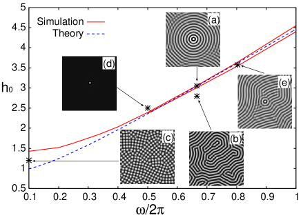
Figure 1: (Color online) Phase diagram for the concentric-ring patterns surrounding a strong defect at the center. The horizontal and vertical axes are the frequency ($\omega$) and the amplitude ($h_{0}$) of the external field, respectively. The red solid lines and blue dashed line are obtained from the numerical simulations and theoretical analysis, respectively. The values of $\omega$ and $h_{0}$ of each snapshot are as follows: (a) $\omega/2\pi=2/3\simeq 0.667$ and $h_{0}=3.05$, (b) $\omega/2\pi=2/3$ and $h_{0}=2.8$, (c) $\omega/2\pi=0.1$ and $h_{0}=1.2$, (d) $\omega/2\pi=0.5$ and $h_{0}=2.5$, and (e) $\omega/2\pi=0.8$ and $h_{0}=3.56$.

Actually, it is difficult to find the exact boundaries of the region where concentric-ring patterns appear. One may think that concentric-ring patterns can appear right on the numerical threshold line in a low-frequency region. However, even if a concentric-ring pattern could appear on the threshold, it would be hard to find its exact value. In a low-frequency region, the boundary between spatially-homogeneous patterns and nonuniform patterns (e.g., stripes, labyrinth, and lattice structures) is sharp. In contrast, in a high-frequency region, the boundaries between concentric-ring patterns and other patterns are unclear: They are crossover lines rather than transition ones. Actually, for high frequencies, a few concentric rings around the strong defect coexist with other patterns (i.e., stripes, labyrinth or lattice patterns) in the region near the boundary lines of the concentric-ring-pattern region. In other words, a few concentric rings start to appear at the lower boundary, and the number of rings grows as $h_{0}$ increases. At the upper boundary, nonuniform patterns disappear except for the vicinity of the strong defect.

The profile of each domain pattern is useful to see the time dependence of the pattern. The profiles corresponding to the snapshots (a) and (b) in Fig. 1 are shown in Fig. 2. The profile is a section which includes the center (the defect) and is perpendicular to $x$ axis (the horizontal axis). The profiles show that the pattern is oscillating without deformation except for the vicinity of the center. The amplitudes of the oscillation and that of the pattern (i.e., the difference between the maximum and minimum values of $\phi(\bm{r})$ except for the vicinity of the defect at a certain time) depend on the amplitude and frequency of the field.

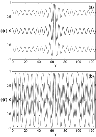
Figure 2: Profiles of the domain patterns corresponding to the snapshots (a) and (b) in Fig. 1: (a) $\omega/2\pi=2/3\simeq 0.667$ and $h_{0}=3.05$, (b) $\omega/2\pi=2/3$ and $h_{0}=2.8$. The upper and lower thin curves in each figure are the profiles at $t=(n+1/2)T$ and $t=nT$, respectively, where $n$ is an integer and $T=2\pi/\omega$. The middle thick curve is the time-averaged profile.

III Theoretical analysis

Since a rapidly oscillating field is applied, Kapitza’s idea landau is applicable to the analysis of the pattern formation in this system. In fact, the profiles in Fig. 2 validate the use of the idea. In other words, the results in Fig. 2 justify the fact that the variable $\phi(\bm{r},t)$ in Eq. (6) consists of a spatially homogeneous oscillating term $\phi_{0}(t)$ and a slowly varying term $\Phi(\bm{r},t)$. In this section, the domain patterns in the absence of a defect are discussed by employing the time-averaged model travel . Namely, $\lambda(\bm{r})$ in Eq. (10) is replaced by unity, i.e., $\lambda(\bm{r})=1$.

First of all, let us consider the spatially homogeneous oscillating solution $\phi_{0}(t)$ of Eq. (6). Then, one has

$$\dot{\phi_{0}}=\alpha(\phi_{0}-\phi_{0}^{3})-\gamma\phi_{0}\int{\rm d}\bm{r}^{\prime}|\bm{r}^{\prime}|^{-3}+h(t).$$ (11)

Its solution can be approximately written as

$$\phi_{0}=\rho\sin(\omega t+\delta),$$ (12)

where $\delta$ is a phase shift which comes from the delay of the response to the field. Substituting Eq. (12) into Eq. (11) and omitting high-order harmonics (i.e., $\sin 3\omega t$), one can evaluate $\rho$ and $\delta$. The value of $\rho$ is obtained from the following equations travel :

$$\frac{9}{16}\alpha^{2}\rho^{6}-\frac{3}{2}\alpha\eta_{0}\rho^{4}+(\omega^{2}+\eta_{0}^{2})\rho^{2}=h_{0}^{2},$$ (13)

where $\eta_{0}=\alpha-\gamma a_{0}$.

Now, we consider the equation for the slowly varying variable $\Phi(\bm{r},t)$ which describes a spatially dependent pattern. Substituting $\phi(\bm{r},t)=\phi_{0}(t)+\Phi(\bm{r},t)$ into Eq. (6) and averaging out the rapid oscillation, one obtains the time-averaged model

$$\frac{\partial\Phi(\bm{r})}{\partial t}=\left(1-\frac{3}{2}\rho^{2}\right)\alpha\Phi(\bm{r})+\beta\nabla^{2}\Phi(\bm{r})-\gamma\int{\rm d}\bm{r}^{\prime}\frac{\Phi(\bm{r}^{\prime})}{|\bm{r}-\bm{r}^{\prime}|^{3}}-\alpha\Phi(\bm{r})^{3}.$$ (14)

The linear stability of Eq. (14) leads to the theoretical curve in Fig. 1 corresponding to the threshold for the existence of nonuniform patterns. Substituting $\Phi(\bm{r})=\sum_{\bm{k}}\exp(i\bm{k}\cdot\bm{r})\Phi_{\bm{k}}$ into Eq. (14), one has the linear part of the equation written as

$$\frac{\partial\Phi_{\bm{k}}}{\partial t}=\eta_{\bm{k}}\Phi_{\bm{k}}.$$ (15)

Here,

$$\eta_{\bm{k}}=\left(1-\frac{3}{2}\rho^{2}\right)\alpha-\beta(k-k_{0})^{2}+\beta k_{0}^{2}-\gamma a_{0},$$ (16)

where $k=|\bm{k}|$ and $k_{0}=a_{1}\gamma/(2\beta)$. Since $\eta_{\bm{k}}$ has the maximum value at $k=k_{0}$, the value of $\rho$ for $\eta_{k=k_{0}}=0$ gives the instability threshold $\rho_{c}$,

$$\rho_{c}=\left[\frac{2}{3\alpha}(\alpha+\beta k_{0}^{2}-\gamma a_{0})\right]^{1/2}.$$ (17)

When $\rho>\rho_{c}$, $\eta_{\bm{k}}$ is negative for all values of $\bm{k}$. In other words, the homogeneous pattern, i.e., $\Phi(\bm{r})=0$, is stable and no inhomogeneous pattern tends to appear for $\rho>\rho_{c}$. The threshold curve for nonuniform patterns in Fig. 1 (the dashed line) is given by Eq. (13) with $\rho=\rho_{c}$.

Now, let us discuss how a nonuniform pattern disappears near the threshold. Taking $\Phi(\bm{r},t)=A\cos k_{0}x$ which is one of the simplest stable patterns and substituting it into Eq.(14), we have

$$\left[\left(1-\frac{3}{2}\rho^{2}\right)\alpha+\beta k_{0}^{2}-\gamma a_{0}-\frac{3}{4}\alpha A^{2}\right]A\cos k_{0}x-\frac{\alpha}{4}A^{3}\cos 3k_{0}x=0.$$ (18)

Neglecting the higher harmonics (i.e., $\cos 3k_{0}x$), we obtain

$$A=\sqrt{\frac{4}{3\alpha}}\left[\left(1-\frac{3}{2}\rho^{2}\right)\alpha+\beta k_{0}^{2}-\gamma a_{0}\right]^{1/2}.$$ (19)

The amplitude $A$ of the pattern decreases monotonically in terms of $\rho$ and vanishes at $\rho=\rho_{c}$. Namely, the amplitude of the pattern diminishes near the threshold. This behavior is found in Fig. 2. The same behavior can be derived for a concentric-ring pattern, which needs more complex calculations.

The validity of the above discussion is examined by comparing numerical results with theoretical estimates. Actually, Fig. 1 indicates that the theoretical threshold is in good agreement with the numerical one for high frequencies ($\omega/2\pi\gtrsim 0.5$). More quantitative comparisons are given in Table 1 for $\omega/2\pi\geq 0.5$. The numerical and theoretical values of $\rho$ and $A$ are compared in it for the data near the threshold. They are obtained from the profiles of domain patterns. Namely, the one-cycle time sequence of the profiles is used in order to estimate them. The theoretical value of $\rho$ is calculated from Eq. (13), and that of $A$ is calculated in two ways: The value of $\rho$ in Eq. (19) is given by (I) the value from simulations and (II) the theoretical value. The values of $A$ estimated from simulations and Theory (I) are in good agreement. Moreover, when the numerical and theoretical values of $\rho$ are close, the value of $A$ from Theory (II) also has a similar value to the corresponding numerical $A$.

		$\rho$		$A$
$\omega$	$h_{0}$	Simulation	Theory	Simulation	Theory (I)	Theory (II)
0.5	2.30	$\sim$0.51	0.68	$\sim$0.63	0.67	0.20
	2.38	0.69	0.70	0	0	0
	2.45	0.71	0.72	0	0	0
0.667	3.00	$\sim$0.65	0.69	$\sim$0.33	0.35	0.17
	3.05	$\sim$0.69	0.70	$\sim$0.12	0.13	0
	3.10	0.70	0.71	0	0	0
0.8	3.55	$\sim$0.67	0.69	$\sim$0.27	0.27	0.17
	3.60	$\sim$0.69	0.69	$\sim$0.14	0.13	0.07
	3.65	0.70	0.70	0	0	0
1.0	4.35	$\sim$0.66	0.68	$\sim$0.29	0.31	0.22
	4.45	$\sim$0.69	0.69	0.11	0.13	0.07
	4.55	0.71	0.71	0	0	0

Table 1: Numerical and theoretical values of $\rho$ and $A$. The numerical value of $\rho$ is obtained from the one-cycle sequence of the profiles of domain patterns. The theoretical value of $\rho$ is calculated from Eq. (13), and the values of $A$ for Theory (I) and Theory (II) are given by Eq. (19) with the numerical and theoretical values of $\rho$, respectively.

IV Discussion

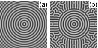
Figure 3: Domain patterns simulated by using the time-averaged model (14) without a strong defect: (a) $\rho=0.69$, and $\rho=0.5$. The parameters for (a) and (b) correspond to those of Figs. 1(a) and 1(b), respectively.

Now, we consider how concentric-ring patterns appear around a strong defect in this system, employing the time-averaged model. Actually, the time-averaged model (14) without a strong defect can also produce concentric-ring patterns. If the initial condition is given as $\Phi(\bm{r}=0)=1$ at the center and $\Phi(\bm{r})=-1$ anywhere else, then concentric-ring patterns, as shown in Fig. 3, are demonstrated by the time-averaged model without a strong defect. The values of $\rho$ for Figs. 3(a) and 3(b) are given by $\rho=0.69$ and $\rho=5$, which correspond to those for Figs. 1(a) and 1(b), respectively. One sees that Figs. 3(a) and 1(a) look very similar. They are observed near the threshold for nonuniform patterns, where the time-averaged model is valid. Near the threshold, the linear growth rate $\eta_{\bm{k}}$ given by Eq. (16) is very small, which means that the time scale of pattern formation is very slow. In fact, it takes more than 10 times longer time to obtain Fig. 3(a) than Fig. 3(b). If the initial pattern were completely uniform, nonuniform patterns could not appear easily. In other words, the initial condition employed here causes concentric rings on a uniform initial pattern (except for the center) as one of the simplest patterns. This situation is very similar to that of Fig. 1(a): The strong defect in the original model behaves as a kind of boundary condition in the almost uniform pattern near the threshold. Since the growth rate of the instability is very slow near the threshold, no patterns except for concentric rings can grow for Figs. 3(a) or 1(a). The growth rate is expected to be relevant to the correlation length, which is related to the number of concentric rings. From analogy with critical phenomena, one can estimate that the correlation length would be proportional to $\eta_{k_{0}}^{-1/2}$, where $\eta_{k_{0}}=\eta_{k=k_{0}}$. Therefore, the correlation length diverges near the threshold, as $\eta_{k_{0}}\to 0$. This is the mechanism of the emergence of a concentric-ring pattern around a strong defect and also the reason why the boundaries of the concentric-ring-pattern region are unclear in the phase diagram in Fig. 1.

In contrast, Fig. 3(b) has a few concentric rings, although stripes (or mazes) spread outside the rings. The stripes grow independently from the concentric rings because of rather large $\eta_{\bm{k}}$’s. The difference between Figs. 3(b) and 1(b) comes out not only because the time-averaged model is invalid far from the threshold, but also because the initial condition employed here is pretty different from the situation for Fig. 1(b).

The time-averaged model is also invalid for low frequencies. This is evident from Fig. 1 in which the theoretical threshold line is not consistent with the numerical one for $\omega/2\pi\lesssim 0.5$. The failure of the time-averaged model in a low-frequency region comes from the assumption $\phi(\bm{r},t)=\phi_{0}+\Phi(\bm{r},t)$. The assumption is valid when the time scales of the rapidly oscillating part and the slowly varying part are well separated. For low frequencies, their separation is not sufficient. If a multi-time-scale technique were applied, a better theoretical threshold line would be obtained.

The concentric-ring patterns shown in this paper are purely numerical results, although they suggest a possible mechanism about the formation of the patterns. Since the characteristics of domain patterns strongly depends on experimental conditions and samples, it is rather hard to compare experimental data with the results obtained in this paper. However, we can suggest that concentric-ring patterns appear in a certain range of the field strength and frequency, which is located above a labyrinth-pattern region. In fact, also in experiments, spirals and concentric rings are often observed near the threshold of nonuniform patterns kandaurova ; mino_p , although they are not always centered at a strong defect but often move around. Incidentally, for typical ferromagnetic garnet films, the order of the characteristic domain width is about 10-100 $\mu{\rm m}$ and that of the frequency for lattices, spirals, or concentric rings is about 0.1-100 kH kandaurova ; mino_p .

V Conclusions

In this paper, effects of an oscillating field have been investigated, and the emergence of concentric-ring patterns surrounding a strong defect has been discussed. The numerical simulations show that the concentric-ring pattern appears in the high-frequency region near the threshold for nonuniform patterns. The simulated profiles of the concentric-ring pattern indicate that the pattern consists of two parts (except for the vicinity of the defect) : A rapidly oscillating spatially homogeneous part and a nonuniform pattern part. This fact assures that the time-averaged model is suitable for the theoretical analysis. The theoretical threshold line is in good agreement with the numerical one in a high-frequency region. When the rapidly oscillating field makes the state close to the threshold, the concentric-ring pattern appears due to the strong defect which is an effective boundary condition.

In conclusion, the validity of the time-averaged model has been demonstrated in the presence of a rapidly oscillating filed. It gives the good estimate of the threshold for nonuniform patterns when the field frequency is high. Moreover, it is revealed that ideal and interesting patterns such as concentric-ring patterns can appear near the threshold, depending on boundary conditions.

- (1) L.D. Landau and E.M. Lifshitz, Mechanics (Pergamon, Oxford, 1960).
- (2) S. Rahav, I. Gilary, and S. Fishman, Phys. Rev. Lett. 91, 110404 (2003); Phys. Rev. A 68, 013820 (2003).
- (3) S. Rahav, E. Geva, and S. Fishman, Phys. Rev. E 71, 036210 (2005).
- (4) H. Saito and M. Ueda, Phys. Rev. Lett. 90, 040403 (2003).
- (5) F.K. Abdullaev, J.G. Caputo, R.A. Kraenkel, and B.A. Malomed, Phys. Rev. A 67, 013605 (2003).
- (6) C.N. Liu, T. Morishita, and S. Watanabe, Phys. Rev. A 75, 023604 (2007).
- (7) K. Kudo and K. Nakamura, Phys. Rev. E 76, 036201 (2007); AIP Conf. Proc. 1076, 129 (2008).
- (8) M. Cross and P.C. Hohenberg, Rev. Mod. Phys. 65, 851 (1993).
- (9) M. Seul and D. Andelman, Science 267, 476 (1995).
- (10) C.B. Muratov, Phys. Rev. E 66, 066108 (2002).
- (11) S. Miura, M. Mino and H. Yamazaki, J. Phys. Soc. Jpn. 70, 2821 (2001).
- (12) M. Mino, S. Miura, K. Dohi and H. Yamazaki, J. Magn. Magn. Mater. 226-230, 1530 (2001).
- (13) N. Tsukamoto, H. Fujisaka, and K. Ouchi, Prog. Theor. Phys. 161, 372 (2006).
- (14) G.S. Kandaurova, Phys. Usp. 45, 1051 (2002).
- (15) M. Mino (private communication).
- (16) D. Michaelis, F.Kh. Abdullaev, S.A. Darmanyan, and F. Lederer, Phys. Rev. E 71, 056205 (2005).
- (17) A.S. Kirakosyan, F.Kh. Abdullaev, and R.M. Galimzyanov, Phys. Rev. B 65, 094411 (2002).
- (18) L. Dong, F. Liu, S. Liu, Y. He, and W. Fan, Phys. Rev. E 72, 046215 (2005).
- (19) K.B. Migler and R.B. Meyer, Phys. Rev. Lett. 66, 1485 (1991).
- (20) S.V. Kiyashko, L.N. Korzinov, M.I. Rabinovich, and L.S. Tsimring, Phys. Rev. E 54, 5037 (1996).
- (21) J.R. de Bruyn, B.C. Lewis, M.D. Shattuck, and H.L. Swinney, Phys. Rev. E 63, 041305 (2001).
- (22) J.A. Tuszyński, M. Otwinowski, and J.M. Dixon, Phys. Rev. B 44, 9201 (1991).
- (23) E. A. Jagla, Phys. Rev. E 70, 046204 (2004).
- (24) K. Kudo, M. Mino, and K. Nakamura, J. Phys. Soc. Jpn. 76, 013002 (2007); K. Kudo and K. Nakamura, Phys. Rev. B 76, 054111 (2007).