This article is composed of two parts; In the first part (Sec. 1), the ultra-large-scale electronic structure theory is reviewed for (i) its fundamental numerical algorithm and (ii) its role in nano-material science. The second part (Sec. 2) is devoted to the mathematical foundation of the large-scale electronic structure theory and their numerical aspects.

1 Large-scale electronic structure theory and nano-material science

1.1 Overview

Nowadays electronic structure theory gives a microscopic foundation of material science and provides atomistic simulations in which electrons are treated as wavefunction within quantum mechanics. An example is given in the upper left panel of Fig.1. For years, we have developed fundamental theory and program code for large-scale electronic structure calculations, particularly, for nano materials. [1-6] The code was applied to several nano materials with $10^{2}$-$10^{7}$ atoms, whereas standard electronic structure calculations are carried out typically with $10^{2}$ atoms. Two application studies, for silicon and gold, are shown in the right panels and the lower left panels of Fig.1, respectively. Now the code is being reorganized as a simulation package, named as ELSES (Extra-Large-Scale Electronic Structure calculation), for a wider range of users and applications in science and industry. [6]

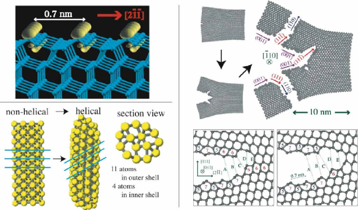
Figure 1: Upper left panel: Example of calculated electronic wavefunction on a silicon surface (A ‘$\pi$-type’ electron state on Si(111)-2x1 surface, given by a standard electronic structure calculation). Right panels: Application of our code to fracture dynamics of silicon crystal. [2] In results, the fracture path is bent into experimentally-observed planes (right upper panels) and and reconstructed Si(111)-2x1 surfaces appear with step formation (right lower panels). Lower left panels: Application of our code to formation process of helical multishell gold nanowire [5] that was reported experimentally. [7] A non-helical structure is transformed into a helical one (left and middle panels). The section view (right panel) shows a multishell structure, called ‘11-4 structure’, in which the outer and inner shells consist of eleven and four atoms, respectively.

1.2 Methodology

Our methodologies contain several mathematical theories, as Krylov-subspace theories for large sparse matrices. Here we focus on a solver method of shifted linear equations, called ‘shifted conjugate-orthogonal conjugate-gradient (COCG) method’ [3][4]. A quantum mechanical calculation within our studies is conventionally reduced to an eigen-value problem with a real-symmetric $N\times N$ matrix $H$ (Hamiltonian matrix), which will cost an $O(N^{3})$ computational time. In our method, instead, the problem is reduced to a set of shifted linear equations;

$$(z^{(k)}I-H)\,\,\bm{x}(z^{(k)})=\bm{b}$$ (1)

with a set of given complex variables $\{z^{(1)},z^{(2)},....z^{(L)}\}$ that have physical meaning of energy points. See Sec. 2 for mathematical foundation. Since the matrix $(z^{(k)}I-H)$ is complex symmetric, one can solve the equations by the COCG method, independently among the energy points. [8] In these calculations, the procedure of matrix-vector multiplications governs the computational time.

For the problem of Eq.(1), a novel Krylov-subspace algorithm, the shifted COCG method, was constructed [3][4], in which we should solve the equation actually only at one energy point (reference system). The solutions of the other energy points (shifted systems) can be given without any matrix-vector multiplication, which leads to a drastic reduction of computational time. The key feature of the shifted COCG method stems from the fact that the residual vectors $\bm{r}^{(k)}\equiv(z^{(k)}I-H)\bm{x}(z^{(k)})-\bm{b}$ are collinear among energy points, owing to the theorem of collinear residuals. [9]

Moreover, the shifted COCG method gives another drastic reduction of computational time, when one does not need all the elements of the solution vector $\bm{x}(z^{(k)})$, as in many cases of our studies. [3] For example, the inner product

$$\rho(\bm{b},z^{(k)})\equiv(\bm{b},\bm{x}(z^{(k)}))$$ (2)

is particularly interested in our cases. The shifted COCG method gives an iterative algorithm for the scaler $(\bm{b},\bm{x}(z^{(k)}))$, without calculating the vector $\bm{x}(z^{(k)})$, among the shifted systems. The quantity of Eq.(2) is known as ‘local density of states’ (See Sec. 2). It is an energy-resolved electron distribution at a point in real space and can be measured experimentally as a bias-dependent image of scanning tunneling microscope (See textbooks of condensed matter physics).

2 Note on mathematical formulation

Here a brief note is devoted to mathematical relationship between eigen-value equation and shifted linear equation in the electronic structure theory. A notation, known as bra-ket notation in quantum mechanics, is used. See Appendix for the details of the notation.

2.1 Original problem

Our problem in electronic structure calculation is, conventionally, reduced to an eigen-value problem, an effective Schrödinger equation,

$$H|v_{\alpha}\rangle=\varepsilon_{\alpha}|v_{\alpha}\rangle,$$ (3)

where $H$ is a given $N\times N$ real-symmetric matrix, called Hamiltonian matrix. Eigen vectors form a complete orthogonal basis set;

$$\langle v_{\alpha}|v_{\alpha}\rangle=\delta_{\alpha\beta}$$ (4)

$$\sum_{\alpha}|v_{\alpha}\rangle\langle v_{\alpha}|=I$$ (5)

where $I$ is the unit matrix.

In actual calculation, the matrix $H$ is sparse. Each basis of the matrix and the vectors corresponds to the wavefunction localized in real space. Hereafter physical discussion is given in the case that the physical system has $N$ atoms and only one basis is considered for one atom. In short, the $i$-th basis ($i=1,2,3...N$) corresponds to the basis localized on the $i$-th atom. Moreover we suppose, for simplicity, that the eigen values are not degenerated ($\varepsilon_{1}<\varepsilon_{2}<\varepsilon_{3}......$).

On the other hand, the linear equation of Eq. (1) is rewritten in the present notation;

$$(z-H)|x_{j}(z)\rangle=|j\rangle$$ (6)

with a complex valuable $z\equiv\varepsilon+i\eta$. The valuable $z$ corresponds to the energy with a tiny imaginary part $\eta$ ($\eta\rightarrow+0$).

The purpose within the present calculation procedure is to obtain selected elements of the following matrix $D$;

$$D(\varepsilon)\equiv\delta(\varepsilon-H)=\sum_{\alpha}|v_{\alpha}\rangle\delta(\varepsilon-\varepsilon_{\alpha})\langle v_{\alpha}|$$ (7)

or

$$D_{ij}(\varepsilon)=\sum_{\alpha}\langle i|v_{\alpha}\rangle\delta(\varepsilon-\varepsilon_{\alpha})\langle v_{\alpha}|j\rangle.$$ (8)

This matrix is called density-of-states (DOS) matrix, since its trace

$${\rm Tr}[D(\varepsilon)]=\sum_{\alpha}\delta(\varepsilon-\varepsilon_{\alpha}),$$ (9)

is called density of states. The physical meaning of Eq. (9) is the spectrum of eigen-value distribution.

In actual numerical calculation, the delta function in Eqs. (7) and (8) is replaced by an analytic function, a ‘smoothed’ delta function, since numerical calculation should be free from the singularity of the exact delta function ($\delta(0)=\infty$). The ‘smoothed’ delta function is defined as

$$\delta_{\eta}(\varepsilon)\equiv-\frac{1}{\pi}{\rm Im}\left[\frac{1}{\varepsilon+i\eta}\right]=\frac{1}{\pi}\frac{\eta}{\varepsilon^{2}+\eta^{2}}$$ (10)

with a finite positive value of $\eta(>0)$. The smoothed delta function gives the exact delta function in the limit of

$$\lim_{\eta\rightarrow+0}\delta_{\eta}(\varepsilon)=\delta(\varepsilon).$$ (11)

The physical meaning of $\eta$ is the width of the ‘smoothed’ delta function $\delta_{\eta}(\varepsilon)$. Hereafter, the DOS matrix is defined as

$$D(\varepsilon)\equiv\delta_{\eta}(\varepsilon-H)=\sum_{\alpha}|v_{\alpha}\rangle\delta_{\eta}(\varepsilon-\varepsilon_{\alpha})\langle v_{\alpha}|$$ (12)

or

$$D_{ij}(\varepsilon)=\sum_{\alpha}\langle i|v_{\alpha}\rangle\delta_{\eta}(\varepsilon-\varepsilon_{\alpha})\langle v_{\alpha}|j\rangle.$$ (13)

It is noteworthy that the smoothed delta function has a finite maximum

$$\delta_{\eta}(0)=\frac{1}{\eta}$$ (14)

and its integration gives the unity

$$\int_{-\infty}^{\infty}\delta_{\eta}(\varepsilon)d\varepsilon=\frac{1}{\pi}\left[{\rm tan}^{-1}\left(\frac{\varepsilon}{\eta}\right)\right]_{\varepsilon=-\infty}^{\varepsilon=\infty}=1.$$ (15)

2.2 Green’s function and calculation procedure

The Green’s function is defined as an inverse matrix of

$$G(z)\equiv\frac{1}{z-H}=\sum_{\alpha}\frac{|v_{\alpha}\rangle\langle v_{\alpha}|}{z-\varepsilon_{\alpha}}.$$ (16)

The solution of Eq. (6) gives the Green’s function;

$$G_{ij}(z)\equiv\langle i|G(z)|j\rangle=\langle i|x_{j}(z)\rangle$$ (17)

and the DOS matrix is given from the Green’s function;

$$D(\varepsilon)=-\frac{1}{\pi}{\rm Im}\left[G(\varepsilon+i\eta)\right],$$ (18)

under the relations of Eq. (10). In conclusion, the calculation procedure, from the Hamiltonian matrix to the DOS matrix, is illustrated, as follows;

$$H\stackrel{{\scriptstyle(\ref{EQ-SHIFTED-LE})(\ref{EQ-X-G})}}{{\Longrightarrow}}G\stackrel{{\scriptstyle(\ref{EQ-G-D})}}{{\Longrightarrow}}D$$ (19)

2.3 Physical quantities for energy decomposition

Now we present two quantities, local density of states (LDOS) and crystal orbital Hamiltonian population (COHP)[10], as examples of important physical quantities that is calculated from selected element of the DOS matrix. These quantities appear in the decomposition methods of the electronic structure energy. The electronic structure energy is defined as

$$E=\sum_{\alpha}\varepsilon_{\alpha}f(\varepsilon_{\alpha}),$$ (20)

where $f(\varepsilon_{\alpha})$ is the number of electrons that occupy the wavefunction with the energy of $\varepsilon_{\alpha}$. In the present case, the case of zero temperature, the function is reduced to a step-function form of

$$f(\varepsilon)\equiv\theta(\mu-\varepsilon)$$ (21)

with a given value of $\mu$ (chemical potential). Eqs.(20), (9) lead us to the expression of the energy with DOS;

$$E = \int_{-\infty}^{\infty}f(\varepsilon)\,\varepsilon\,\sum_{\alpha}\delta(\varepsilon-\varepsilon_{\alpha})\,d\varepsilon$$ (22)

$$= \int_{-\infty}^{\infty}f(\varepsilon)\,\varepsilon\,{\rm Tr}[D(\varepsilon)]\,d\varepsilon$$

2.3.1 Decomposition with local density of states

LDOS is defined as diagonal elements

$$n_{i}(\varepsilon)\equiv\langle i|D(\varepsilon)|i\rangle=\sum_{\alpha}|\langle i|v_{\alpha}\rangle|^{2}\delta(\varepsilon-\varepsilon_{\alpha})$$ (23)

of the DOS matrix and the energy is decomposed into the contributions of LDOS, $\{n_{i}(\varepsilon)\}_{i}$;

$$E=\sum_{i}\int_{-\infty}^{\infty}f(\varepsilon)\varepsilon n_{i}(\varepsilon)d\varepsilon.$$ (24)

Physical meaning of LDOS is a weighted eigen-value distribution; For example, if an eigen vector $|v_{\alpha}\rangle$ has a large weight on the $i$-th basis, the local DOS $n_{i}(\varepsilon)$ has a large peak at the energy level of $\varepsilon=\varepsilon_{\alpha}$. The LDOS $n_{i}(\varepsilon)$ corresponds to the experimental image of the scanning tunneling microscope (See the end of Sec. 1).

2.3.2 Decomposition with crystal orbital Hamiltonian population

Another decomposition of the energy can be derived with an expression of

$$E=\int_{-\infty}^{\infty}f(\varepsilon){\rm Tr}[D(\varepsilon)H]d\varepsilon.$$ (25)

Eq.(25) is proved from the first line of Eq.(22) and the relation of

$${\rm Tr}[D(\varepsilon)H] = {\rm Tr}[\delta_{\eta}(\varepsilon-H)H]$$ (26)

$$= \sum_{\alpha}\langle\phi_{\alpha}|\delta_{\eta}(\varepsilon-H)H|\phi_{\alpha}\rangle$$

$$= \sum_{\alpha}\langle\phi_{\alpha}|\delta_{\eta}(\varepsilon-\varepsilon_{\alpha})\varepsilon_{\alpha}|\phi_{\alpha}\rangle$$

$$= \sum_{\alpha}\delta_{\eta}(\varepsilon-\varepsilon_{\alpha})\varepsilon_{\alpha}$$

$$= \varepsilon\sum_{\alpha}\delta_{\eta}(\varepsilon-\varepsilon_{\alpha}).$$

The last equality is satisfied by the exact delta function ($\eta\rightarrow 0+$). Eq.(25) gives another decomposition of the energy

$$E=\sum_{ij}\int_{-\infty}^{\infty}f(\varepsilon)C_{ij}(\varepsilon)d\varepsilon,$$ (27)

where the matrix $C$ is defined as

$$C_{ij}(\varepsilon)\equiv D_{ij}(\varepsilon)H_{ji}$$ (28)

and is called crystalline orbital Hamiltonian population (COHP) [10]. The physical meaning of COHP is an energy spectrum of electronic wavefunctions, or ‘chemical bond’, that lie between $i$-th and $j$-th bases. See the papers [3, 10] for details.

2.4 Numerical aspects with Krylov subspace theory

Several numerical aspects are discussed for the calculated quantities within Krylov subspace theory, such as the shifted COCG algorithm. LDOS is focused on, as an example. When we solve the shifted linear equation of Eq. (6) within the $\nu$-th order Krylov subspace

$$K^{(\nu)}(H;|j\rangle)\equiv{\rm span}\left\{|j\rangle,H|j\rangle,H^{2}|j\rangle,......,H^{\nu-1}|j\rangle\right\},$$ (29)

the resultant LDOS should include deviation from the properties in the previous sections, properties of the exact solution.

First, the number of peaks in the LDOS function ($n_{i}(\varepsilon)$) is equal to $\nu$, the dimension of Krylov subspace, whereas the number of peaks in the exact solution, given in Eq.(23) is $N$, the dimension of the original matrix. A typical behavior is seen Fig.3(a) of Ref.[3], a case with $\nu=30$ and $N=1024$. Here we note that the calculation with such a small subspace ($\nu=30$) gives satisfactory results in several physical quantities [3], mainly because many physical quantities are defined by a contour integral with respect to the energy, as in Eq. (22), and the information of individual peaks is not essential.

Second, the calculated function $n_{i}(\varepsilon)$ in the Krylov subspace can be negative $(n_{i}(\varepsilon)<0)$, whereas the exact one, given in Eq.(23), is always positive. In the exact solution of Eq.(23), peaks in $n_{i}(\varepsilon)$ are given by the poles of the Green’s function $G(z)$ ($z=\varepsilon_{1},\varepsilon_{2},....$) and the function $n_{i}(\varepsilon)$ contains smoothed delta functions of

$$\delta_{\eta}(\varepsilon-\varepsilon_{\alpha})\equiv-\frac{1}{\pi}{\rm Im}\left[\frac{1}{(\varepsilon-\varepsilon_{\alpha})+i\eta}\right].$$ (30)

Since $\varepsilon_{\alpha}$ is an eigen value of the real-symmetric matrix $H$ and is real $({\rm Im}[\varepsilon_{\alpha}]=0)$, the exact Green’s function $G(z)$ has poles only on real axis. In the calculation within Krylov subspace, however, the poles can be deviated from real axis ($\varepsilon_{\alpha}=\varepsilon_{\alpha}^{\rm(r)}+i\varepsilon_{\alpha}^{\rm(i)},\varepsilon_{\alpha}^{\rm(i)}\neq 0$). In that case, the sign of the smoothed delta function can be negative;

$$\delta_{\eta}(\varepsilon-\varepsilon_{\alpha}) \equiv -\frac{1}{\pi}{\rm Im}\left[\frac{1}{(\varepsilon-\varepsilon_{\alpha})+i\eta}\right]$$ (31)

$$= -\frac{1}{\pi}{\rm Im}\left[\frac{1}{(\varepsilon-\varepsilon_{\alpha}^{\rm(r)})+i(\eta-\varepsilon_{\alpha}^{\rm(i)})}\right]$$

$$= \frac{1}{\pi}\frac{\eta-\varepsilon_{\alpha}^{\rm(i)}}{(\varepsilon-\varepsilon_{\alpha}^{\rm(r)})^{2}+(\eta-\varepsilon_{\alpha}^{\rm(i)})^{2}}.$$

The above expression indicates that a negative peak appears ($\delta_{\eta}(\varepsilon-\varepsilon_{\alpha})<0$), when the imaginary part of a pole is larger than the value of $\eta$ ($\eta<\varepsilon_{\alpha}^{\rm(i)}$). Therefore, we can avoid the negative peaks, when we use a larger value of $\eta$, which was confirmed among actual numerical calculations with the shifted COCG algorithm.

Finally, we comment on the present discussion from the interdisciplinary viewpoints between physics and mathematics; From the mathematical view point, we can say that the above two numerical aspects disappear, when the dimension of the Krylov subspace ($\nu$) increases to be enough large. We would like to emphasis that, even if the dimension is rather small, we can obtain fruitful quantitative discussion for several physical quantities, as discussed above. In other words, mathematics gives a rigorous way (iterative solver) to the exact solution and physics gives a practical measurement of the convergence criteria.

Appendix A Notation used in Section 2

In Sec.2, we use the vector notations of

$$|f\rangle\Leftrightarrow(f_{1},f_{2}.....f_{M})^{\rm T}$$ (32)

$$\langle g|\Leftrightarrow(g_{1},g_{2}.....g_{M}).$$ (33)

Particularly, the unit vector of which non-zero component is only the $i$-th one is denoted as $|i\rangle$;

$$|i\rangle\Leftrightarrow(0,0,....,1_{i},0,0)^{\rm T}.$$ (34)

Inner products are described as

$$\langle g|f\rangle\equiv\sum_{i}g_{i}f_{i}$$ (35)

are

$$\langle g|A|f\rangle\equiv\sum_{ij}g_{i}A_{ij}f_{j}$$ (36)

with a $N\times N$ matrix $A$. The notation of $|f\rangle\langle g|$ indicates a matrix, of which a component is given as

$$\left(|f\rangle\langle g|\right)_{ij}=f_{i}g_{j}.$$ (37)

These notations are used in quantum mechanics and called ‘bra-ket’ notation. We should say, however, that the above notations are slightly different of the original ‘bra-ket’ notations. For example, the original notation of $\langle g|$ is $\langle g|\Leftrightarrow(g_{1}^{\ast},g_{2}^{\ast}.....g_{M}^{\ast})$. The reason of the difference comes from the fact that the standard quantum mechanics is given within linear algebra with Hermitian matrices but the present formulation is not.

References

- [1] http://fujimac.t.u-tokyo.ac.jp/lses/index.html; Our project page (CREST-JST project) with Prof. Takeo Fujiwara (University of Tokyo). The full publication list and several simulation results, as movie files, are available.
-
[2]
T. Hoshi, Y. Iguchi and T. Fujiwara,
Phys. Rev. B72, 075323 (2005).
Preprint: http://arxiv.org/abs/cond-mat/0611738 -
[3]
R. Takayama, T. Hoshi, T. Sogabe, S-L. Zhang and T. Fujiwara,
Phys. Rev. B73, 165108 (2006).
Preprint: http://arxiv.org/abs/cond-mat/0503394 -
[4]
T. Sogabe, T. Hoshi, S.-L. Zhang, and T. Fujiwara,
Frontiers of Computational Science, pp. 189-195,
Ed. Y. Kaneda, H. Kawamura and M. Sasai,
Springer Verlag, Berlin Heidelberg
(2007).
Preprint: http://arxiv.org/abs/math/0602652v1 -
[5]
Y. Iguchi, T. Hoshi and T. Fujiwara,
Phys. Rev. Lett. 99, 125507 (2007).
Preprint: http://arxiv.org/abs/cond-mat/0611738 - [6] http://www.elses.jp/; the ELSES consortium
- [7] Y. Kondo and K. Takayanagi, Science 289, 606 (2000).
- [8] H. A. van der Vorst and J. B. M. Melissen, IEEE Trans. Magn. 26, 706 (1990).
- [9] A. Frommer, Computing 70, 87 (2003).
- [10] R. Dronskowski, P.E. Blöchl, J. Phys. Chem. 97, 8617 (1993).