Stellar Populations in the Andromeda V Dwarf Spheroidal Galaxy

Abstract

Using archival imaging from the Wide Field Planetary Camera 2 aboard the Hubble Space Telescope, we investigate the stellar populations of the Local Group dwarf spheroidal Andromeda V - a companion satellite galaxy of M31. The color-magnitude diagram (CMD) extends from above the first ascent red giant branch (RGB) tip to approximately one magnitude below the horizontal branch (HB). The steep well-defined RGB is indicative of a metal-poor system while the HB is populated predominantly redward of the RR Lyrae instability strip. Utilizing Galactic globular cluster fiducial sequences as a reference, we calculate a mean metallicity of $[Fe/H]=-2.20\pm 0.15$ and a distance of $(m-M)_{0}=24.57\pm 0.04$ after adopting a reddening of $E(B-V)=0.16$. This metal abundance places And V squarely in the absolute magnitude - metallicity diagram for dwarf spheroidal galaxies. In addition, if we attribute the entire error-corrected color spread of the RGB stars to an abundance spread, we estimate a range of $\sim$0.5 dex in the metallicities of And V stars. Our analysis of the variable star population of And V reveals the presence of 28 potential variables. Of these, at least 10 are almost certainly RR Lyrae stars based on their time sequence photometry.

1. Introduction

Dwarf spheroidal and dwarf irregular galaxies are thought to be instrumental in the process that forms larger galaxies (Font et al. 2006, and references therein). As such, their importance is sometimes considered only within this context - that of much more massive systems. However, it is important to keep in mind that dwarf galaxies (DGs) are useful probes of galaxy formation and evolution in and of themselves. In this regard, the relation between the absolute magnitude of a DG and its mean metallicity has provided a number of useful insights. First studied decades ago (Tinsley 1978; Mould, Kristian, & Da Costa 1983), this relation shows that more luminous DGs possess a more metal-rich mean abundance. This in turn suggests that self-enrichment by heavy elements is more likely in a system with a larger gravitational potential which can retain supernova ejecta (e.g. Davidge et al. 2002).

Within the context of this mass-metallicity correlation, Andromeda V, a dwarf spheroidal companion galaxy to M31, is somewhat of an anomaly. In their discovery paper, Armandroff et al. (1998) used Milky Way globular cluster fiducials combined with V and I imaging to measure a mean metallicity for And V of $[Fe/H]=-1.5$. At its measured absolute magnitude of $M_{V}\sim-9$, we expect And V to have $[Fe/H]\sim-2$, similar to the Milky Way dSphs Ursa Minor and Draco, so the Armandroff et al. (1998) value made And V a significant outlier among the Local Group dwarf spheroidal galaxies in the relation between absolute magnitude and metallicity. This led Caldwell (1999) to hypothesize that perhaps And V has a deeper than normal potential well, which could be verified through measurements of its stellar velocity dispersion or mass-to-light ratio.

Motivated by the discrepancy between the expected and observed properties of And V, Davidge et al. (2002) re-examined the question of And V’s chemical composition. They used the Gemini Multi-Object Spectrograph (GMOS) in imaging mode on the Gemini North telescope to construct an optical color-magnitude diagram (CMD) in the g’, r’, and i’ filters. The slope of the And V red giant branch (RGB) was then used to calculate the mean metallicity of [Fe/H] = $-2.2\pm 0.1$ placing And V squarely on the $M_{V}-[Fe/H]$ relation. Davidge et al. (2002) therefore asserted that there was nothing unusual about the metallicity of And V and that the absolute integrated magnitude and metallicity do indeed follow the relation for dwarf spheroidal galaxies. However, this result was again thrown into doubt with the work of McConnachie et al. (2005). Using Johnson V and Gunn i photometry from the Isaac Newton Telescope Wide Field Camera they calculated $[Fe/H]=-1.6$ from the mean color of the And V RGB. This once again returned And V to the status of an outlier in the $M_{V}-[Fe/H]$ relation.

In light of the uncertainty about the mean abundance of stars in And V, and the overall importance of characterizing the properties of stars in dwarf spheroidal galaxies, we have undertaken a photometric study of And V using archival imaging from the Hubble Space Telescope (HST) Wide FIeld Planetary Camera 2 (WFPC2). In section 2 we detail our observations and reductions, while section 3 presents the color-magnitude diagram (CMD) of And V along with a discussion of its properties; our conclusions are summarized in Sec. 4.

2. Observations and Reductions

The images used in the present study are archival WFPC2 observations of And V as detailed in Table 1. The observations, taken as part of program GO-8272 (PI: Armandroff) consist of 16 F450W and 8 F555W images. Due to a malfunction in the observing sequence, the images were taken at two different times – half were taken in November of 1999 and half in December of 2000. The first and second set of 12 observations each cover a time baseline of approximately half of a day. There is a slight rotational offset between the two observations as illustrated by Fig. 1, which shows a $12$ x $12$ arcmin digitized sky survey image of And V with the WFPC2 footprint outlined.

All of the program frames were reduced using the HSTphot software (Dolphin 2000) package. First, all of the required preliminary steps were performed such as masking the cosmic rays and the hot pixels, as well as calculating the background sky contribution to each pixel. Then, the stellar photometry was performed on the processed images. HSTphot detects stars and fits TINY TIM point spread functions to the detected profiles. It also applies geometric, charge transfer efficiency, and aperture corrections to the resultant magnitudes. The instrumental photometry is then calibrated to standard Johnson-Cousins BV magnitudes (for details see Dolphin 2000). It is important to note that the validity and robustness of Dolphin’s (2000) photometry software and his characterization of WFPC2’s photometric performance have been verified by Sirianni et al. (2005).

HSTPhot is able to photometer multiple images simultaneously as long as they share the same rotational orientation. It calculates positional offsets between the frames, matches the stars and outputs average magnitudes in each filter. We applied this process to the two sets of images (one set at each rotation) and found small offsets between them ($\Delta$B = 0.028, $\Delta$V = 0.010). We then offset each set of data to the mean photometric zeropoint and combined measurements of stars in common between the two rotations. The final list contains stars that were detected on at least 12 different frames between the two rotations.

3. Results

3.1. The Color Magnitude Diagram

The CMD of And V, shown in Fig. 2, extends from above the first ascent RGB tip to roughly 1 magnitude below the horizontal branch (HB). The relatively steep RGB argues in favor of And V being fairly metal-poor, while at the same time, the predominantly red HB suggests a somewhat younger age (Stetson et al. 1999; Da Costa et al. 2002). We will explore these issues in more detail below. There is evidence for foreground contamination from the Milky Way on both sides of the RGB. Simulations using the Besancon Galaxy model (Robin et al. 2003) confirm that these are indeed Milky Way foreground stars as illustrated in Fig. 3 wherein the open triangles represent the model foreground stars. These simulations also suggest the absence of a significant intermediate-age (2 to 8 Gyr) population in And V due to the lack of asymptotic giant branch (AGB) stars located above the RGB tip (Martinez-Delgado & Aparicio 1997; Martinez-Delgado et al. 1999). That is to say, the number of such AGB stars is consistent with the degree of field contamination. This finding is in-line with that of Davidge et al. (2002) who reached the same conclusion based on their ground-based GMOS CMD.

3.2. Metallicity from the Red Giant Branch

A statistically significant spread in the colors of And V RGB stars would suggest the presence of a range of ages and/or metallicities in this system. Given the lack of AGB stars above the first ascent tip and the relative insensitivity of RGB colors to age as compared with metallicity, it is more likely that a range in the colors of RGB stars is a reflection of a spread in metal abundance among the stars in And V. We can quantify this dispersion along with the mean [Fe/H] by using Milky Way globular cluster RGB fiducials. For this, we make use of the sequences for M15, NGC 6752, NGC 1851, and 47 Tucanae published by Sarajedini & Layden (1997) and plotted in Fig. 3. These clusters have metal abundances of –2.17, –1.54, –1.29, and –0.71, respectively, on the Zinn & West (1984) scale. We have adopted the Chaboyer (1999) relation between HB magnitude and metallicity - $M_{V}(HB)=0.23[Fe/H]+0.93$.

The next step is to produce a locus of points to represent the mean RGB of And V. To expedite this, we divide the RGB stars brighter than $V=25$ into bins of 0.2 mag. For each bin, we used a 2-$\sigma$ rejection algorithm to calculate the mean B–V color. The resultant RGB locus is used to calculate the mean abundance of And V via the procedure described by Da Costa et al. (2000). This method uses the relationship between metal abundance and mean HB magnitude to calculate a distance modulus based on an initial guess of the metal abundance; the distance is used to place the fiducials in the CMD and measure the mean metallicity, which is again used to calculate a new distance. This is an iterative process, but quickly converges after only a few calculations. To determine the mean HB mag of And V, we also follow the lead of Da Costa et al. (2000) by selecting stars between $25.25<V<25.65$ and $-0.05<B-V<0.4$, which gives $\langle$V(HB)$\rangle$$=25.49\pm 0.01$ (standard error of the mean). Adopting a reddening of E(B–V)= 0.16 (Burstein & Heiles, 1982), this process yields a distance of $(m-M)_{0}=24.57\pm 0.04$ and a mean metallicity of $[Fe/H]=-2.20\pm 0.15$ for And V. The errors are calculated by shifting the HB by its error and the RGB by the mean color error in bins of 0.2 mag and then redoing the analysis. The resultant differences in the distance modulus and the metallicity are then the adopted errors in these quantities.

We will quantify the HB morphology in the next section, but for now, it is important to note that with such a low metallicity and a HB that is predominantly redward of the RR Lyrae instability strip, And V represents an extreme case of the second parameter effect. This has been noted by Harbeck et al. (2001) in their study of this galaxy which makes use of the same observational material we present here. If we assume that the red HB morphology of And V is primarily a result of relative youth, then we can place some limits on how our derived mean metal abundance will change as a result. As noted above, the lack of a significant supra-RGB-tip AGB population suggests that the dominant population in And V is older than $\sim$8 Gyr. Yet, based on the ages and HB morphologies of the Galactic globulars, the oldest of which have ages of around 13 Gyr, And V must be $\sim$3 Gyr younger than globular clusters at its metal abundance. Hence, we estmate an age between 8 and 10 Gyr for the majority of stars in And V. This would make our quoted mean abundance value of $[Fe/H]=-2.20\pm 0.15$ more metal-rich by $\sim$0.1 dex according to the theoretical models of Dotter et al. (2007).

Moving on to the metallicity spread in And V, Fig. 5 shows the color spread of And V stars around our adopted fiducial sequence (solid line in Fig. 4) for stars in the range $23<V<24$. A gaussian fit to these data yields a 1-$\sigma$ color spread of 0.076 mag, which becomes 0.070 mag after the mean photometric error of 0.031 mag is subtracted in quadrature. We note that this mean error as given by HSTphot is consistent with the dispersion in the magnitudes of the same stars measured at the two rotations. Using the globular cluster fiducials plotted in Fig. 4, we can use the dereddened color of these sequences at $M_{V}=-1.5$, the approximate middle of the magnitude range of RGB stars we are considering, as a function of abundance to translate a color range of 0.070 mag to a metal abundance spread of 0.52 dex.

Converting the intrinsic color spread to a metallicity spread is complicated by two effects. First, there is the possibility that some of the color spread is caused by a range of ages among the And V stellar population. However, as discussed above, based on the lack of a young main sequence and AGB stars above the first ascent RGB tip, and the relative insensitivity of RGB colors to age, we expect this effect to be be small. Second, there is the problem of needing to extrapolate the globular cluster fiducials to more metal-poor regimes in order to convert the RGB color spread to an abundance spread. Both of these effects will introduce a level of uncertainty into our metallicity spread determination.

3.3. Horizontal Branch Morphology

It is clear from the CMD of And V that this galaxy has a primarily red HB, one explanation of which is the presence of a substantial young population. To quantify the HB morphology of And V, we follow the procedure outlined in Da Costa et al. (2000) for calculating the index $i=b/(b+r)$, where b and r represent the number of stars on the blue and red sides of the RR Lyrae instability strip, respectively. This method was originally developed for their work on And I and And II (Da Costa et al. 1996, Da Costa et al. 2000). In the case of those two companion galaxies, one set of HB color and magnitude limits was used. However the lower metallicity of And III and And V shifts their RGBs to the blue, introducing RGB contamination into the HB if the same color limits are used. To circumvent this difficulty for And III, the HB morphology index was measured by Da Costa et al. (2002) using two different methods - a procedure that we also adopt here.

For the first calculation, a color histogram is created for the stars on the HB ($25.25<F555W<25.65$). This histogram exhibits a sharp decline redward of approximately $F450W-F555W=0.5$, as was the case for Andromeda III. We take this to be the point at which RGB stars begin to dominate over the HB stars. We then take the red stars to be those between these magnitude limits and between the colors $0.35<F450W-F555W<0.5$, and find that $r=339$. Next we use the same magnitude range for the blue stars and use color limits of $-0.05<F450W-F555W<0.25$, finding $b=107$. Assuming errors due only to Poisson statistics, we find $i^{\prime}=0.24\pm 0.03$. The prime designates a value based on the And III color limits.

Our next approach involves using the same color limits as used with And I and And II - the red edge of the HB is placed at $F450W-F555W=0.60$ - and then correcting for RGB contamination by using the RGB density above and below the HB to estimate the number of contaminating stars. This yields $r=416$, $b=107$, and $i=0.20\pm 0.02$, in agreement with our initial estimate. Compared with values of $i=0.13\pm 0.01$, $0.18\pm 0.02$, and $0.10\pm 0.02$ for And I, And II, and And III, respectively, And V is on the blue end of the HB morphology scale for these dwarf galaxies, though it is similar to And III.

Another important point of investigation is the presence of a radial gradient in the HB morphology of And V. Previous searches for this effect have revealed a gradient in And I, but not in And II or And III. We have searched for a gradient in And V using the same methodology as Da Costa et al. (2000). First, adopting a core radius of 27.91” and zero eccentricity (Caldwell 1999), we divide the stars into two populations: those inside the core radius and those outside. We find $i^{\prime}=0.20\pm 0.07$ and $i=0.11\pm 0.03$ for the inner population and $i^{\prime}=0.24\pm 0.03$ and $i=0.23\pm 0.03$ for the outer population. Next we divide the stars in And V at a distance of 52” to yield two equal-sized samples. For these two populations we find $i^{\prime}=0.24\pm 0.04$ and $i=0.17\pm 0.03$ for the inner stars and $i^{\prime}=0.24\pm 0.03$ and $i=0.24\pm 0.03$ for the outer stars. The primary conclusion from this exercise is that if there is a radial gradient in the HB morphology of And V, it is too small to be reliably detected. This lack of a population gradient is in agreement with the results of Harbeck et al. (2001).

3.4. Characterization of Variable Stars

To identify the variable stars in And V we created an initial candidate list for each rotation separately. To be considered as a candidate, a star had to be detected in every exposure of a given rotation and exhibit a frame-to-frame standard deviation of $\geq$0.2 mag. We then examined the raw light curves of the resulting candidates from each rotation to identify potential RR Lyrae stars. This process provided a total of 28 RR Lyrae candidates. When available, the photometric data from the other rotation was then added to the dataset and used as input into our period finding routine. Ten candidates had data from both observing windows. These ten variables have $<$V$>$ = 25.55 and $<$B-V$>$ = 0.30 putting them in the middle of the HB, which combined with the shapes of their raw light curves unambiguously identifies them as RR Lyraes. We therefore refer to these 10 RR Lyraes as our high confidence variables. The other 18 candidates are also likely to be RR Lyraes but due to poor phase coverage we can’t exclude the possibility that they are another type of variable. These form our set of candidate variables. Tables 2-7 show the raw magnitude measurements at each epoch for all variables. Table 3 lists RA and Dec for the high confidence variables. The locations of the high confidence variables in the CMD are shown in Fig. 3. Table 4 lists positions for the candidate variables.

We attempted to measure periods for our high confidence variables by using a template fitting method similar to that of Layden (1998). We iterated with a step size of 0.0001 days over the range of periods from 0.2-1.5 days, and at each point used Pikaia (Charbonneau 1995) to find the combination of epoch, amplitude, and mean magnitude that minimized the $\chi$² differences between the observed data points and 10 variable star templates taken from the work of Layden (1998). Pikaia was then run once more with period as an additional free parameter, allowing it to search within $\pm$0.0001 days of the best fitting period from the inital search. This refinement step provided our best guess for the period of each variable. As a check of our results a series of statistical simulations were performed in which artificial RR Lyraes were created with the same photometric errors and observing cadence as the observations, and then fitted in the same manner as our high confidence variables. These simulations demonstrated that our template fitting algorithm couldn’t robustly derive periods for the variables. Unfortunately, this result is not a limit of our algorithm but a result of the spacing of the observations. The longest contiguous observing window in a single filter is only 0.4 days, too short to accurately measure the likely periods of the AB-type RR Lyraes (0.5-0.8 days). Although we cannot measure periods for these variables we include figure 6, a plot of the raw and folded light curves for high confidence variable 8, to demonstrate the RR Lyrae nature of these variables. The parameters of the fit come from our template fitting algorithm. The fitted parameters for this variable are $<$B$>$ = 25.87, $<$V$>$ = 25.31, B amplitude = 1.03, V amplitude = 0.83, a period of 0.785235 days, and a starting epoch of 2451496.04345703 (HJD). This variable demonstrates the typical quality of the raw and fitted light curves for the high confidence variables.

4. Summary and Conclusions

This work presents HST WFPC2 F450W and F555W observations of Andromeda V, a dwarf spheroidal galaxy satellite of M31. Comparing the CMD of And V to Milky Way Globular cluster fiducials of known metallicity, we find a mean metal abundance for And V of $[Fe/H]=-2.20\pm 0.15$ with a spread of $\sim$0.5 dex, and a distance modulus of $(m-M)_{0}=24.57\pm 0.04$. This result puts Andromeda V squarely on the absolute magnitude - metallicity relationship for local group dwarf spheroidals. As suggested by Davidage et al. (2004) this tightens the relationship between absolute magnitude and metallicity, suggesting that there is little scatter in the relationship between mass-to-light ratio and absolute magnitude for dwarf spheroidals. In addition we find RR Lyraes in And V providing evidence for an old population, but are unable to accurately measure their periods.

Table 1Observing Log

Date	Dataset	Filter	Exp Time
November 11, 1999	U5C701	F555W	3 x 1200s
November 12, 1999	U5C701	F450W	8 x 1200s
November 13, 1999	U5C702	F555W	1 x 1300s
December 16, 2000	U5C752	F555W	1 x 1200s
December 17, 2000	U5C752	F555W	3 x 1200s
December 17, 2000	U5C752	F450W	8 x 1300s

Table 2Observed Light Curves For Variables 01-05

Filter	HJD	01 Mag	01 Err	02 Mag	02 Err	03 Mag	03 Err	04 Mag	04 Err	05 Mag	05 Err
V	2451494.37626	25.42	0.093	25.33	0.083	25.69	0.111	25.54	0.100	25.23	0.076
V	2451494.39432	25.61	0.114	25.15	0.077	25.83	0.129	25.71	0.118	25.16	0.079
V	2451494.44154	25.61	0.110	25.63	0.105	25.64	0.106	25.36	0.086	25.36	0.085
V	2451494.50821	25.88	0.135	25.71	0.112	$\cdots$	$\cdots$	25.37	0.087	25.43	0.114
B	2451494.57614	26.51	0.255	$\cdots$	$\cdots$	$\cdots$	$\cdots$	25.55	0.118	26.28	0.173
B	2451494.64350	26.72	0.306	25.45	0.108	25.55	0.114	25.71	0.135	26.08	0.148
B	2451494.71017	26.48	0.253	25.52	0.115	25.73	0.130	25.66	0.128	26.20	0.189
B	2451494.77753	25.87	0.149	25.83	0.143	26.15	0.177	25.84	0.146	26.52	0.207
B	2451494.84420	25.48	0.120	26.12	0.244	26.34	0.205	25.44	0.108	26.46	0.199
B	2451494.91156	25.55	0.116	25.56	0.116	26.09	0.169	25.24	0.092	25.66	0.134
B	2451494.93031	25.84	0.150	25.56	0.120	26.50	0.252	25.43	0.110	25.43	0.093
B	2451494.97892	26.17	0.190	25.50	0.114	25.90	0.147	25.68	0.129	25.95	0.169
V	2451895.46983	25.64	0.116	25.56	0.104	25.38	0.091	25.28	0.078	25.76	0.118
V	2451895.53511	25.65	0.121	25.17	0.079	25.50	0.113	25.62	0.156	25.62	0.109
V	2451895.60177	25.53	0.109	25.44	0.096	25.89	0.139	25.66	0.105	25.69	0.116
V	2451895.66914	24.91	0.068	25.84	0.134	25.55	0.106	25.82	0.125	25.54	0.103
B	2451895.73638	25.42	0.115	26.08	0.183	26.81	0.338	26.49	0.234	25.39	0.111
B	2451895.75513	25.49	0.109	26.03	0.160	26.31	0.222	26.31	0.185	25.28	0.094
B	2451895.80374	25.65	0.136	25.75	0.137	26.18	0.190	26.09	0.164	25.36	0.106
B	2451895.82249	25.74	0.132	25.50	0.106	26.19	0.174	25.82	0.132	25.57	0.116
B	2451895.87041	25.73	0.143	25.54	0.117	25.86	0.148	26.04	0.157	25.84	0.157
B	2451895.88916	26.03	0.167	25.96	0.151	25.91	0.144	25.94	0.139	25.64	0.122
B	2451895.93777	26.13	0.197	25.94	0.159	25.76	0.136	26.21	0.183	25.96	0.171
B	2451895.95652	26.13	0.181	26.11	0.167	25.54	0.107	26.28	0.183	25.94	0.154

Table 3Observed Light Curves For Variables 06-10

Filter	HJD	06 Mag	06 Err	07 Mag	07 Err	08 Mag	08 Err	09 Mag	09 Err	10 Mag	10 Err
V	2451494.37626	26.16	0.157	25.48	0.093	25.71	0.109	25.37	0.085	25.65	0.099
V	2451494.39432	26.10	0.157	25.58	0.107	25.68	0.115	25.32	0.084	25.67	0.107
V	2451494.44154	25.61	0.108	25.55	0.099	24.95	0.063	25.55	0.097	25.69	0.101
V	2451494.50821	25.36	0.107	$\cdots$	$\cdots$	$\cdots$	$\cdots$	25.60	0.119	25.76	0.108
B	2451494.57614	26.15	0.163	25.11	0.086	25.84	0.130	26.19	0.169	26.17	0.180
B	2451494.64350	26.55	0.209	25.39	0.105	26.07	0.158	26.37	0.191	25.92	0.148
B	2451494.71017	$\cdots$	$\cdots$	25.64	0.126	25.89	0.137	26.75	0.260	25.86	0.140
B	2451494.77753	26.92	0.286	25.72	0.133	26.01	0.151	26.29	0.187	25.12	0.081
B	2451494.84420	26.60	0.219	25.72	0.134	26.15	0.168	25.58	0.104	25.45	0.103
B	2451494.91156	$\cdots$	$\cdots$	$\cdots$	$\cdots$	26.27	0.188	25.89	0.130	25.61	0.116
B	2451494.93031	26.91	0.289	26.01	0.176	25.95	0.152	25.86	0.131	25.57	0.116
B	2451494.97892	26.74	0.258	25.91	0.153	$\cdots$	$\cdots$	25.87	0.127	26.13	0.172
V	2451895.46983	25.78	0.118	25.54	0.102	25.44	0.096	25.57	0.103	25.57	0.098
V	2451895.53511	25.95	0.138	25.57	0.107	25.42	0.098	25.39	0.094	25.61	0.104
V	2451895.60177	25.82	0.126	25.45	0.097	25.61	0.113	25.41	0.094	25.34	0.085
V	2451895.66914	26.03	0.152	25.52	0.104	25.29	0.090	25.16	0.079	$\cdots$	$\cdots$
B	2451895.73638	25.36	0.118	24.90	0.085	25.27	0.104	25.81	0.137	25.65	0.118
B	2451895.75513	24.97	0.080	24.80	0.075	25.27	0.098	25.86	0.127	25.66	0.110
B	2451895.80374	25.29	0.110	25.21	0.107	25.43	0.120	25.45	0.102	26.02	0.154
B	2451895.82249	25.32	0.105	25.07	0.090	25.53	0.118	25.81	0.126	25.86	0.127
B	2451895.87041	25.75	0.177	25.43	0.132	25.60	0.181	26.03	0.161	26.05	0.159
B	2451895.88916	25.52	0.120	25.25	0.103	25.73	0.138	25.93	0.137	26.13	0.155
B	2451895.93777	25.78	0.162	25.98	0.201	25.73	0.148	26.17	0.180	26.38	0.204
B	2451895.95652	25.76	0.144	25.68	0.146	25.99	0.169	26.15	0.161	26.25	0.169

Table 4Observed Light Curves For Variables 11-15

Filter	HJD	11 Mag	11 Err	12 Mag	12 Err	13 Mag	13 Err	14 Mag	14 Err	15 Mag	15 Err
V	2451895.46983	25.25	0.081	25.70	0.111	25.58	0.105	25.91	0.129	25.31	0.087
V	2451895.53511	25.38	0.090	25.73	0.117	25.34	0.087	25.72	0.111	25.65	0.116
V	2451895.60177	25.34	0.089	25.50	0.098	25.45	0.096	25.66	0.112	25.46	0.101
V	2451895.66914	25.66	0.114	25.79	0.123	25.77	0.168	25.61	0.104	25.01	0.072
B	2451895.73638	26.19	0.219	25.06	0.089	26.19	0.191	25.96	0.160	25.37	0.105
B	2451895.75513	26.00	0.151	25.11	0.087	26.20	0.179	26.23	0.190	25.49	0.104
B	2451895.80374	26.22	0.187	25.30	0.105	26.43	0.225	26.37	0.213	25.72	0.135
B	2451895.82249	26.34	0.200	25.33	0.101	26.38	0.206	26.55	0.244	25.66	0.119
B	2451895.87041	26.27	0.187	25.59	0.131	26.34	0.228	26.33	0.236	25.89	0.157
B	2451895.88916	26.50	0.228	25.70	0.132	26.84	0.329	25.90	0.152	25.84	0.141
B	2451895.93777	26.49	0.223	26.03	0.181	26.87	0.332	25.84	0.141	26.11	0.188
B	2451895.95652	26.62	0.262	25.80	0.182	26.20	0.185	25.96	0.154	25.84	0.138

Table 5Observed Light Curves For Variables 16-20

Filter	HJD	16 Mag	16 Err	17 Mag	17 Err	18 Mag	18 Err	19 Mag	19 Err	20 Mag	20 Err
V	2451895.46983	25.00	0.068	25.61	0.125	25.66	0.109	25.71	0.113	25.01	0.067
V	2451895.53511	25.29	0.087	25.57	0.118	25.38	0.092	25.86	0.132	25.03	0.069
V	2451895.60177	25.58	0.106	25.68	0.131	25.10	0.074	25.99	0.145	25.01	0.067
V	2451895.66914	25.62	0.112	24.99	0.075	25.31	0.089	25.51	0.102	24.95	0.065
B	2451895.73638	26.38	0.213	25.44	0.120	25.98	0.152	25.21	0.096	25.80	0.124
B	2451895.75513	26.46	0.199	25.55	0.122	25.96	0.133	25.29	0.093	25.30	0.123
B	2451895.80374	26.11	0.169	25.70	0.146	26.24	0.181	25.76	0.141	25.65	0.109
B	2451895.82249	25.92	0.132	25.87	0.160	25.82	0.122	25.66	0.122	25.97	0.144
B	2451895.87041	25.66	0.120	25.95	0.182	26.27	0.186	25.89	0.157	25.99	0.140
B	2451895.88916	25.48	0.098	26.17	0.226	26.12	0.154	26.28	0.232	25.88	0.120
B	2451895.93777	25.75	0.127	25.93	0.177	25.82	0.148	26.25	0.208	25.83	0.124
B	2451895.95652	25.90	0.133	25.93	0.164	25.59	0.103	26.09	0.165	25.86	0.118

Table 6Observed Light Curves For Variables 21-24

Filter	HJD	21 Mag	21 Err	22 Mag	22 Err	23 Mag	23 Err	24 Mag	24 Err
V	2451895.46983	25.56	0.111	25.73	0.111	25.84	0.138	25.66	0.111
V	2451895.53511	25.05	0.076	25.36	0.086	25.61	0.118	25.94	0.139
V	2451895.60177	25.21	0.087	25.11	0.071	25.66	0.122	25.73	0.119
V	2451895.66914	25.36	0.098	25.07	0.070	25.10	0.079	25.68	0.112
B	2451895.73638	25.83	0.172	25.77	0.123	25.28	0.111	25.56	0.208
B	2451895.75513	25.77	0.196	25.84	0.120	25.47	0.120	24.93	0.088
B	2451895.80374	26.25	0.253	25.77	0.121	25.47	0.126	25.12	0.138
B	2451895.82249	25.86	0.152	25.91	0.125	25.75	0.149	25.15	0.103
B	2451895.87041	25.91	0.172	26.12	0.159	25.98	0.199	25.48	0.162
B	2451895.88916	25.84	0.150	26.10	0.142	25.87	0.163	25.58	0.143
B	2451895.93777	25.49	0.119	26.36	0.188	25.87	0.199	25.95	0.195
B	2451895.95652	25.39	0.104	25.77	0.113	25.84	0.159	25.57	0.141

Table 7Observed Light Curves For Variables 25-28

Filter	HJD	25 Mag	25 Err	26 Mag	26 Err	27 Mag	27 Err	28 Mag	28 Err
V	2451494.37626	25.24	0.078	25.50	0.095	24.94	0.068	25.10	0.068
V	2451494.39432	25.19	0.079	25.49	0.099	24.94	0.071	25.18	0.077
V	2451494.44154	25.44	0.091	25.57	0.101	25.12	0.078	25.43	0.086
V	2451494.50821	25.34	0.085	25.36	0.087	25.35	0.092	25.56	0.096
B	2451494.57614	26.05	0.151	26.23	0.176	25.84	0.146	25.94	0.145
B	2451494.64350	25.89	0.135	26.31	0.189	25.48	0.126	26.28	0.192
B	2451494.71017	25.48	0.101	26.48	0.219	26.04	0.175	26.07	0.162
B	2451494.77753	25.63	0.109	26.54	0.222	25.98	0.167	25.80	0.138
B	2451494.84420	25.91	0.136	26.26	0.285	25.94	0.161	25.37	0.094
B	2451494.91156	25.87	0.130	25.95	0.139	25.61	0.122	25.74	0.122
B	2451494.93031	26.08	0.156	25.78	0.138	25.64	0.130	25.39	0.097
B	2451494.97892	26.39	0.196	26.20	0.170	25.27	0.095	25.69	0.118

Table 8High Confidence RR Lyraes

id	RA	Dec
1	1:10:10.67	47:37:44.32
2	1:10:13.00	47:37:36.32
3	1:10:17.06	47:37:54.11
4	1:10:20.09	47:37:46.14
5	1:10:19.21	47:38:13.30
6	1:10:16.07	47:38:44.05
7	1:10:17.54	47:36:14.61
8	1:10:14.73	47:37:02.52
9	1:10:16.66	47:38:29.97
10	1:10:18.43	47:36:53.15

Table 9Additional Variable Candidates

id	RA	Dec
11	1:10:20.56	47:37:33.76
12	1:10:15.16	47:37:27.14
13	1:10:19.46	47:37:28.65
14	1:10:19.16	47:37:38.38
15	1:10:18.69	47:38:43.66
16	1:10:18.08	47:38:01.63
17	1:10:20.53	47:39:00.35
18	1:10:17.41	47:38:18.93
19	1:10:17.74	47:38:09.37
20	1:10:19.03	47:37:16.91
21	1:10:13.55	47:36:52.50
22	1:10:18.38	47:37:05.46
23	1:10:16.89	47:36:05.58
24	1:10:22.16	47:37:41.89
25	1:10:17.35	47:37:34.27
26	1:10:14.24	47:37:37.51
27	1:10:23.81	47:38:02.53
28	1:10:15.78	47:37:20.85

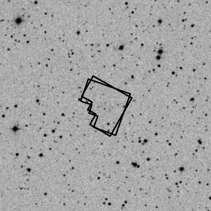
Figure 1.— The location of our WFPC2 fields overplotted on a digitized sky survey image of Andromeda V. The field is approximately 12 arcmin a side; North is up and east is to the left.

Figure 2.— The color-magnitude diagram of And V derived from archival HST/WFPC2 imaging.

Figure 3.— The color-magnitude diagram of And V showing the locations of the 10 high confidence RR Lyrae variables (filled circles). The open triangles are the simulated field stars created using the Besancon Galaxy model of Robin et al. (2003).

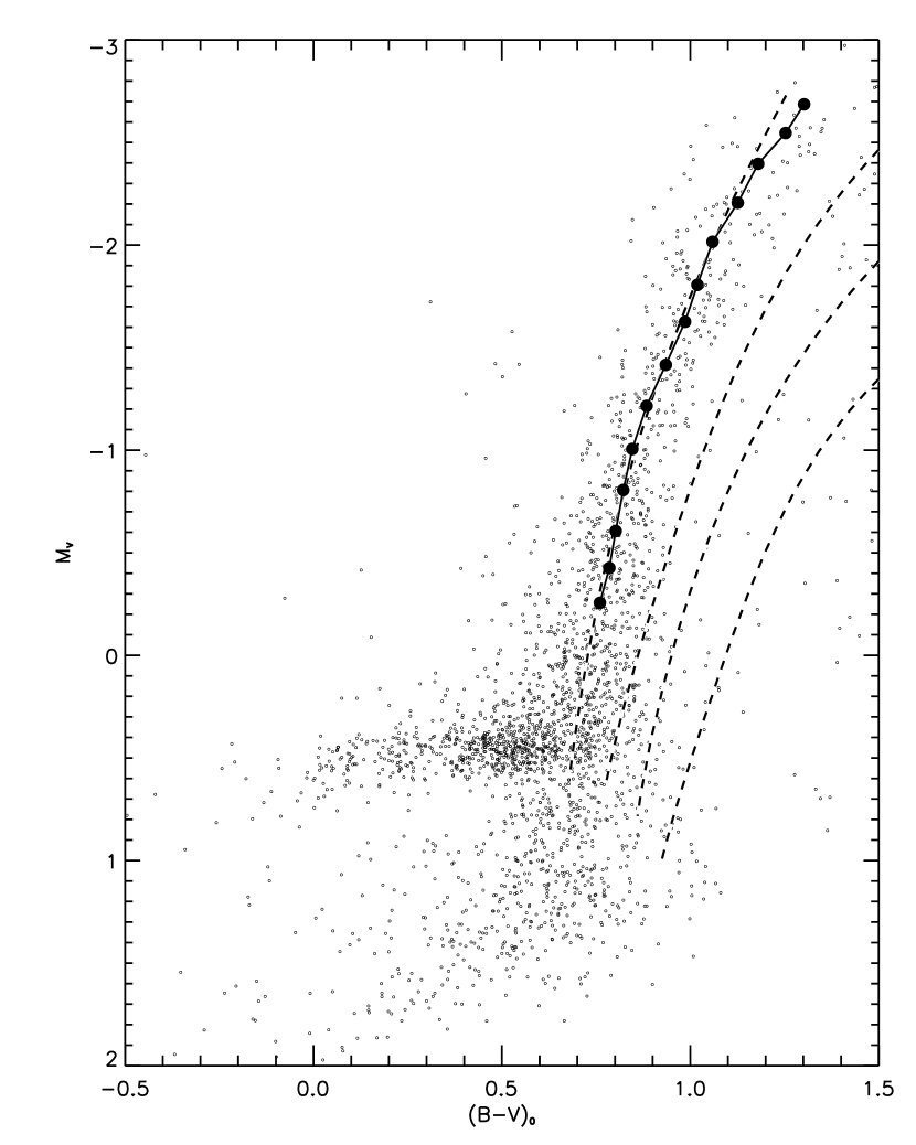
Figure 4.— The distance and reddening corrected CMD of And V along with our derived mean red giant branch sequence (filled circles connected by a solid line). Overplotted as dashed lines are the Galactic globular cluster fiducials of (left to right) M15, NGC 6752, NGC 1851, and 47 Tucanae from Sarajedini & Layden (1997) representing metallicities of –2.17, –1.54, –1.29, and –0.71, respectively, on the Zinn & West (1984) scale.

Figure 5.— The color histogram of red giant stars located in the range $23<V<24$. The color differences are measured relative to the mean RGB sequence illustrated in Fig. 4.

Figure 6.— The raw and folded light curves of high confidence variable 8. The upper left and upper right plots are the raw light curves for the two observing windows. The bottom plot contains the folded light curves and fitted templates.

References

- (1) Armandroff, T. E., Davies, J.E., Jacoby, G.H. 1998, AJ, 116, 2287
- (2) Burstein, D., & Heiles, C. 1982, AJ, 87, 1165
- (3) Caldwell, N., Armandroff, T.E., Da Costa, G.S., Seitzer, P. 1998, AJ, 115, 535
- (4) Caldwell, N. 1999, AJ, 118, 1230
- (5) Chaboyer, B. 1999, in Post-Hipparcos cosmic candles, edited by A. Heck and F. Caputo. (Dordrecht ; Boston) Astrophysics and space science library, Vol. 237), p.111
- (6) Charbonneau, P. 1995, ApJS, 101, 309
- (7) Da Costa, G.S., Armandroff, T.E., Caldwell, N., & Seitzer, P. 1996, AJ, 112, 2576
- (8) Da Costa, G.S., Armandroff, T.E., Caldwell, N., & Seitzer, P. 2000, AJ, 119, 705
- (9) Da Costa, G.S., Armandroff, T.E., & Caldwell, N. 2002, AJ, 124, 332
- (10) Davidge, T.J., Da Costa, G.S., Jørgensen, I., Allington-Smith, J.R. 2002, AJ, 124, 886
- (11) Dolphin, A. 2000, PASP, 112, 1383
- (12) Dotter A., Chaboyer, B., Jevremović, D., Baron, E., Ferguson, J., Sarajedini, A., & Anderson, J. 2007, AJ, 134, 376
- (13) Font, A. S., Johnston, K. V., Bullock, J. S., & Robertson, B. E. 2006, ApJ, 646, 886
- (14) Harbeck, D., Grebel, K., Holtzman, J., Guhathakurta, P., Brandner, W., Geisler, D., Sarajedini, A., Dolphin, A., Hurley-Keller, D., Mateo, M. 2001, AJ, 122, 3092
- (15) Lee, Y., Demarque, P., & Zinn, R. 1990, ApJ, 350, 155
- (16) Layden, A. C. 1995, AJ, 110, 2312
- (17) Layden, A.C. 1998, AJ, 115, 193
- (18) Liu, T. & Janes, K. A. 1990, ApJ, 354, 273
- (19) Martinez-Delgado, D., & Aparicio, A. 1997, ApJ, 480, L107
- (20) Martinez-Delgado, D., Aparicio, A., & Gallart, C. 1999, AJ, 118, 2229
- (21) McConnachie, A.W., Irwin, M.J., Ferguson, A.M.N., Ibata, R.A., Lewis, G.F., Tanvir, N., 2005, MNRAS, 356, 979
- (22) Mould, J. R., Kristian, J., & Da Costa, G. S. 1983, ApJ, 270, 471
- (23) Robin, A.C., Reylé, C., Derrière, Picaud, S. 2003, AA, 409, 523
- (24) Sandage, A. R. 1990, ApJ, 350, 603
- (25) Sandage, A. R. 1993, AJ, 106, 687
- (26) Sarajedini, A., Layden, A. 1997, AJ, 113, 264
- (27) Sarajedini, A., Barker, M., Geisler, D., Harding, P., Schommer, R. 2006, 132, 1361
- (28) Tinsley, B. M. 1978, ApJ, 222, 14
- (29) Zinn, R. J., & West, M. J. 1984, ApJS, 55, 45