Measurement of the decay of Fock states in a superconducting quantum circuit

Abstract

We demonstrate the controlled generation of Fock states with up to 15 photons in a microwave coplanar waveguide resonator coupled to a superconducting phase qubit. The subsequent decay of the Fock states, due to dissipation, is then monitored by varying the time delay between preparing the state and performing a number-state analysis. We find that the decay dynamics can be described by a master equation where the lifetime of the $n$-photon Fock state scales as $1/n$, in agreement with theory. We have also generated a coherent state in the microwave resonator, and monitored its decay process. We demonstrate that the coherent state maintains a Poisson distribution as it decays, with an average photon number that decreases with the same characteristic decay time as the one-photon Fock state.

Fock states are the eigenstates of the harmonic oscillator, and as such play a fundamental role in quantum communication and information. Due to the linear nature of the harmonic oscillator, transitions between adjacent Fock states are degenerate, making it impossible to generate and detect such states with classical linear techniques. Interposing a non-linear quantum system, such as that provided by a two-level qubit, allows such states to be probed unambiguously meek1996 ; cira1993 ; varc2000 ; bert2002 ; waks2006 ; guer2007 ; wall2004 ; hofh2008 ; joha2006 ; houc2007 ; sill2007 ; maje2007 ; schu2007 ; asta2007 ; fink2008 . However, the deterministic generation and characterization of Fock states with arbitrary photon numbers has not been demonstrated until recently hofh2008 , using a superconducting phase qubit coupled to a microwave resonator. The exquisite control provided by this implementation allows new tests of the fundamental physics of Fock states.

In this Letter, we present the first experimental measurement of the time decay of Fock states in a superconducting circuit. Although measurements of the relaxation dynamics have been done for the 2-phonon Fock state of a trapped ion coupled to a zero-temperature amplitude reservoir turc2000 , and proposed for higher $n$ Fock states of photons by performing a statistical analysis of a sequence of quantum non-demolition measurements guer2007 , a direct measurement beyond $n=2$ has not been attempted to date. The experiment described here is performed with a system similar to that in Ref. hofh2008 , but using a microwave resonator with significantly better performance, allowing the generation of Fock states with up to 15 photons. The subsequent decay of the Fock states, as well as the decay of a coherent state generated by a classical microwave pulse, have been directly measured and shown to display the expected dynamics. More importantly, we confirm that the lifetime of an $n$-photon Fock state accurately scales as $T_{n}=T_{1}/n$, where $T_{1}$ is the lifetime for the $n=1$ Fock state lu1989 . The lifetime $T_{n}$ scales as $1/n$ because each of the $n$ photons can independently decay.

In our experiment, the Fock states are generated by first driving the phase qubit from the ground $\left|g\right\rangle$ to the excited $\left|e\right\rangle$ state, during which the qubit and resonator are tuned out of resonance. We then turn on the coupling between the qubit and resonator by frequency-tuning them into resonance, allowing the qubit to transfer the photon to the resonator, generating an $n=1$ photon Fock state in the resonator and leaving the qubit in its $|g\rangle$ state. The qubit is then de-tuned from the resonator, so that the subsequent photon dynamics are determined by the resonator parameters alone. Because this sequence can be repeated $n$ times to produce an $n$-photon Fock state, this method is scalable to arbitrary photon numbers, limited only by the resonator decoherence time, the photon transfer speed through the qubit-resonator coupling, and the fidelities of the qubit $\left|e\right\rangle$ state preparation and the qubit-resonator tuning pulse. A resonator with a relatively long $T_{1}$ is thus desirable for both preparing high $n$ Fock states and measuring the subsequent decay dynamics.

Our device is composed of a half-wavelength coplanar waveguide resonator, capacitively coupled to a superconducting phase qubit, as shown in Fig. 1. It has a layout similar to that used in previous experiments neel20081 ; hofh2008 . In order to improve the resonator lifetime $T_{1}$, we have implemented a new design and fabrication procedure, that reduces the amount of amorphous dielectric in the vicinity of the resonator, thereby reducing microwave dielectric loss ocon2008 . We also used a resonator fabricated from superconducting Re (with $T_{c}\approx 1.8$ K), as this metal has substantially less native oxide than Al, which was used previously. As depicted in Fig. 1, the fabrication incorporates two resonator designs on the same wafer, allowing us to measure the resonator quality factor $Q$ from a classical resonance measurement ocon2008 , as well as the resonator $T_{1}$ using a qubit-based measurement hofh2008 . The layout of the two resonator designs are as identical as possible, to match any dissipation due to (unwanted) radiating modes in the microwave circuit.

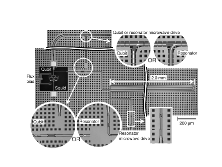
Figure 1: Photomicrograph of a coplanar waveguide resonator coupled to a phase qubit. The total length of the half-wavelength resonator is 8.8 mm. The insets show the two designs of the microwave lines that were varied in fabrication to connect the resonator either to a qubit or a classical preamplifier, allowing qubit-based $T_{1}$ or classical resonator $Q$ measurements, respectively.

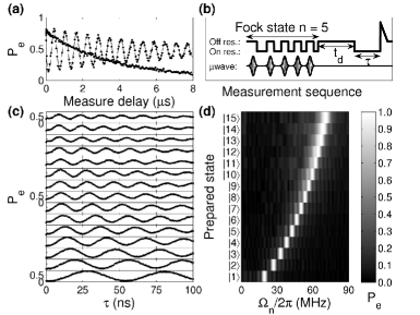
Figure 2: (a) Measurements of energy decay and Ramsey fringes for the resonator. Lines are fits to the data, yielding a resonator $T_{1}^{\prime}=3.47\ \mu\textrm{s}$ and $T_{2}^{\prime}=6.53\ \mu\textrm{s}$. (b) Pulse sequence used for the experiment, showing both the flux bias (top) and microwaves (bottom) needed to generate the $n=5$ Fock state. (c) Experimental data showing the state probability $P_{e}$ for the excited state $\left|e\right\rangle$ versus the qubit-resonator interaction time $\tau$ during a Fock state readout (see text). The decrease in the qubit oscillation period from bottom to top, scaling as $\sqrt{n}$, is expected from the Jaynes-Cummings model for an $n$-photon Fock state. For each panel, the y-axis ranges from 0% to 85%. The purity of the sinusoidal oscillations indicates the high fidelity of the state preparation. (d) Fourier transform of the data in (c). For each Fock state, the Fourier amplitude (gray scale) is normalized to the maximum peak amplitude.

The qubit is characterized using pulse sequences described previously luce2008 . We found an energy relaxation time $\approx 600\,\textrm{ns}$, a phase coherence time $\approx 100\,\textrm{ns}$, and a measurement visibility between the qubit $\left|g\right\rangle$ and $\left|e\right\rangle$ states of close to 90%. The initial characterization of the microwave resonator was made using a pulse sequence that swaps a photon into and out of the resonator, as described above and in Ref. neel2008 . The decay of the resonator state measured in this manner is plotted in Fig. 2(a), showing a decay time $T_{1}^{\prime}=3.47\ \mu\textrm{s}$ that is three times longer than in our previous experiment hofh2008 . The decay time for a Ramsey sequence gives $T_{2}^{\prime}=6.53\ \mu\textrm{s}$, approximately twice the resonator $T_{1}^{\prime}$, which indicates a long intrinsic dephasing time for the resonator, $T_{\phi}^{\prime}\gg T_{1}^{\prime}$, as expected. In addition, the classical measurement ocon2008 of the resonator quality factor $Q\approx 130,000$ at low power predicts $T_{1}=Q/\omega_{r}=3.15\ \mu\textrm{s}$, consistent with the qubit $T_{1}$ measurement. Here, $\omega_{r}/2\pi=6.570\ \textrm{GHz}$ is the resonator oscillation frequency, in agreement with design calculations that include the kinetic inductance of the Re center conductor. A spectroscopy measurement hofh2008 yields a splitting size of $\Omega/2\pi=19.0\pm 0.5\ \textrm{MHz}$, as expected for the qubit-resonator coupling strength due to a design value of coupling capacitor of $2.6\ \textrm{fF}$. The qubit-resonator coupling can be turned off by tuning the qubit off-resonance. In this experiment the detuning was $400\ \textrm{MHz}$.

The pulse sequence for generating and measuring Fock states hofh2008 is illustrated in Fig. 2(b). The timing of the pulses is based on the Jaynes-Cummings model jayn1963 , which predicts that on resonance, the occupation of the two coupled degenerate states $\left|g,n\right\rangle$ and $\left|e,n-1\right\rangle$, with $n$ and $n-1$ photons in the resonator, respectively, will oscillate with a radial frequency $\Omega_{n}=\sqrt{n}\Omega$. For generation, the $n^{\rm{th}}$ photon is loaded from the excited state of the qubit using a carefully controlled interaction time of $\pi/\Omega_{n}=\pi/\sqrt{n}\Omega$. The subsequent readout of the resonator state is performed by tuning the qubit, initially in its ground state, into resonance with the resonator, and measuring the subsequent evolution of the qubit excited state probability $P_{e}$ as a function of the interaction time $\tau$. A Fourier transform (FT) of $P_{e}(\tau)$ gives the occupation probability of the $n$-photon Fock state as the Fourier component (in amplitude) of $P_{e}$ at the frequency $\Omega_{n}$.

Figure 2(c) shows $P_{e}$ versus interaction time for a number of different Fock states. For these data, the readout starts after a delay time $t_{d}=150\,\textrm{ns}$. For an interaction time $\tau$ from 0 to 300 ns, sinusoidal oscillations are clearly visible for Fock states from $n=1$ up to $n$ = 15. The visibility of the $n=1$ sinusoidal oscillation is about 75%, which results from the high fidelity of the state preparation and the high visibility of qubit readout close to 90%. The frequency increases with increasing $n$, consistent with the predicted $\sqrt{n}$ dependence. A FT of the data is shown in Fig. 2(d), indicating the spectral purity of the oscillations. The Fock state $n=1$ gives a Rabi frequency of 19.33 MHz, consistent with the splitting obtained from spectroscopy.

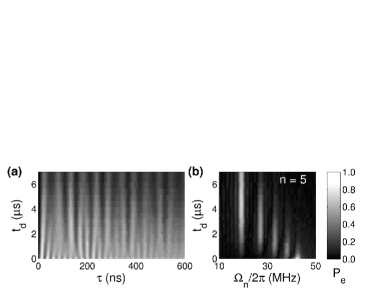
Figure 3: (a) Qubit $\left|e\right\rangle$ state probability $P_{e}$ (gray scale) as a function of the qubit-resonator interaction time $\tau$ (horizontal axis) and the measure delay $t_{d}$ (vertical axis). (b) Fourier transform (along horizontal axis) of data in (a), showing decay of the Fock states with increasing time. The Fourier spectrum is normalized to the maximum peak amplitude corresponding to $n=5$ at $t_{d}=0$.

The decay dynamics of the Fock states can be probed by varying the measurement delay $t_{d}$ in the pulse sequence. An example is shown in Fig. 3(a), where $P_{e}$ is plotted in gray scale versus $t_{d}$ and $\tau$ for the Fock state $n=5$. At $t_{d}=0$, a periodic oscillation of $P_{e}$ is observed that corresponds to the occupation of the $n=5$ Fock state. With increasing $t_{d}$, the oscillation evolves into a complex aperiodic pattern, finally changing to a slower oscillation frequency for $t_{d}\approx 7~{}\mu\textrm{s}$. The corresponding FT analysis is shown in Fig. 3(b). The system starts in the Fock state $n=5$, and then evolves to a mixed state with several frequencies present in the spectrum, and eventually decays to a mixture of the Fock states $n=1$ and $n=0$.

As no phase information is involved, the decay of Fock states can be simply described by changes in the state probabilities. The master equation is given by

$$\frac{dP_{n}(t)}{dt}=-\frac{P_{n}(t)}{T_{n}}+\frac{P_{n+1}(t)}{T_{n+1}},$$ (1)

where $P_{n}(t)$ and $T_{n}$ are the occupation probability and the decay time of the $n$-photon Fock state, respectively. To compare our data with theory, we plot in Fig. 4(e) the normalized amplitude in the FT as a function of the measure delay $t_{d}$ for each Fock state in the spectrum of Fig. 3(b). Also shown in Fig. 4 is the decay of Fock states from $n$ = 1 (a) to $n$ = 6 (f), similarly obtained from the FT spectrum. The predictions from the master equation (lines) fit the data remarkably well for Fock states up to $n=6$, taking as initial conditions the measured state probabilities. The fitting parameters for $T_{n}$ for each panel are listed in Table 1. The average values show good scaling with the predicted $T_{n}\approx T_{1}/n$ for $n=1$ to 5. Since 600 ns-long time traces are used for the FT analysis to retrieve the Fock state probability, it is reasonable to begin to see some deviation from the prediction for $T_{6}\approx 640\ \textrm{ns}$.

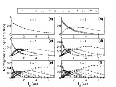
Figure 4: Time decay of Fock states from $n$ = 1 (a) to $n$ = 6 (f), taken from the amplitude of the FT data. Occupation probabilities of the Fock states, $P_{n}$, are plotted with symbols defined at top panel. Data are normalized by choosing the total occupation probability, including $n=0$, at the measure delay $t_{d}=0$ to be unity hofh2008 . Lines are fits to the data; the $n$-state lifetimes $T_{n}$ as extracted from the fits are listed in Table 1.

Table 1: Lifetimes (in units of $\mu\textrm{s}$) of the $n$-photon Fock states taken from fits to Fig. 4(a)-(f), respectively. The averages are listed in the second-to-last row, along with the expected $T_{1}/n$ scaled from the measurement of $T_{1}=3.20\ \mu\textrm{s}$. The values in parentheses are not included in the averages, as the fits are only reliable if there is a sizeable exponential decay of the data at times less than 7 $\mu\textrm{s}$, a limit set by our electronics.

n	$T_{1}$	$T_{2}$	$T_{3}$	$T_{4}$	$T_{5}$	$T_{6}$
1	2.96
2	3.21	1.65
3	3.44	1.58	1.01
4	(4.15)	1.60	1.02	0.81
5	(6.29)	(1.88)	1.11	0.79	0.65
6	(5.49)	(1.78)	1.08	0.77	0.66	0.64
Avg.	3.20	1.61	1.06	0.79	0.66	0.64
$T_{1}/n$	3.20	1.60	1.07	0.80	0.64	0.53

The FT analysis can also be used to test the decay dynamics of a coherent state. A coherent state is a superposition of Fock states, with the occupation probability $P_{n}$ of the Fock state $n$ given by a Poisson distribution,

$$P_{n}(a)=\frac{a^{n}e^{-a}}{n!},$$ (2)

where $a$ is the average photon number. The resonator is first driven with a 100 ns classical microwave pulse, creating a coherent state with $a$ proportional to the drive pulse amplitude hofh2008 . After a measure delay $t_{d}$, the resonator state is read out using the qubit, initially in its ground state, in the same manner as discussed above. For a coherent state with $\langle n\rangle=a\approx 7.14$, the occupation probabilities of the Fock states versus the photon number $n$ are plotted in Fig. 5(a) for several time delays. At each delay time $t_{d}$, the Fock state probabilities (points) can be well described by the Poisson distribution given by Eq. 2 (lines), with $a$ as the fitting parameter. In Fig. 5(b), we plot $a$ as a function of $t_{d}$ obtained for the complete data set. The average photon number $a$ decays with a dependence that is fit by an exponential with a decay time $3.43~{}\mu\textrm{s}$, in good agreement with the measured resonator $T_{1}$.

We note that although the occupation probabilities of the Fock states still follow a Poisson distribution during the entire decay process, our analysis cannot distinguish a statistical mixture from a pure coherent state. A complete tomographic measurement is necessary in order to verify the phase coherence of the coherent state.

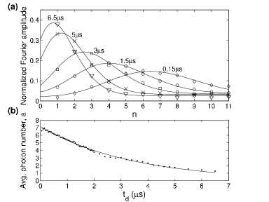
Figure 5: (a) Occupation probabilities for coherent state analysis, taken from the normalized Fourier amplitude versus Fock state number $n$ at a few example delay times. Data are normalized by choosing the total occupation probability at the measure delay $t_{d}=0$ to be unity, assuming that the $n=0$ probability at $t_{d}=0$ is negligible. Lines are fits to the data according to the Poisson distribution. (b) Average photon number $a$ versus the measure delay $t_{d}$, obtained from fits to data as shown in (a). The line is an exponential fit yielding a lifetime of $3.43\ \mu\textrm{s}$.

In conclusion, we have improved the decay time of our earlier resonator design by a factor of 3, and thereby generated high-fidelity Fock states with up to 15 photons. The time decay of both Fock and coherent states were directly measured, and shown to be in excellent agreement with the theoretical prediction of a master equation with $T_{n}=T_{1}/n$.

Acknowledgements. Devices were made at the UCSB Nanofabrication Facility, a part of the NSF-funded National Nanotechnology Infrastructure Network. This work was supported by IARPA under grant W911NF-04-1-0204 and by the NSF under grant CCF-0507227.

References

- (1) D. M. Meekhof, C. Monroe, B. E. King, W. M. Itano, and D. J. Wineland, Phys. Rev. Lett. 76, 1796 (1996).
- (2) J. I. Cirac, R. Blatt, A. S. Parkins, and P. Zoller, Phys. Rev. Lett. 70, 762 (1993).
- (3) B. T. H. Varcoe, S. Brattke, M. Weidinger, and H. Walther, Nature 403, 743 (2000).
- (4) P. Bertet et al., Phys. Rev. Lett. 88, 143601 (2002).
- (5) E. Waks, E. Dimanti, and Y. Yamamoto, N. J. Phys. 8, 4 (2006).
- (6) C. Guerlin et al., Nature 448, 889 (2007).
- (7) M. Hofheinz et al., Nature 454, 310 (2008).
- (8) A. Wallraff et al., Nature 431, 162 (2004).
- (9) J. Johansson et al., Phys. Rev. Lett. 96, 127006 (2006).
- (10) A. Houck et al., Nature 449, 328 (2007).
- (11) M. A. Sillanp, J. I. Park, and R. W. Simmonds, Nature 449, 438 (2007).
- (12) J. Majer et al., Nature 449, 443 (2007).
- (13) D. I. Schuster et al., Nature 445, 515 (2007).
- (14) O. Astafiev et al., Nature 449, 588 (2007).
- (15) J. M. Fink et al., Nature 454, 315 (2008).
- (16) Q. A. Turchette et al., Phys. Rev. A 62, 053807 (2000).
- (17) N. Lu, Phys. Rev. A 40, 1707, (1989).
- (18) M. Neeley et al., Phys. Rev. B 77, 180508(R), (2008).
- (19) A. D. O’Connell et al., Appl. Phys. Lett. 92, 112903 (2008).
- (20) E. Lucero et al., Phys. Rev. Lett. 100, 247001 (2008).
- (21) M. Neeley et al., Nature Physics 4, 523-526 (2008).
- (22) E. Jaynes and F. Cummings, Proc. IEEE 51, 89 (1963).